在晶片多處理器系統下以減少快取衝突為目的之動態工作排程方法

全文

(1)國立交通大學資訊科學與工程研究所碩士論文. 在晶片多處理器系統下以減少快取衝突為目的之動態工作排程方法 A Dynamic Task Scheduling Method for Less Cache Contention on Chip Multiprocessor Systems. 研究生：廖哲瑩指導教授：陳. 中華民國. 正. 教授. 九十五. 年六月.

(2) 在晶片多處理器系統下以減少快取衝突為目的之動態工作排程方法 A Dynamic Task Scheduling Method for Less Cache Contention on Chip Multiprocessor Systems. 研究生: 廖哲瑩. Student: Che-yin Liao. 指導教授: 陳. Advisor: Cheng Chen. 正. 國立交通大學資訊科學與工程研究所碩士論文. A Thesis Submitted to Institute of Computer Science and Engineering College of Computer Science National Chiao Tung University in partial Fulfillment of the Requirements for the Degree of Master in. Computer Science June 2006 Hsinchu, Taiwan, Republic of China. 中華民國九十五年六月.

(3) 在晶片多處理器系統下以減少快取衝突為目的之動態工作排程方法研究生: 廖哲瑩. 指導教授: 陳正教授. 國立交通大學資訊科學與工程研究所碩士班. 摘要積體電路製程的進步使得需要大量電晶體來實作的微處理器設計得以被付諸實行，晶片多處理器 (chip multiprocessor) 是這些新世代設計的其中一員。一個晶片多處理器有多個處理器核心，在晶片多處理器上的 L2 快取記憶體會由這些處理器核心共用，因此處理器核心間可能會發生快取衝突。快取衝突會為晶片多處理器的效能帶來負面影響，為了減少快取衝突我們提出了一個稱為 Hint-aided Cache Contention Avoidance (HCCA) 的動態工作排程方法。 HCCA 首先預測工作執行時可能使用的快取記憶體區段，並將會使用到相同快取記憶體區段的工作分開排程以減低快取衝突。在 HCCA 中包含三個階段，第一階段我們會由工作的程式碼中萃取出可以協助排班的資訊。接著，在第二階段我們會利用在第一階段萃取得來的資訊做出快取記憶體使用區段的預測。我們的預測是基於工作的程式碼所萃取得來的資訊，而工作的程式碼將會直接影響工作存取快取記憶體的模式，因此我們預期所做出的預測可以比其他的方法有較好準確率。最後，在第三階段我們根據於前一階段所做出的快取記憶體使用區段的預測結果做出工作排班。我們以模擬的方式評估 HCCA 的效能，模擬結果顯示 HCCA 可以使得晶片多處理器系統有較低的快取誤失率，並藉此可以改善整體效能。. i.

(4) A Dynamic Task Scheduling Method for Less Cache Contention on Chip Multiprocessor Systems Student: Che-yin Liao. Advisor: Prof. Cheng Chen. Institute of Computer Science and Engineering Nation Chiao Tung University. Abstract The chip multiprocessor is an emerging microprocessor architecture which attempts to utilize the integration increased by the advances of integrated circuit technologies. A chip multiprocessor contains multiple execution cores which share the on-chip L2 cache. Therefore, the cache contentions may occur among cores. In order to reduce cache contentions which cause negative impacts on performance, we propose a task scheduling technique named Hint-aided Cache Contention Avoidance (HCCA). HCCA attempts to avoid cache contentions by separately scheduling tasks predicted to use the same cache sets. HCCA contains three phases. The first phase analyzes binary images and extracts information used to support the predictions of cache set usages. Then, the second phase makes the cache set usage predictions according to the information extracts by the previous phase. The predictions are made according to the information extracted from binary images which directly affect how tasks accessing cache sets. Therefore, the predictions are expected to be more accurate than those made by previous methods. Finally, the scheduling decisions are made in the third phase according to the cache set usages predictions made in previous phase. We have constructed a simulator to evaluate the performance of HCCA. The simulation results show that HCCA has lower L2 cache miss rate than that of others and also have some improvement on overall IPC compared with other methods. ii.

(5) Acknowledgments I would like to express my sincere thanks to my advisor, Prof. Cheng Chen, for his supervision and advice. Without his guidance and encouragement, I could not finish this thesis. I also thank Prof. Jyj-Jiun Shann and Prof. Kuan-Chou Lai for their valuable suggestions. There are many others whom I wish to thank. I thanks to Yi-Hsuan Lee for her kindly advice suggestion. Ming-Hsien Tsai is delightful follow, I felt happy and relaxed because of your presence. Finally, I am grateful to my dearest family for their encouragement. 另外我也必須感謝 Auron Wu 在英文寫作方面的幫忙，沒有 Auron Wu 的大力協助我沒有辦法完成這份論文。. iii.

(6) Table of Contents 摘要.................................................................................................................................i Abstract...........................................................................................................................ii Acknowledgments.........................................................................................................iii Table of Contents...........................................................................................................iv List of Figures................................................................................................................vi Chapter 1 Introduction....................................................................................................1 Chapter 2 System Model and Related Work..................................................................5 2.1 System model.................................................................................................5 2.2 Related work...................................................................................................7 2.2.1 Cache partitioning approach...............................................................7 2.2.1.1 Dynamic cache partitioning for CMP/SMT systems..............7 2.2.1.2 Fair cache sharing and partitioning for CMP.........................8 2.2.2 Operating system scheduling approach..............................................9 2.2.2.1 Active-set supported task scheduling...................................10 2.2.2.2 Inter-thread cache contention prediction..............................10 2.2.2.3 Throughput-oriented scheduling..........................................12 Chapter 3 Hint-aided Cache Contention Avoidance Technique...................................14 3.1 Preliminary...................................................................................................14 3.2 Overview......................................................................................................15 3.3 Hint generation.............................................................................................17 3.3.1 Binary image dissection....................................................................18 3.3.2 Heap usage profiling.........................................................................19 3.4 Hint evaluation.............................................................................................22 3.5 Task scheduling............................................................................................29 Chapter 4 Preliminary Performance. Evaluation.....................................................35. 4.1 Simulation overview.....................................................................................35 4.2 Evaluation results.........................................................................................40 4.2.1 Prediction accuracy...........................................................................40 4.2.2 L2 miss rate.......................................................................................41 iv.

(7) 4.2.3 Overall performance.........................................................................45 Chapter 5 Conclusions and Future Work......................................................................47 5.1 Conclusions..................................................................................................47 5.2 Future work..................................................................................................48 Bibliography.................................................................................................................51. v.

(8) List of Figures Figure 2.1 A schematic view of a chip multiprocessor.....................................................5 Figure 2.2 The queuing diagram representation of task scheduling..................................6 Figure 2.3 Illustration of how interleaving accesses from another task determines whether the access will be a cache hit or cache miss, assuming a 4-way full associative cache............................................................................................11 Figure 3.1 Typical memory space layout of single task..................................................14 Figure 3.2 Overall flow of HCCA method......................................................................15 Figure 3.3 The high level programming language processing flow................................17 Figure 3.4 An example of sibling-child binary tree representation of basic blocks........18 Figure 3.5 The algorithm of the heap usage profiling.....................................................22 Figure 3.6 An example of Hint........................................................................................23 Figure 3.7 An example of the expected execution time adjustment of basic blocks.......26 Figure 3.8 The algorithm of the hint evaluation phase....................................................27 Figure 3.9 The algorithm of the hint evaluation phase. (cont.).......................................28 Figure 3.10 An example of the first stage of gang grouping...........................................31 Figure 3.11 An example of the second stage of gang grouping......................................32 Figure 3.12 The algorithm of the task scheduling phase.................................................33 Figure 4.1 The trace generator and the hint generator.....................................................35 Figure 4.2 The architecture of our simulator...................................................................36 Figure 4.3 The configuration of memory simulator........................................................37 Figure 4.4 The list of tasks used in our simulation..........................................................38 Figure 4.5 The sorted task list.........................................................................................39 Figure 4.6 The simulation workloads..............................................................................39 Figure 4.7 The prediction accuracy.................................................................................41 Figure 4.8 The simulation result of workload 1..............................................................42 Figure 4.9 The simulation result of workload 2..............................................................42 Figure 4.10 The simulation result of workload 3............................................................43 Figure 4.11 Overall IPC under various workloads for different cache associativity......44. vi.

(9) Figure 4.12 The improved percentage of IPC over Round-Robin under various associativity...................................................................................................45. vii.

(10)

(11) Chapter 1 Introduction The advances in integrated circuit processing technologies increase the transistor density and allow more micro-processor design options[1 -3]. The chip 2. multiprocessing (CMP) architecture is one of the micro-processor designs that attempt to utilize the increased integration[4, 5]. In a typical chip multiprocessor, it consists a set of identical cores, and each core has its own execution resources such as ALU, FPU, L1 caches, register file and control logics. The L2 cache and its lower memory hierarchy are shared by these cores[6 -8]. By taking advantage of the thread 7. level parallelism, chip multiprocessors can achieve better performance per watt scalability with advances of integrated circuit technologies than single core processors. This makes chip multiprocessors a promising microprocessor design for emerging high-performance and power-efficiency computing. Besides, sharing the L2 cache allows high cache utilization and avoids duplicating the cache hardware resources. However, cache sharing may cause cache contentions among executed tasks[9]. Because the L2 cache is sharing among all executed tasks, the data block loaded by one task may be replaced by the data block loaded by another task. The task which loses its data block from cache will experience a cache miss if it accesses the evicted data again. However, this cache miss would not occur in a single core processor environment. This extra L2 miss called cache contention, which will cause the processor to fetch data from the lower memory hierarchy. Fetching data from the lower memory hierarchy usually takes more time than directly fetching from the higher memory hierarchy, hence it lengthens the task execution time[10 1112. 13]. Therefore, cache contentions may harm the performance of chip multiprocessor -1-.

(12) systems by causing extra L2 cache misses and lengthening the execution time of tasks. In order to reduce cache misses caused by cache contentions, many techniques have been proposed in recent years[10 -12, 14, 15]. We classify these proposed 11. techniques into two categories: one is cache partitioning[10, 11] and the other is operating system scheduling[12, 14, 15]. The key idea of cache partitioning approach is to partition cache blocks into groups. Then, each group is allocated to an executed task. During executing, the number of blocks in a group may be changed to fit the cache need of tasks. Cache contentions can be completely avoided if all groups are disjoint. However, groups may be overlapped to increase the flexibility. The operating system scheduling approach attempts to avoid cache contentions by separately scheduling tasks which may use the same cache sets. A mechanism to predict the cache set usage is required for the operating system scheduling approach because the task scheduling decisions have to be made before the tasks actually executing on the cores. For cache partitioning approach, tasks may still suffer from cache contentions if all concurrently executed tasks frequently access memory and cause big overlap among groups. However, the operating system scheduling approach can resolve this by separately scheduling the tasks which are predicted to use the same cache sets. In this thesis, we propose an effective task scheduling method, called Hintaided Cache Contention Avoidance (HCCA) to reduce the number of cache contentions for chip multiprocessor systems. HCCA contains the following three phases: hint generation, hint evaluation and task scheduling. Like previous methods, HCCA first predict the cache set usage. Then, it attempts to minimize the cache. -2-.

(13) contentions among concurrently executed tasks by separately scheduling tasks using the same cache sets. In previous task scheduling methods, they usually predict the cache set usage of tasks according to their previous usage. However, because cache set usages may change during the execution of tasks, making predictions according to the previous cache set usage may not be able to predict these changes. Instead of using the previous cache set usage, we make cache set usage predictions according to the information extracted from the corresponding binary images of tasks. The binary image contains an ordered set of machine instruction codes which instructs the processor to accomplish the task. Therefore, it directly affects the behavior of a task. However, analysis the binary image needs unacceptable long time for the task scheduling. We resolve this by first generating an abstract of a binary image which we call it a hint before running the task. This phase is called hint generation. While executing the tasks, we make the cache set usage prediction according the hint. We call this phase hint evaluation. Then, we make the scheduling decision according to the cache set usage predictions. This phase is called task scheduling. In summary, HCCA contains the following three phases. The hint generation phase generates hints from binary images. The hint evaluation phase makes the cache set usage predictions according the hints. The task scheduling phase make the scheduling decisions according to the predicted cache set usages. For evaluating the performance, we construct a simulator and compare our method with previous work. We form workloads with benchmark programs and input data sets from SPEC 2000[16]. Then these workloads are used to test the scheduling mechanisms. From the simulation results, we can see that HCCA has. -3-.

(14) lower L2 cache miss rate than that of others and also have some improvement on overall IPC (instruction per cycle) compared with other methods. This thesis is organized as follows. Chapter 2 introduces the system model and reviews some related work. Chapter 3 describes our HCCA technique in some detail. Performance evaluations are presented in Chapter 4. Finally, conclusions and future work are given in Chapter 5.. -4-.

(15) Chapter 2 System Model and Related Work In this chapter, we will first introduce our system architecture and some terminologies in section 2.1. Then, we will briefly survey some related work in section 2.2.. 2.1 System model We make several assumptions for our chip multiprocessor system. First, we assume that our chip multiprocessor system consists a m cores chip multiprocessor, as shown in Figure 2.1. Each core has its own hardware context, such as register file and L1 caches. Every processor core shares the unified L2 cache with the other cores[6]. We assume that the L2 cache in processor package is a n-way set associative cache. An example of chip multiprocessor is the IBM POWER4 which contains two cores. The cores in POWER4 share an 8-way unified L2 cache[8]. Second, we assume the operating system used in our chip multiprocessor system provides necessary communication and synchronization mechanisms for executed tasks. A task is a unit of atomic work which is not parallelizable. Parallelized tasks. core 0 core 1. shared L2 cache. core m-1 processor package. Figure 2.1 A schematic view of a chip multiprocessor. -5-. off-chip memory.

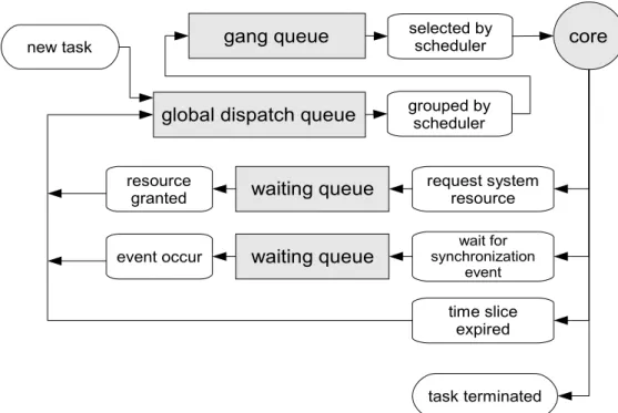
(16) gang queue. new task. global dispatch queue. selected by scheduler. core. grouped by scheduler. resource granted. waiting queue. request system resource. event occur. waiting queue. wait for synchronization event. time slice expired. task terminated. Figure 2.2 The queuing diagram representation of task scheduling.. can be implemented as several sequential tasks and maintain dependency with synchronization mechanisms provided by operating system[17, 18]. There is a task scheduler in system, which chooses tasks for cores to execute. As shown in Figure 2.2, the task scheduler maintains a global dispatch queue and a gang queue. When a task comes to system, it is first placed into the global dispatch queue. Then, tasks will be grouped into small groups called gangs. The number of tasks in a gang is equal to the number of cores in system. Tasks in the same gang will be concurrently scheduled on cores. We also call a set of tasks simultaneously executed on the cores as “co-scheduled tasks” or “task mix”. When the gang is scheduled, tasks in it will be assigned a short time interval called time slice. The task leaves core when it is terminated, the allocated time slice is expired, or it is going to wait for some system resource [18, 19]. If one of the executing task leaves core before its time slice expires, other tasks will be forced to give up the remaining time. -6-.

(17) slice and leave cores. When the scheduler is activated, it will first check the gang queue to see if there exists any unscheduled gang. Otherwise, tasks in the global dispatch queue will be grouped into gangs and push into the gang queue for future scheduling. We assume that the task scheduler is executed on a dedicated system processor. The m cores chip multiprocessor executes dispatched tasks in parallel with the scheduler. Hence the scheduling overhead does not cause uncertainty in the executions of the dispatched tasks [14, 15].. 2.2 Related work We classify the approaches for less cache contention on chip multi-processor architecture into two categories: one is cache partitioning and the other is operating system scheduling. These approaches will be described in the following sections.. 2.2.1. Cache partitioning approach The cache partitioning approach attempts to partition cache blocks into groups.. Each group is allocated to an executed task. The number of blocks in a group will be adjusted to fit the cache demand of tasks during executing. Cache contentions can be completely avoided if all groups are disjoint. However, groups may overlap to increase the flexibility. We briefly survey two methods in the following. 2.2.1.1. Dynamic cache partitioning for CMP/SMT systems [10]. This technique uses an additional hardware to account numbers of cache hit and miss in a specified time period t. The cache partition is dynamically adjusted according to the accounting results. A task causes more cache misses will be. -7-.

(18) allocated more cache blocks to reduce the cache misses. A modified LRU cache replacement policy is proposed to realize the cache partitioning. Besides the number of cache hit and miss, the modified LRU replacement policy also need the number of cache blocks occupied by each task. The collected data is used to find out the over-allocated task. The over-allocated task is the task which the number of allocated cache blocks is more than the number of accessed blocks in a specified time period t. Considering the cache miss of task T, if T is an over-allocated task then the victim block is chosen within cache blocks occupied by task T with LRU policy. Otherwise, the victim block is chosen within cache blocks occupied by other over-allocated tasks. If there does not exist any over-allocated tasks, the standard LRU policy is used to select the victim block from all cache blocks. The drawback of this method is that it requires extra partitioning logic circuits. These extra circuits will increase the miss penalty. 2.2.1.2. Fair cache sharing and partitioning for CMP [11]. Kim et al. address the unfair cache sharing problem. The conventional operating system scheduler usually assumes the resource sharing uniformly impacts co-scheduled tasks. However, this assumption is often unmet on chip multiprocessor system, because the abilities of tasks to compete cache space are different. The ability of a task to compete cache space is determined by its temporal reuse behavior, which are usually different among tasks. If the cache block loaded by a task is being replaced by another task frequently, the task which lost cache block will suffer from higher cache miss rate due to the replacement. These extra cache misses will result in negative effect on the system throughput. In order to solve this -8-.

(19) problem, a metric to measure the fairness of cache sharing and a mechanism to adjust the cache sharing are proposed. Considering the task T, the proposed metric is shown as follows: shr. MISS T FairMetric T = MISS ded T. ......................................................................(2.1). In this formula, MISS shr T denotes the miss rate of task T when it shares the cache with other tasks, and MISS ded T denotes the miss rate of task T when it runs alone with dedicate cache. A task Ti with larger FairMetric(Ti) value indicates relative more cache contention which is caused by sharing cache with other tasks. In an ideal situation, all values would be the same. The same values indicate that the increased miss rate causes equal impacts for all tasks. This metric is used in cache sharing adjustment which is realized by modifying the cache replacement policy. When a cache miss occur, the metric is evaluated for each running task. The victim block is selected within those cache blocks allocated by the task whose value is the smallest. As the method proposed by Suh et al. [10], this method also need adding extra logic circuits to the circuits of cache which will increase the miss penalty. The performance of memory accesses may suffer by extra cache miss penalty.. 2.2.2. Operating system scheduling approach The operating system scheduler approach attempts to select co-scheduled tasks. which use different part of cache to minimize occurrences of cache contention. The scheduling decision must be made before tasks being executed, so the scheduler. -9-.

(20) requires to predict the memory behavior of tasks. We introduce three methods briefly in the following. 2.2.2.1. Active-set supported task scheduling [14]. T. Sherwood et al.[20] have shown that the task behavior is typically periodic and predictable, and so is the cache access behavior. Hence, [14] attempts to use this property to predict the cache access behavior. The future cache usage is predicted by the past cache usage. Then the tasks which might use different cache regions are coscheduled. Thus, it reduces the possibility of co-scheduled tasks using the same cache regions. Settle et al. propose a monitoring hardware to record the number of cache accesses for cache sets. The task scheduling decisions are made based on the recorded results. The cache set are considered as frequently access cache region if it has the number of accesses larger than a preset threshold. Tasks with different frequently access cache regions are simultaneously scheduled. This method assumes that the future memory behavior can be perfectly predicted by using past memory behavior. However, tasks may change its behavior during their execution, and so do their cache access patterns. The prediction policy may not be able to react these changes instantly. Therefore, the change of task behavior may result in false prediction and lead to an inferior scheduling decision. 2.2.2.2. Inter-thread cache contention prediction [12]. Chandra et al. propose a method called Prob to predict the number of cache contentions in a given task mix. Tasks running on a chip multiprocessor must share memory hierarchy. Therefore, memory accesses from co-scheduled tasks will be interleaved. Figure 2.3 shows two cases of interleaving accesses. Both cases. - 10 -.

(21) T1R: A B A T2R: U V V W case 1: A U B V V A W. case 2: A U B V V W A. Hit. Miss. Figure 2.3 Illustration of how interleaving accesses from another task determines whether the access will be a cache hit or cache miss, assuming a 4-way full associative cache.. interleave accesses from task T1 with task T2. The access trace of T1 is denoted by T1R, and the access trace of T2 is denoted by T2R. The uppercase letters in access trace denote the memory addresses. Assuming a 4-way full associative cache, the second access to A is a cache hit in case 1, but a cache miss in case 2. The difference is that case 2 interleaved more accesses which load new blocks into cache. These interleaved accesses make the data block which loaded by first access to A been evicted. Prob uses a probabilistic approach to predict miss rate of a task mix. It needs the cache access traces for all tasks in the task mix. All possible interleaved access traces are exhaustively listed. The probability of an individual cache hit which becomes a cache miss is computed. Then, by multiplying the number of cache hits in access traces and the computed possibility, we can get the expect value of overall miss rate. The prediction can be used as one of the scheduling criteria of task scheduler to reduce the cache contentions. The disadvantage of Prob is that it exhaustively evaluates all possible interleaved access traces. This evaluation would be very expansive while the number of tasks increases.. - 11 -.

(22) 2.2.2.3. Throughput-oriented scheduling [15]. Fedorova et al. propose a modified balance-set[21] scheduling algorithm to decrease the shared L2 cache miss on chip multi-threading system. It first estimates miss rate of all possible task mixes by adapting the StatCache[22] probabilistic model. The StatCache model used in this approach is developed by Berg and Hagersten. It is used to predict the miss rate of single task with previously recorded reuse distance information[23]. Fedorova et al. proposed a merging method called AVG to combine individual miss rate predictions into the miss rate prediction of coscheduled tasks. AVG adjusts StatCache by assuming the numbers of cache blocks accessed by all tasks are equal. The overall miss rate for co-scheduled tasks is the average miss rate of all tasks. After predicting the miss rate of task mix, tasks are divided into groups according to the estimated results. Then, Fedorova et al. use a mechanism integrated with balance-set[21] and StatCache[22] to schedule tasks. When the scheduling decision is made, it first generates all possible task mixes from the global dispatch queue. Second, it predicts miss rate for all possible task mixes with StatCache and AVG. Then, task mixes with predicted miss rates lower than a given threshold are considered to schedule. Final scheduling decision is made with other scheduling factors, such as priority and waited time. The drawback of this approach is that the AVG mechanism simply assumes all tasks allocated equal fraction of cache. However, this assumption is not always true, since the abilities of tasks to compete cache space are different, as discussed in [11]. This might result in inaccurate prediction in set-associative cache, and lead to suboptimal scheduling.. - 12 -.

(23) From the related work, the cache partitioning approaches focus on partitioning cache for co-scheduled tasks. However, if all of the co-scheduled tasks frequently access cache then these tasks may still suffer by cache contentions. The operating system approaches can resolve this by selecting co-scheduled tasks which use the different part of the cache. In other words, the cache hardware only affects activities on the scale of tens to thousands of cycles. On the other hands, the operating system controls the resources and activities at the larger time scale, million of cycles. We have more opportunities to improve the system behavior through the operating system. Besides, the operating system task scheduler is usually implemented as software. By using software mechanisms, it is possible to build systems that can evolve when new techniques to be discovered. Furthermore, software approaches allow us to do some workload specific tuning. These benefits form our basis to select the operating system task scheduling approach. In next chapter, we will describe the basic concepts and principles of our method in some detailed.. - 13 -.

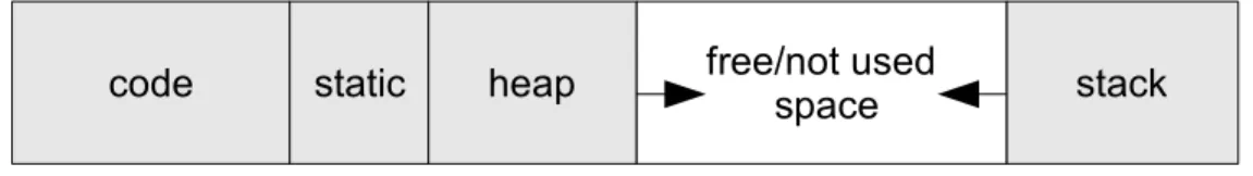
(24) Chapter 3 Hint-aided Cache Contention Avoidance Technique In this chapter, we will first define some terminologies in section 3.1 and give the overview of our method in section 3.2. The analysis mechanism is described in section 3.3. The final prediction and scheduling mechanisms are described in section 3.4 and 3.5.. 3.1 Preliminary First, we introduce the memory space layout. Figure 3.1 shows a typical memory space layout of a single task. The memory space is partitioned into four disjoint parts: code, static, heap and stack [24]. The instruction codes are placed at the “code part”. The literal data are placed at the “static part”. The dynamically allocated memory blocks are located at the “heap part”. The “stack part” locates necessary data structures for a procedure call. The content of the code part and the static part are loaded from the binary image of a task. The binary image contains an ordered set of machine instruction codes which instructs the processor to accomplish the task. The basic block is a sequence of instructions with a single entry point and a single exit point. Besides, we also consider an instruction which performs a procedure call as a basic block. Sequences of continuous basic blocks are grouped into procedures. The procedure is started with a basic block which is either the first. code. static. free/not used space. heap. 0x0. stack 2B-1. Figure 3.1 Typical memory space layout of single task. - 14 -.

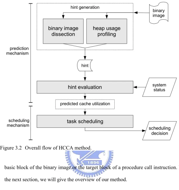
(25) hint generation. binary image dissection. binary image. heap usage profiling. prediction mechanism hint. hint evaluation. system status. predicted cache utilization. scheduling mechanism. task scheduling scheduling decision. Figure 3.2 Overall flow of HCCA method.. basic block of the binary image or the target block of a procedure call instruction. In the next section, we will give the overview of our method.. 3.2 Overview The scheduler requires predicting the memory access pattern of a task because the scheduling decision must be made before tasks being executed. Previous techniques usually predict the memory access behavior of a particular task according to its previous memory accesses. However, tasks may change their behaviors during their execution, so these techniques may result in false prediction and lead to an inferior scheduling decision. In order to obtain more accurate predictions, we propose the technique that directly analyzes the binary image of a task to figure out - 15 -.

(26) the memory access pattern. Because the processor is instructed by the binary image to accomplish the task, it is possible to predict the change of the behavior of tasks by analyzing their binary images. Therefore, we expect our proposed technique to bring more precisely predictions and make better scheduling decisions. The proposed technique is named Hint-aided Cache Contention Avoidance (HCCA). The overall flow of HCCA is shown in Figure 3.2, which contains three main phases. First, the hint generation phase will generate an abstract of binary image which contains necessary information to predict memory accesses. This phase includes two parts: binary image dissection and heap usage profiling. The binary image dissection part attempts to extract information from the binary image, which will be used to predict memory accesses on the code, static and stack partitions. We call this extracted information as hint. After profiling the task, the heap usage profiling part attempts to discover instructions that sequentially access memory from the execution trace. Addresses of these instructions will be recorded and stored into hint. Then, in the second phase, the hint evaluator will be activated when a task leaves the core. The hint evaluator predicts the future memory accesses of the leaving task by combining the hint and other factors such as program counter, addresses of allocated memory and addresses of call stack top. The predicted memory accesses are converted into cache set accesses according to the cache configuration. In the third phase, we attempt to avoid the cache contentions by assigning tasks using the same cache sets to the different gang. If there is any unscheduled gang in the gang queue, one of these will be selected for scheduling. Otherwise, tasks in the global dispatch queue are grouping into gangs for scheduling.. - 16 -.

(27) source. source. preprocessor. preprocessing. preprocessor. compiler. compiling. compiler. assembler. assembling. assembler. link-editor. linking. link-editor. hint generation. executable binary image. hint generater executable binary image. (a). hint. (b). Figure 3.3 The high level programming language processing flow. (a) The conventional processing flow. (b) The proposed processing flow.. 3.3 Hint generation Figure 3.3(a) illustrates the conventional processing flow, which is widely used in existing systems[25]. As shown in Figure 3.3(b), the hint generation resides after the linking processing of the high level language processing flow. Analyzing the binary image needs a lot of time. In order to speed up the prediction, we first extract the necessary information for the prediction in this phase. Without this phase, the prediction process will need unacceptable long time. As shown in Figure 3.2, this phase included two methods. We will describe the binary image dissection in section 3.3.1 and the heap usage profiling in section 3.3.2.. - 17 -.

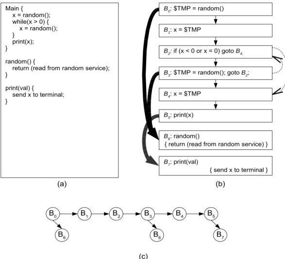
(28) Main { x = random(); while(x > 0) { x = random(); } print(x); }. B0: $TMP = random() B1: x = $TMP B2: if (x < 0 or x = 0) goto B4;. random() { return (read from random service); }. B3: $TMP = random(); goto B2;. print(val) { send x to terminal; }. B4: x = $TMP B5: print(x) B6: random() { return (read from random service) } B7: print(val). { send x to terminal }. (a). B0. (b). B1. B2. B3. B6. B4 B6. B5 B7. (c). Figure 3.4 An example of sibling-child binary tree representation of basic blocks.. 3.3.1. Binary image dissection This mechanism is designed to extract necessary information from the binary. image. This extracted information can be used to predict the memory accesses. First, we divide the code context of the binary image into basic blocks. Then, we extract the basic block characteristics that can assist the prediction. These extracted characteristics are described in the following. Let's consider a basic block Bi. We denote code(Bi) as an address set of instructions which are included in Bi. exp_time(Bi) is the expected execution time of Bi, which can be computed by summing the numbers of clock cycles executed by all instructions belong to Bi. static(Bi) is an address set of the accessed data which - 18 -.

(29) resides in the static partition. We can obtain these addresses from the binary image, because instructions which access to the static partition usually use immediate values to indicate their destinations. stack(Bi) is the memory size required to be allocated from the stack partition. The call stack is used to store the local data structures, such as local variables and call parameters. Therefore, the stack(Bi) can be obtained by counting how many local data structures which are allocated and used in Bi. next_bb(Bi) is used to indicate the basic block executed next to Bi. If Bi is the latest basic block of a procedure, next_bb(Bi) will be set to empty value. For example, as shown in Figure 3.4, next_bb(B3) is B4 and next_bb(B5) is empty. If Bi contains a procedure call instruction, then call_bb(Bi) will indicate the first basic block of the calling target. Otherwise, call_bb(Bi) will be set to empty value. For example, in Figure 3.4, call_bb(B3) is B6, and call_bb(B4) is empty value. In the following, we use a right-sibling left-child binary tree to represent the execution flow of the task. In this binary tree, a node represents a basic block, and an edge indicates the control dependency between two connected nodes. For every basic block Bi, we let call_bb(Bi) and next_bb(Bi) be the child and sibling node of Bi respectively. However, if the given task contains a recursive call, it will cause an edge loop in the right-sibling left-child binary tree. Hence, for the basic block Br which performs a recursive call, we set call_bb(Br) to empty value and merge Br into next_bb(Br). The corresponding right-sibling left-child binary tree of Figure 3.4(b) is shown in Figure 3.4(c).. 3.3.2. Heap usage profiling The execution of the same binary image with different input data may result in. - 19 -.

(30) different execution trace. In order to discover those memory-referencing instructions which have predictable behavior, we proposed a mechanism to analyze the collected execution trace after profiling. Before describing the detailed method of this analysis mechanism, we introduce the following terminologies. Considering a memory accesses ai, task(ai) is the task which performs ai, inst(ai) is the number of instructions which has been executed by task(ai) before ai. clkc(ai) is the number of elapsed clock cycles from the start of the execution of task(ai). addr(ai) is the memory address which ai accesses to. instruction(ai) is the memory-referencing instruction which performs ai. Definition 3.1 For sequence memory accesses A = {a1, a2, ... an} where a1, a2, ... an denote the individual accesses of A and they are performed by the same instruction. A is a sequential access if A satisfies the following conditions:. {. inst a i1 inst a i =inst  ai inst a i1 ... 1 where 2≤i≤ n1 , n≥3 addr  ai 1 addr a i =addr a i addr  ai 1 ... 2 An example of such instruction is a memory-referencing instruction within. loop block. If A satisfies the equation (1), it indicates that the number of instructions executed between any two contiguous memory accesses of A are the same. We denote the number of instructions between two contiguous memory accesses by ∆inst(A) if A satisfies the equation (1). If A satisfies the equation (2), it indicates that the address distance between any two contiguous memory accesses of A are the same. We denote the distance between two access targets by ∆addr(A) if A satisfies the equation (2). ∆clkc(A) denotes the average number of clock cycles between two contiguous accesses of A. ∆clkc(A) is calculated by formula 3.1.. - 20 -.

(31) n1. ∑ clkc a i1 clkc a i.  clkc  A= i =1. ..............................................................(3.1). n1. Now we describe our mechanism in detail. The proposed mechanism has two stages. The first stage of this analysis is to find the memory-referencing instructions that perform sequential accesses from the execution trace. We predict that these instructions will still perform sequential access. Other types of access patterns are simply ignored, because most of them do not have a determined pattern. This stage includes the following two steps. First, we extract all sequential accesses from the execution trace. Then, considering a memory-referencing instruction R which performs sequential accesses Ki, we predict that R will perform sequential access in the future if all ∆inst(Ki) have the same value and all ∆addr(Ki) have the same value for all sequential accesses Ki. For convenience, we denote the value of ∆inst(Ki) for R as inst_step(R) and denote the ∆addr(Ki) for R as addr_step(R). For R, we also predict the distance between two accessed addresses will be addr_step(R), and the number of clock cycles between two accessed addresses will be the averaged value of ∆clkc(Ki) in the future. For convenience, we denote the averaged value of ∆clkc(Ki) as clkc_step(R). We store the instruction address of R, clkc_step(R) and addr_step(R) as part of the hint. In the second stage, we attempt to find the memory-allocating instructions which allocate memory blocks for the memory-referencing instructions which perform sequential access. We predict that these memory-allocating instructions will still perform memory allocation for those memory-referencing instructions. This is done by comparing the accessed target of the memory-referencing instruction and the address range of allocated memory blocks. Considering a memory-referencing - 21 -.

(32) HeapUsageProfiling() SeqAccess ← NIL. // here we store the result of 1st stage. // 1st stage for each memory accessing event e do. // collect all memory accesses. SeqAccess[ instruction(e) ] ← SeqAccess[ instruction(e) ] ∪ { e}. for each instruction R where SeqAccess[R] exists do. B ← SeqAccess[R]. // remove those are not // sequential accesses. if ∃L: L = {K0, K1, ... Kn} where. ∀Ki, Kj ∈ L: Ki ∩ Kj = Ø, ∀Ki ∈ L: Ki is a sequential access, and ∪ K i=B. ∀ K i∈ L. then calculate clkc_step[R] and addr_step[R] else remove SeqAccess[R]. // 2nd stage for each memory allocating event e do. // check all memory allocations. if ∃a, ∃R: a ∈ K, K ∈ SeqAccess[R] where. allocation_start(e) ≤ addr(a) and allocation_end(e) ≥ addr(a) then allocating[R] ← allocating[R] ∪ { instruction(e) }. // finished, store hint Store Hint_H as the following set of vectors: ∀R where SeqAccess[R] is exist: <R, address[R], allocating[R], clkc_step[R], addr_step[R]> Figure 3.5 The algorithm of the heap usage profiling.. instruction R and a memory allocating instruction L, we predict that L will still allocate memory for R in the future. These referencing-allocating relations are stored as part of the hint. The algorithm of this mechanism is shown in Figure 3.5.. 3.4 Hint evaluation In the previous phase, we collect the hint which includes the information about how a task may use memory. In this phase, we predict the future memory usage for - 22 -.

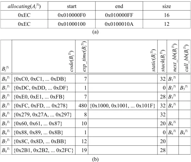
(33) B0Ti {0xC0, 0xC1, ... 0xDB}. 7. B1Ti {0xDC, 0xDD, ... 0xDF}. 1. B2Ti {0xE0, 0xE1, ... 0xFB}. 7. B3Ti {0xFC, 0xFD, ... 0x278}. call_bb(BjTi). next_bb(BjTi). stack(BjTi). static(BjTi). exp_time(BjTi). code(BjTi). BjTi. 32 B1Ti 0 B2Ti B5Ti 28 B3Ti. 96 {0x1000, 0x1001, ... 0x101F} 32 B4Ti. B4Ti {0x279, 0x27A, ... 0x297}. 8. 32. B5Ti {0x60, 0x61, ... 0x87}. 10. 20 B6Ti. B6Ti {0x88, 0x89, ... 0x8B}. 1. B7Ti {0x8C, 0x8D, ... 0xBB}. 12. 20. B8Ti {0x2B1, 0x2B2, ... 0x2FC}. 19. 28. 0 B6Ti B8Ti. (a) B0Ti. B1Ti. B2Ti. B5Ti. B3Ti. B6Ti. B4Ti. B7Ti. B8Ti (b) AjTi. address(AjTi). A0Ti 0x268. allocating(AjTi). addr_step(AjTi). 0xEC. clkc_step(AjTi) 4. 96. (c) Figure 3.6 An example of Hint. (a) Hint_B(Ti). (b) The binary tree representation of Hint_B(Ti). (c) Hint_H(Ti).. tasks when they leave cores by combining the hint and the task execution status. We first define some symbols in this phase. Considering a task Ti, we use GoingAccess(Ti) to represent the memory address set which may be accessed by the task Ti in the next time slice. StackTop(Ti) is the address of the top of the call stack. Hint_B(Ti) is the hint of Ti which is generated by the binary image dissection. BjTi is - 23 -.

(34) the basic block which is included by Hint_B(Ti) where 1≤ j ≤M, M is the number of basic blocks included in Hint_B(Ti). Hint_H(Ti) is the hint of Ti which is generated by the heap usage profiling. AkTi is one of the hint entries included in Hint_H(Ti) where 1≤ k ≤Q, Q is the number of entries included in Hint_H(Ti). Each hint entry represents one of the memory-referencing instructions which is predicted performing sequential accesses. We call such memory-referencing instructions as hint-covered memory-referencing instructions for convenience. address(AkTi) represents the address of AkTi. allocating(AkTi) is the address of the memory allocating instruction which allocate memory blocks for AkTi. addr_step(AkTi) is the distance between two accessed addresses. clkc_step(AkTi) is the number of clock cycles between two accesses. Figure 3.6 shows an example of the hint. For convenience, we denote the memory-referencing instruction located at address(AkTi) as instruction(AkTi). The hint evaluation has three stages. In the first stage, we predict the number of clock cycles will be used by the hint-covered memory-referencing instructions to access the dynamically allocated memory blocks. The prediction result is used to adjust the estimated execution time of a basic block which is estimated by the hint generation phase. In the hint generation phase, we do not know how large the dynamically allocated memory block will be. Therefore, it is impossible to predict how many clock cycles will be required for accessing the allocated memory blocks. However, in this phase, we can retrieve the memory allocation result from the memory allocation information maintained by the operating system. Therefore, we can estimate the number of clock cycles which is required for accessing the dynamically allocated memory blocks in this phase. Considering a task Ti and the. - 24 -.

(35) hint entry AkTi included in Hint_H(Ti), the prediction is done in two steps. First, we estimate how many times the instruction(AkTi) will be executed. This estimation can be made by dividing the size of the allocated memory block by addr_step(AkTi). Because we predict that the instruction(AkTi) will perform sequential accesses and the address distance between two contiguous accesses performed by instruction(AkTi) will be addr_step(AkTi). If there are multiple memory blocks that are allocated for instruction(AkTi) to access, we will perform the estimation with the size of the largest one for safety, because we do not know which one will be accessed. Then, we multiply the estimation result from previous step with clkc_step(AkTi) to make the prediction. We implement this two step prediction mechanism with formula 3.2. In this formula, MaxAllocSize(allocating(AkTi)) denotes the maximum allocated memory size which is allocated by allocating(AkTi). If there is no memory block allocated by allocating(AkTi), the value of MaxAllocSize(allocating(AkTi)) is zero. Ti k. dynAccessClk  A =. Ti. MaxAllocSize allocating  Ak  Ti k. addr _ step A . Ti. ×clkc _ step  Ak  .........(3.2). Then, the predicted number of clock cycles is used to adjust the expected execution time of basic blocks. Considering AkTi as one of the entries in Hint_H(Ti) and its corresponding basic block BjTi, the value of exp_time(BjTi) is adjusted by adding dynAccessClk(AkTi) to it. If there are multiple entries in Hint_H(Ti) which are mapped to a single basic block, we only select the maximum number of predicted clock cycles to add it. The value of exp_time(BjTi) will be restored after finishing this phase. An example of this adjustment is shown in Figure 3.7 which is the adjustment result of the example in Figure 3.6. The memory allocating result of A0Ti is shown in Figure 3.7(a). The corresponding basic block of A0Ti is B3Ti because address(A0Ti) is. - 25 -.

(36) allocating(AjTi). start. end. size. 0xEC. 0x010000F0. 0x010000FF. 16. 0xEC. 0x01000100. 0x0100010A. 12. B0Ti {0xC0, 0xC1, ... 0xDB}. 7. B1Ti {0xDC, 0xDD, ... 0xDF}. 1. B2Ti {0xE0, 0xE1, ... 0xFB}. 7. B3Ti {0xFC, 0xFD, ... 0x278} B4Ti {0x279, 0x27A, ... 0x297} Ti. call_bb(BjTi). 32 B1Ti 0 B2Ti B5Ti 28 B3Ti. 480 {0x1000, 0x1001, ... 0x101F} 32 B4Ti 8. 32 20 B6Ti. {0x60, 0x61, ... 0x87}. 10. B6Ti {0x88, 0x89, ... 0x8B}. 1. B7Ti {0x8C, 0x8D, ... 0xBB}. 12. 20. B8Ti {0x2B1, 0x2B2, ... 0x2FC}. 19. 28. B5. next_bb(BjTi). stack(BjTi). static(BjTi). BjTi. exp_time(BjTi). code(BjTi). (a). 0 B6Ti B8Ti. (b) Figure 3.7 An example of the expected execution time adjustment of basic blocks. (a) The allocation result of memory-allocating instruction at 0xEC (b) The adjusted Hint_B(Ti). included in code(B3Ti). The adjustment result of the expected execution time is shown in Figure 3.7(b) where the exp_time(B3Ti) is adjusted by adding the calculation result of formula 3.2. In the second stage, we predict the memory addresses that will be access by the task Ti in the upcoming allocated time slice. These predicted addresses are converted into the predicted cache set usage in the next stage. In this stage, we first find the corresponding basic block of the current execution point of the task. Then, we start a depth-first traversal from the corresponding basic block of the current execution point. That is, for every visited basic block BjTi, we first visit its child node - 26 -.

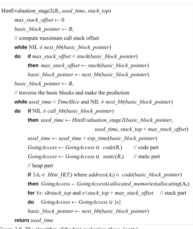
(37) HintEvaluation(Ti) GoingAccess ← Ø EstimatedDynAccessClk ← Ø // 1st stage for each entries Ak in Hint_H(Ti) do. tmp ← dynAccessClk(Ak) Locate hint entry Bj from Hint_B(Ti) such that address(Ak) ∈ code(Bj) if EstimatedDynAccessClk[Bj] is not existed or. EstimatedDynAccessClk[Bj] < tmp then EstimatedDynAccessClk[Bj] ← tmp for each Bj where EstimatedDynAccessClk[Bj] is existed do. exp_time(Bj) ← EstimatedDynAccessClk[Bj]. // 2nd stage Locate hint entry Bpc from Hint_B(Ti) such that ProgramCounter ∈ code(Bpc) HintEvaluation_stage2(Bpc, 0, StackTop(Ti)). // predict target addresses of // memory accesses. // 3rd stage Convert memory addresses included in GoingAccess into the cache set usage according to the cache configuration of the system. Output the converted result as the predicted cache set usage of Ti. Figure 3.8 The algorithm of the hint evaluation phase.. call_bb(BjTi). Then we visit its sibling node next_bb(BjTi). For every visited basic block BjTi, we copy the values in code(BjTi) and static(BjTi) into GoingAccess(Ti). We also add the addresses between StackTop(Ti) and StackTop(Ti)+stack(BjTi) into GoingAccess(Ti). The added addresses predict the usage of the stack partition. For memory-referencing instructions AkTi, when their corresponding basic blocks are traversed, the addresses of memory blocks which are allocated by allocating(AkTi) are also added into GoingAccess(Ti) to predict the usage of the heap part. The traversal is stopped when the summing of expected execution time of all traversed. - 27 -.

(38) HintEvaluation_stage2(Bx, used_time, stack_top) max_stack_offset ← 0 basic_block_pointer ← Bx // compute maximum call stack offset while NIL ≠ next_bb(basic_block_pointer) do. if max_stack_offset < stack(basic_block_pointer) then max_stack_offset ← stack(basic_block_pointer). basic_block_pointer ← next_bb(basic_block_pointer) basic_block_pointer ← Bx // traverse the basic blocks and make the prediction while used_time < TimeSlice and NIL ≠ next_bb(basic_block_pointer) do. if NIL ≠ call_bb(basic_block_pointer) then used_time ← HintEvaluation_stage2(basic_block_pointer,. used_time, stack_top + max_stack_offset) used_time ← used_time + exp_time(basic_block_pointer) GoingAccess ← GoingAccess ∪ code(Bx). // code part. GoingAccess ← GoingAccess ∪ static(Bx). // static part. // heap part if ∃Ak ∈ Hint_H(Ti) where address(Ak) ∈ code(basic_block_pointer) then GoingAccess ← GoingAccess∪ allocated_memories(allocating(Ak) for ∀s: s≥stack_top and s<stack_top + max_stack_offset do. // stack part. GoingAccess ← GoingAccess ∪ {s}. basic_block_pointer ← next_bb(basic_block_pointer) return used_time. Figure 3.9 The algorithm of the hint evaluation phase. (cont.). basic blocks is larger than the time slice. In the third stage, the predicted memory addresses are converted into predicted cache set usage. Therefore, in the task scheduling phase, we can attempt to avoid cache contentions by not concurrently scheduling tasks which use the same cache sets on cores. Considering a m-set cache and a task Ti, the predicted cache accesses. - 28 -.

(39) of Ti is represented in a bit vector <C1Ti, C2Ti, ..., CmTi>. CbTi represents the predicted usage of the bth cache set. The bth cache set is predicted to be used if there is a memory address included in GoingAccess(Ti) which is mapped to it. If the bth cache set is predicted to be used, the value of Cb will be set to 1. Otherwise Cb will be set to 0. The algorithm of this phase is shown in Figure 3.8 and Figure 3.9.. 3.5 Task scheduling In the previous phase, the cache set usage of a task is predicted. In this phase, we group tasks in the global dispatch queue into small gangs according to their predictions of the cache usages and store gangs into the gang queue for future scheduling. When the scheduler is activated by idle cores, the scheduler will randomly pick one gang from the gang queue and assign tasks in the gang to the cores. For each gang, the number of contained tasks is no more than the number of cores within the system. The number of gang is equal to the following formula. In this formula, TaskCount denotes the number of tasks in the system. CoreCount denotes the number of cores in the system. GangCount=⌈. TaskCount ⌉ ............................................................................. (3.3) CoreCount. Before we describing the detailed mechanism of this phase, we first introduce the following formulas and terminologies which are used in this phase. Formula 3.4 is used to predict the number of cache contentions between two tasks. m. PredictedCacheContention T i , T j =∑ C Tk ×C Tk  ....................................... (3.4) i. j. k=1. In this formula, Ti and Tj are two tasks, m is the number of cache sets. CkTi and CkTj represent the predicted usage of the kth cache set of Ti and Tj which are described in - 29 -.

(40) the previous section. Considering two tasks Ti and Tj, we multiply CkTi with CkTj to see if both Ti and Tj are predicted to use the kth cache set. If both Ti and Tj are predicted to use the kth cache set, as we described in the previous section, both the value of CkTi and CkTj will be one. Therefore, the multiplication result will be one which indicates one predicted cache contention. However, if none of Ti and Tj are predicted to use the kth cache set or only one of Ti and Tj is predicted to use the kth cache set, at least one of CkTi and CkTj will be zero. Therefore, the multiplication result will be zero which indicates no cache contention. By summing all multiplication results on m cache sets, we can get the number of predicted cache contentions between Ti and Tj. Furthermore, formula 3.5 predicts the number of cache contentions between a task and tasks of a gang. TaskGangCacheContentionT i ,G x =. ∑ ∀ T j ∈G x. PredictedCacheContention T i , T j . ................................................................................................... (3.5) In this formula, Ti is a task and Gx is a gang. The number of cache contentions between Ti and tasks of Gx is predicted by summing the number of predicted cache contentions between Ti and each task included in Gx. The number of predicted cache contentions between two tasks can be got by applying formula 3.4. We use formula 3.5 to see if a task and a gang are perfect matching or not. Considering a task Ti and a gang Gx, if Ti and Gx are perfect matching, we can assign Ti into Gx without introducing any predicted cache contentions with other tasks within Gx. We say that Ti and Gx are perfect matching if the value of TaskGangCacheContention(Ti, Gx) is zero. Otherwise, we say that Ti and Gx are not perfect matching. There are two stages in our gang grouping mechanism. In the first stage, the tasks with the largest number of predicted used cache sets will be distributed into - 30 -.

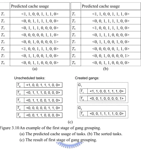
(41) Predicted cache usage. Predicted cache usage. T1. <1, 1, 0, 0, 1, 1, 1, 0>. T1. <1, 1, 0, 0, 1, 1, 1, 0>. T2. <0, 0, 1, 1, 1, 1, 0, 0>. T2. <0, 0, 1, 1, 1, 1, 0, 0>. T3. <0, 1, 1, 1, 0, 0, 0, 0>. T6. <1, 0, 0, 1, 1, 1, 0, 0>. T4. <0, 0, 0, 0, 0, 1, 1, 0>. T3. <0, 1, 1, 1, 0, 0, 0, 0>. T5. <0, 0, 1, 0, 0, 0, 0, 1>. T7. <0, 1, 1, 0, 0, 1, 0, 0>. T6. <1, 0, 0, 1, 1, 1, 0, 0>. T4. <0, 0, 0, 0, 0, 1, 1, 0>. T7. <0, 1, 1, 0, 0, 1, 0, 0>. T5. <0, 0, 1, 0, 0, 0, 0, 1>. T8. <0, 0, 1, 1, 0, 0, 0, 0> (a). T8. <0, 0, 1, 1, 0, 0, 0, 0> (b). Unscheduled tasks:. Created gangs:. T6. <1, 0, 0, 1, 1, 1, 0, 0>. T3. <0, 1, 1, 1, 0, 0, 0, 0>. T1. <1, 1, 0, 0, 1, 1, 1, 0>. T7. <0, 1, 1, 0, 0, 1, 0, 0>. T5. <0, 0, 1, 0, 0, 0, 0, 1>. T4. <0, 0, 0, 0, 0, 1, 1, 0>. T8. <0, 0, 1, 1, 0, 0, 0, 0>. G1. G2 T2. <0, 0, 1, 1, 1, 1, 0, 0>. (c) Figure 3.10 An example of the first stage of gang grouping. (a) The predicted cache usage of tasks. (b) The sorted tasks. (c) The result of first stage of gang grouping.. different gangs. Therefore, the possibility of the occurrence of cache contentions could be reduced. In this stage, we first sort tasks according to the number of predicted used cache sets in the decreasing order. Then we distribute tasks into gangs. The first gang is created by assigning the task with most predicted used cache sets to an empty gang. The remaining tasks are assigned to a gang one by one according to the number of predicted used sets. Considering a task Ti and a gang Gx, Ti will be assign to Gx if Ti and Gx are perfect matching. If there is no such gang exists and the number of the created gang is less than GangCount, a new gang will be created and Ti will be assigned to the created gang. If there is no such gang which. - 31 -.

(42) G1. G1. T1. <1, 1, 0, 0, 1, 1, 1, 0>. T1. <1, 1, 0, 0, 1, 1, 1, 0>. T5. <0, 0, 1, 0, 0, 0, 0, 1>. T5. <0, 0, 1, 0, 0, 0, 0, 1>. T3. <0, 1, 1, 1, 0, 0, 0, 0>. T4. <0, 0, 0, 0, 0, 1, 1, 0>. TaskGangCacheContention(T6, G1)=3 T6. <1, 0, 0, 1, 1, 1, 0, 0>. G2. TaskGangCacheContention(T6, G2)=3 G2 T2. <0, 0, 1, 1, 1, 1, 0, 0>. T2. <0, 0, 1, 1, 1, 1, 0, 0>. T6. <1, 0, 0, 1, 1, 1, 0, 0>. T7. <0, 1, 1, 0, 0, 1, 0, 0>. T8. <0, 0, 1, 1, 0, 0, 0, 0>. (b). (a). Figure 3.11 An example of the second stage of gang grouping. (a) The assignment of T6. (b) The final result of gang grouping.. exists and the number of gangs is equal to GangCount, the assignment of Ti will be left to the next stage. Figure 3.10 shows an example of this stage. Assuming there is an 8-sets L2 cache and two cores in the system. There are 8 tasks in the system, therefore the value of GangCount is 2. After the previous stage, a task may still remain to be assigned if the task can not form any perfect matching with created gangs and the number of created gangs is equal to GangCount. We distribute the remaining tasks into gangs in the second stage. In the second stage, the remaining tasks are assigned to gangs one by one according to the number of predicted used cache sets. Each remained task is greedily assigned to a gang which creates the lowest number of predicted cache contentions with other tasks within the gang. We expect the overall assignment will cause the least number of cache contentions, because we introduce the least number of predicted cache contention for each assignment. Considering a task Ti, we first - 32 -.

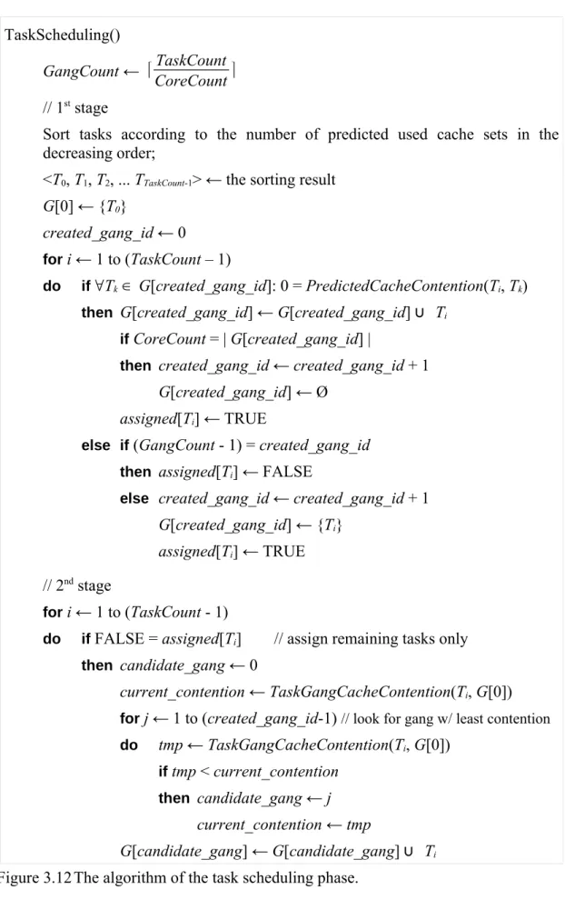
(43) TaskScheduling() GangCount ← ⌈. TaskCount ⌉ CoreCount. // 1st stage Sort tasks according to the number of predicted used cache sets in the decreasing order; <T0, T1, T2, ... TTaskCount-1> ← the sorting result G[0] ← {T0} created_gang_id ← 0 for i ← 1 to (TaskCount – 1) do. if ∀Tk ∈ G[created_gang_id]: 0 = PredictedCacheContention(Ti, Tk) then G[created_gang_id] ← G[created_gang_id] ∪ Ti if CoreCount = | G[created_gang_id] | then created_gang_id ← created_gang_id + 1. G[created_gang_id] ← Ø assigned[Ti] ← TRUE else if (GangCount - 1) = created_gang_id then assigned[Ti] ← FALSE else created_gang_id ← created_gang_id + 1. G[created_gang_id] ← {Ti} assigned[Ti] ← TRUE // 2nd stage for i ← 1 to (TaskCount - 1) do. if FALSE = assigned[Ti]. // assign remaining tasks only. then candidate_gang ← 0. current_contention ← TaskGangCacheContention(Ti, G[0]) for j ← 1 to (created_gang_id-1) // look for gang w/ least contention do. tmp ← TaskGangCacheContention(Ti, G[0]) if tmp < current_contention then candidate_gang ← j. current_contention ← tmp G[candidate_gang] ← G[candidate_gang] ∪ Ti Figure 3.12 The algorithm of the task scheduling phase.. - 33 -.

(44) calculate the number of predicted cache contentions of Ti and every existing gangs. For gang Gx, the number of predicted cache contentions between Gx and Ti is calculated by formula 3.5. Then, Ti is assigned to the gang which has the smallest number of predicted cache contentions between the gang and Ti. If there are multiple gangs which have the same number of predicted cache contentions with Ti, the gang with fewer tasks will be selected. Figure 3.11 shows the second stage of gang grouping for the example which is illustrated in Figure 3.10. Figure 3.11(a) shows the assignment of T6, where the number of cache contentions between T6 and both gangs are the same. But, G2 has the less number of tasks. Therefore, T6 is assigned to G2. Figure 3.11(b) shows the final result of the gang grouping. The algorithm of this phase is shown in Figure 3.12. So far, we have introduced the essence of our mechanism. In the next chapter, we will evaluate the performance of our mechanism and compare with others.. - 34 -.

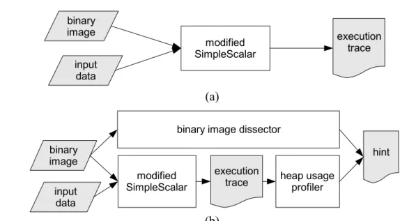
(45) Chapter 4 Preliminary Performance Evaluation In this chapter, we will demonstrate our experimental results. The architecture of simulator and evaluated workloads are described in section 4.1. The evaluation results are shown in section 4.2.. 4.1 Simulation overview Before executing the simulation, we first use a modified SimpleScalar[26] to collect the execution trace of tasks. The trace collecting process is diagrammed at Figure 4.1(a). The hints are also generated before executing the simulation. As shown in Figure 4.1(b), our hint generator contains a binary image dissector and a heap usage profiler to simulate the hint generation phase of HCCA (Hint-aided Cache Contention Avoidance). Then, the execution traces and hints are sent to our simulator. binary image. execution trace. modified SimpleScalar. input data. (a) binary image dissector binary image input data. hint modified SimpleScalar. execution trace. heap usage profiler. (b) Figure 4.1 The trace generator and the hint generator. (a) The trace generator. (b) The hint generator. - 35 -.

(46) execution trace 1. execution trace 2. execution trace N. trace parser. trace parser. trace parser. hint 1 scheduling method simulator. hint 2. HCCA Hint evaluator RoundRobin. hint N. ActiveSet. TOS. Task scheduler. memory simulator. Figure 4.2 The architecture of our simulator.. Figure 4.2 shows the architecture of our simulator which contains three modules: trace parser, scheduling method simulator, and memory simulator. The trace parser extracts memory access events from the execution trace. The extracted events are sent to the scheduling method simulator. In addition to memory access events, values of registers and results of memory allocating operations are also extracted by the trace parser for HCCA. The scheduling method simulator makes the scheduling decisions. For tasks which are selected by the scheduling method simulator to be active tasks, the corresponding memory access events received from the trace parser are forwarded to the memory simulator by the scheduling method simulator. Otherwise, those memory access events will be queued at the scheduling method simulator. For the comparisons among different task scheduling methods, we have to implement different scheduling methods in the scheduling method. - 36 -.

(47) Parameter. Values. Number of cores size associativity L1 I-cache. line size miss latency replacement policy size associativity. L1 D-cache. line size miss latency replacement policy size associativity. L2 cache. line size miss latency replacement policy. 4 32 KB 2 32 bytes 10 cycles LRU 32 KB 2 16 bytes 10 cycles LRU 2 MB 4, 8, 16 32 bytes 81 cycles LRU. Figure 4.3 The configuration of memory simulator. simulator. The following methods are implemented: Round-Robin[18], ActiveSet[14],. TOS. (Throughput-oriented. Scheduling)[15]. and. HCCA.. The. implementation of HCCA contains a hint evaluator and a task scheduler which simulate the hint evaluation phase and the task scheduling phase respectively. The corresponding hints of tasks and all trace events from the trace parser except memory access events are sent to the hint evaluator. The memory access events are sent to the task scheduler. The memory simulator simulates the memory hierarchy. The accessing hit and miss events of L2 cache are sent to the scheduling method simulator for Active-Set and TOS. In our simulation, we simulate a four core chipmultiprocessor system. Figure 4.3 shows the cache configuration of our simulation. This configuration is based on the configuration of MIPS R10000 processor used in - 37 -.

(48) ammp. art-110. art-470. bzip2-graphic. bzip2-program. bzip2-random. bzip2-source. equake. gcc-166. gcc-200. gcc-expr. gcc-integrate. gcc-scilab. gzip-graphic. gzip-program. gzip-random. gzip-source. mcf. mesa. vortex-lendian1. vortex-lendian2. vortex-lendian3. vpr-place. vpr-route. Figure 4.4 The list of tasks used in our simulation.. the SGI Origin200 workstation[27, 28]. We want to evaluate how the associativity of L2 cache may affect our method. Therefore, we simulate three different L2 cache associativity configurations. We simulate eight hundred million instructions for each task. The length of the time slice is set to ten million cycles for all evaluated task scheduling methods[14]. The simulation workload is formed by a set of tasks. We use benchmark programs and corresponding input data sets included in SPEC CPU2000[16] to form our workloads. A task is formed by a benchmark program and one of its input data set. Tasks are named by hyphening the name of the benchmark program and the name of the input data set. For example, the benchmark program gzip has four input data sets: graphic, program, source and random. Therefore, we form the following four tasks with gzip and its input data sets: gzip-graphic, gzip-program, gzip-source and gzip-random. Two input data sets may have the same name if they are used in different benchmark programs. The list of tasks used in our simulation is shown in Figure 4.4. For each benchmark program, a separated training data set is used as the input data of the hint generator to generate the hints. In our simulation, each workload includes twelve tasks. We form three workloads to evaluate the performance of our mechanism. We want to evaluate the performance of our. - 38 -.

(49) art-470 art-110 gzip-program gzip-random gzip-source gzip-graphic bzip2-program bzip2-graphic bzip2-random bzip2-source ammp mcf vortex-lendian1 vortex-lendian3 vortex-lendian2 gcc-166 gcc-expr gcc-200 gcc-integrate gcc-scilab mesa equake vpr-place vpr-route 0. 500000. 1500000. 2500000. 3500000. 4500000. 5500000. number of cache misses. Figure 4.5 The sorted task list. ammp. art-110. art-470. bzip2-graphic. bzip2-random. bzip2-source. mcf. gzip-graphic. gzip-program. gzip-random. gzip-source. ammp. bzip2-graphic. bzip2-program. gcc-166. gzip-graphic. gzip-program. mcf. vortex-1. vortex-2. vpr-place. vpr-route. equake. gcc-166. gcc-200. gcc-expr. gcc-scilab. mesa. vortex-lendian1. vortex-lendian3. vpr-place. vpr-route. Workload 1 bzip2-program. Workload 2 gcc-expr. Workload 3 gcc-integrate vortex-lendian2. Figure 4.6 The simulation workloads.. mechanism under the different possibility of the occurrence of cache contention. The tasks which frequently cause cache misses may cause more cache contentions[11, 15]. Therefore, we form our workloads according to the number of cache misses caused by individual tasks. We first execute the tasks once for eight hundred million cycles and sort tasks according to the number of cache misses in the decreasing order. The sorting result of our tasks is shown in Figure 4.5. Then, we form the. - 39 -.

(50) workloads according to the sorting result. Figure 4.6 shows our three kinds of workloads. Workload 1 is formed by selecting the first twelve tasks from the sorted task list which have more number of cache misses. Workload 2 is formed by randomly selecting six tasks from the first half of the sorted task list and randomly selecting another six tasks from the second half of the sorted task list. Workload 3 is formed by selecting the last twelve tasks from the sorted task list which have less number of cache misses.. 4.2 Evaluation results In the following subsections, we will first compare the cache set usage prediction accuracy of HCCA with Active-Set. Next, we will compare the L2 cache miss rate of HCCA with Round-Robin, Active-Set and TOS. Then, we will evaluate the overall performance improvement of HCCA.. 4.2.1. Prediction accuracy Both HCCA and Active-Set attempt to avoid cache contentions by separately. scheduling the tasks which are predicted to use the same cache set. Therefore, the accuracy of cache set usage prediction has a great effect on the performance of contention avoidance. The prediction accuracy is the percentage of cache set usage predictions which correctly predict the actual cache set usage. In order to obtain the prediction accuracy, we execute tasks alone in our simulator and compare the cache set usage predictions made by the task scheduler with the actual cache set usage. Figure 4.7 shows the prediction accuracy of Active-Set and HCCA for individual tasks. For most of tasks, HCCA performs better than Active-Set. For tasks that. - 40 -.

(51) 90% 80%. accuracy. 70% 60% 50% 40%. Hint Active-Set. 30%. ammp art-110 art-470 bzip2-graphic bzip2-program bzip2-random bzip2-source equake gcc-166 gcc-200 gcc-expr gcc-integrate gcc-scilab gzip-graphic gzip-program gzip-random gzip-source mesa vortex-lendian1 vortex-lendian2 vortex-lendian3 vpr-place vpr-route. 20%. benchmark. Figure 4.7 The prediction accuracy.. HCCA performs worse than Active-Set, we inspect the source code of such tasks for the causes of inferior predictions. After inspecting the source code of the binary images of these tasks, we realize that such tasks heavily use data structures which require irregular accesses within the heap part. However, HCCA does not predict such accesses.. 4.2.2. L2 miss rate Figure 4.8 shows the simulation result of workload 1. Figure 4.8(a) shows the. simulated L2 miss rate. Figure 4.8(b) shows the improvement over Round-Robin. We use Round-Robin as the baseline for comparison, because it does not contain any cache contention reduction mechanism. The simulation result shows that HCCA performs better than others. In workload 1, all three methods perform better under higher associativity. Figure 4.9 shows the simulation result of workload 2. The simulation result of workload 2 is similar to the result of workload 1 but with more improvement over Round-Robin. Figure 4.10 shows the simulation result of - 41 -.

(52) 8% RoundRobin Active-Set TOS HCCA. miss rate. 25.5%. 25.0%. improvement over Round-Robin. 26.0%. Active-Set TOS HCCA 6%. 4%. 2%. 24.5%. 0% 4-way. 24.0% 4-way. 8-way. 16-way. 8-way. associativity. 16-way. (b). (a). Figure 4.8 The simulation result of workload 1. (a) The L2 miss rate under various associativity configuration. (b) The percentage of improvement over Round-Robin.. RoundRobin Active-Set TOS HCCA. miss rate. 13.5%. 13.0%. 8%. improvement over Round-Robin. 14.0%. 6%. 4%. 2% Active-Set TOS HCCA. 12.5%. 0% 4-way. 12.0% 4-way. 8-way. 8-way. associativity. 16-way. (b). (a). Figure 4.9 The simulation result of workload 2. (a) The L2 miss rate under various associativity configuration. (b) The percentage of improvement over Round-Robin.. - 42 -. 16-way.

(53) 8% RoundRobin Active-Set TOS HCCA. miss rate. 1.5%. 1.0%. 0.5%. improvement over Round-Robin. 2.0%. 6%. 4% Active-Set TOS Hint 2%. 0% 4-way. 0.0% 4-way. 8-way. 16-way. 8-way. associativity. 16-way. (b). (a). Figure 4.10 The simulation result of workload 3. (a) The L2 miss rate under various associativity configuration. (b) The percentage of improvement over Round-Robin.. workload 3. Workload 3 is formed by tasks with less number of cache misses. In workload 3, HCCA still performs better than others. However, as shown in Figure 4.10(b), comparing to workload 1 and workload 2, we have the lower percentage of improvement over Round-Robin at the higher cache associativity. As shown in Figure 4.10(a), the reduced miss rate is similar in all three methods. Comparing to the simulation result of workload 1 and workload 2, the reduced miss rate is relatively small. In summary, for workload 1 and workload 2, we will have better cache miss improvement under higher associativity. This result is expected because the cache misses caused by cache contentions belong to conflict miss. The conflict misses can be further reduced under higher associativity[29]. However, for workload 3, the effect of cache contention is low enough and limits the further improvement of cache miss. All evaluated task scheduling methods may not be able to have better improvement under higher associativity for such workload. - 43 -.