國 立 交 通 大 學
土木工程學系
博 士 論 文
多頻道表面波震測之施測與頻散分析標準化研究
Towards the standardization of field testing and dispersion
analysis of MASW method
研 究 生:張宗盛
指導教授:林志平 教授
Towards the standardization of field testing and dispersion
analysis of MASW method
研 究 生:張宗盛 Student:Tzong-Sheng Chang
指導教授:林志平 Advisor:Chih-Ping Lin
國 立 交 通 大 學
土 木 工 程 學 系
博 士 論 文
A ThesisSubmitted to Department of Civil Engineering College of Engineering
National Chiao Tung University in partial Fulfillment of the Requirements
for the Degree of Doctor of Philosophy
in
Civil Engineering July 2009
HsinChu, Taiwan, Republic of China
多頻道表面波震測之施測與頻散分析標準化研究
學生:張宗盛 指導教授:林志平博士
國立交通大學土木工程學系
中文摘要
由於非破壞性的試驗方法及簡便操作等特性,將表面波震測運用於工址調查實務上 愈來愈受歡迎。特別是多頻道表面波震測(Multi-station Analysis of Surface Wave, MASW)紀錄針對單一測線可提供較深探測深度及較多資料。但如欲得到品質良好且寬 頻的頻散曲線,試驗施作時之施測參數即扮演一重要角色。選用施測參數時常因訊號分 析、施測解析度及深度上的不同考量而陷入兩難。除此之外,MASW 試驗者亦常對前 人提出之數種頻散分析演算方法進行驗證比較。本文最主要的課題即為針對 MASW 中 野外施測及頻散分析兩部分提出一標準步驟。針對野外施測,本文先行討論時間及空間 施測參數對實驗的影響,包含時間與空間域上的映頻與資料遺漏、波場的遠近場效應、 高次震態模組的影響及空間水平解析度等。之後針對各種影響加以探討分析並提出一創 新施測方式及合成震測資料方法,藉以消彌各施測參數選用規則上的衝突並使 MASW 施測步驟標準化而有利一般工地實務應用。在頻散分析方面,本文提出一波場轉換之統 一演算法。先將野外收錄之時間-空間域之二維波場轉換至頻率-空間域,並以線性迴歸 之多頻道表面波頻譜分析(Multi-channel Spectral Analysis of Surface Wave, MSASW)進 行初步頻散分析。透過頻率-空間域之複數頻譜及線性迴歸資料評估收錄訊號品質並消 除不良訊號。再將頻率-空間域之複數頻譜以統一波場轉換方式同時得到頻率-波數
(wavenumber)域、頻率-慢度(slowness)域、頻率-速度(velocity)域及頻率-波長 (wavelength)域之頻散曲線。本文並提出一藉由使用離散空間傅立葉轉換(discrete-space Fourier Transform)之最佳化方法證明各域之頻散曲線皆為相同,並討論頻散曲線取樣 時以等頻率及等波長進行之優劣。本文的各項結果可作為日後多頻道表面波震測實驗標 準化之基礎。
Towards the standardization of field testing and dispersion
analysis for MASW methods
Student:Tzong-Sheng Chang Advisors:Dr. Chih-Ping Lin
Department of Civil Engineering National Chiao Tung University
ABSTRACT
The surface wave method has gained popularity in engineering practice for determining S-wave velocity depth profiles. In particular, MASW (multi-station analysis of surface wave) method permits a single survey of a broad depth range and high levels of redundancy with a single field configuration. Despite its apparent advantage over the two-channel SASW (spectral analysis of surface wave) method, the testing configuration of the MASW method remains a crucial factor that may affect the test results. Tradeoffs are involved when selecting the testing parameters. In addition, several algorithms with different preferences in the literature exit for the dispersion analysis. The objectives of this study are to establish a standard procedure for field testing and dispersion analysis of MASW. In the field testing, the influences of temporal and spatial parameters were investigated, including aliasing and leakage in both time and space domain, far and near field effects, effect of higher modes, and horizontal resolution. The investigation leads to several rules for choosing testing parameters. An innovative testing procedure and the associated signal processing was proposed to resolve the dilemma of choosing testing parameters and standardize the testing procedure. In the dispersion analysis, a unified approach was proposed. The wavefield in time-space (t-x)
domain is transformed to frequency-space (f-x) domain first, in which a preliminary dispersion analysis (a new method called multi-channel spectral analysis of surface wave, MSASW) was introduced and methods for assessing data quality and data screening were proposed. The f-x domain is further transformed to f-k (wavenumber), f-p (slowness), f-v (velocity), or f-λ (wavelength). The dispersion curves obtained by different transformation are shown to be identical by a newly-proposed optimization method based on the discrete-space Fourier Transform, which allows the transformed domain remain continuous for best resolution of dispersion analysis. A wavelength-controlled sampling approach was further proposed for the dispersion curve to avoid bias in depth sampling. The results of this study may lead to further standardization of the surface wave testing.
誌
謝
如果不是指導老師林志平博士的引見、啟發及教導,我絕對無法來到交大開始我的 博士研究及完成本文。之於本文,林老師除了提供許多原創性的研究方向外,更在研究 邏輯及方法上不斷給我指引。如果說,本文對相關課題有一點點的貢獻,那我只是站在 林老師的肩膀上發現了這些結果。在此,我必須對他致上最高的謝意及敬意。 另外,在交大求學期間,我很榮幸地接受了許多老師指導。特別是潘以文教授及廖 志中教授亦師亦友的教誨,除了給我開闊眼界的知識外,也端正了我的人生觀,在此致 上由衷謝意。 論文口試期間,承蒙莊長賢教授、倪勝火教授、張文忠教授、余騰鐸教授、董家鈞 教授、潘以文教授及廖志中教授撥空蒞臨指導並給予寶貴意見,使我獲益良多,在此亦 致上敬意。 翔益營造的龔書潭及黃金煌兩位先生在這幾年給我極大的空間及時間,並讓我在經 濟上無後顧之憂,無以回報的我僅能致上感謝。另外,來到交大後,許多學長姐及學弟 妹都慷慨地提供協助。年近中年,還能交到許多真心相待的朋友,我想這是一個比學位 更重要的收穫。 我的家人給我的支持與鼓勵一直是我最有力的後盾。在交大的八年,我經歷了人生 中許多重大的起伏轉折。工作的忙碌奔波、研究的無力枯燥與生活的煩瑣枝節交互壓迫 下,常常讓我想要放棄研讀。然而,家人們、老師們、長官們及同學朋友們,你們持續 從不間斷的鼓勵讓我能完整地畫下句點,而不以逃避作為收場。我想,這個過程賦予我 人生的焠鍊、改變及意義遠遠大於博士學位所能帶來的小小虛榮。 謝謝你們!Contents
中文摘要...I ABSTRACT ... III
誌 謝... V Contents...VI
List of figures ...IX
List of tables ... XII
1 Introduction ... 1
1.1 Motivation... 1
1.2 Objectives ... 3
1.3 Dissertation outline ... 4
2 Literature review ... 6
2.1 Dynamic properties of soil and testing methods... 6
2.1.1 Dynamic properties of soil ... 6
2.1.2 Testing methods ... 10
2.2 Wave propagation and computation of surface wave ... 15
2.2.1 Basic theory of elastic wave propagation... 16
2.2.2 Computation of theoretical dispersion curve... 29
2.2.3 Computation of synthetic wavefield ... 33
2.3 Seismic tests using surface wave ... 36
2.3.1 Overview of surface wave methods ... 36
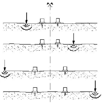
2.3.2 Field testing procedure of MASW ... 43
2.3.3 Dispersion analysis of MASW... 44
3 Investigation of field parameters and standardization of field testing ... 53
3.1 Temporal parameters of field testing ... 54
3.1.1 Aliasing due to time domain discretization: the sampling interval, Δt... 54
3.1.2 Leakage due to time domain truncation: total sampling duration, T ... 54
3.2 Spatial parameters of field testing... 55
3.2.1 Aliasing due to space domain discretization: the geophone spacing, Δx... 55
3.2.2 Leakage due to space domain truncation and modal separation: the geophone spread, L.... 57
3.2.3 Near and far field effects: the minimum offset, X0 and maximum offset, (X0+L) ... 60
3.2.4 The dilemma ... 62
3.3 The countermeasure: Pseudo-section approach ... 64
3.3.1 The concept of Pseudo-section method... 64
3.3.2 Combining seismic records of the pseudo-section method ... 66
3.3.3 Observation on near and far field effects via pseudo-section method... 72
3.4 Seismic sources and receivers... 74
3.4.1 Some improvement on the seismic source ... 74
3.4.2 Some improvement on the receivers ... 82
3.5 The proposed standard field testing... 89
4 Unified dispersion analysis ... 91
4.1 Analyses in the frequency-space (f-x) domain ... 93
4.1.1 Representation of surface waves in f-x domain... 93
4.1.2 Real part and energy spectrum of the f-x complex data ... 95
4.1.3 Phase Angles: Multi-station spectral analysis of surface wave (MSASW)... 95
4.1.4 Amendment for near and far field effect: Optimum offset range selection... 101
4.2 Unified Wavefield Transformation (UWFT)... 109
4.2.1 Different transformations and presentations of space domain ... 109
4.2.2 Characteristics of wavefield transformation in different domains ... 111
4.2.3 Optimization of dispersion analysis ... 124
4.4 The proposed standard dispersion analysis... 132
5 Conclusion and suggestion... 134
5.1 Conclusion... 134
5.2 Suggestion... 138
List of figures
Fig. 2-1 Cause-effect relationships in soil response to dynamic excitations... 6
Fig. 2-2 Dependence of threshold shear strains from plasticity index... 8
Fig. 2-3 Ranges of variability of cyclic shear strain amplitude in laboratory and in-situ tests... 10
Fig. 2-4 Stress notation of an element in an x-y-z Cartesian coordination ... 16
Fig. 2-5 The ratio of Rayleigh wave velocity, vR, verse body wave velocities as a function of Poisson ratio,ν ... 25
Fig. 2-6 Rayleigh wave particle motion in a homogeneous, isotropic half space; retrograde at the surface, passing through purely vertical at about λ/5 then becoming prograde at depth... 25
Fig. 2-7 Particle motions of Rayleigh wave over one wavelength along the surface and as a function of depth ... 26
Fig. 2-8 The model of a vertically heterogeneous halfspace... 26
Fig. 2-9 Rayleigh waves dispersion curves in vertically heterogeneous media... 30
Fig. 2-10 Rayleigh displacement eigenfunctions in vertically heterogeneous media... 30
Fig. 2-11 Typical dispersion curves of different type of strata... 32
Fig. 2-12 Steady State Rayleigh Wave (SSRW) method: field procedure ... 37
Fig. 2-13 Simplified inversion process proposed for the SSRM... 37
Fig. 2-14 SASW method field configuration... 38
Fig. 2-15 Common receiver midpoint array with source position reversing ... 39
Fig. 2-16 Common source array... 39
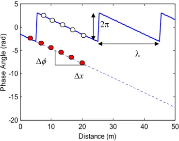
Fig. 2-17 SASW signal processing- Δφ vs Frequency ... 40
Fig. 2-18 Scheme of MASW... 42
Fig. 2-19 Field test configuration of MASW ... 44
Fig. 2-20 An example of f-k transformation ... 46
Fig. 2-21 Exemplification of the Slant-Stack transform concept... 47
Fig. 2-22 An example of p-f transformation ... 47
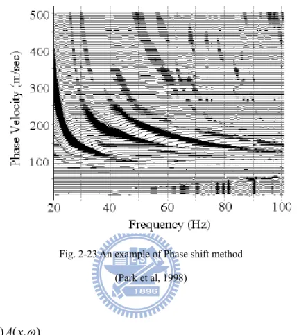
Fig. 2-23 An example of Phase shift method... 49
Fig. 2-24 Ratio a that was used during construction of the initial vs profiles ... 51
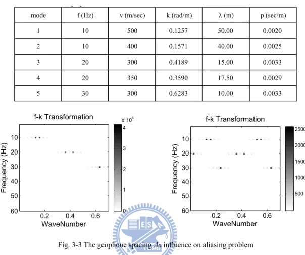
Fig. 3-2 An illustration of phase un-wrapping in the space domain for the multi-station spectral analysis of
surface wave... 55
Fig. 3-3 The geophone spacing Δx influence on aliasing problem ... 56
Fig. 3-4 The geophone spread L affects the modal separation... 57
Fig. 3-5 An example wavefield of a multi-mode surface wave ... 59
Fig. 3-6 Effects of multiple modes on the phase angle as a function of the source-to-receiver offset. ... 59
Fig. 3-7 Illustration of Pseudo-section method... 64
Fig. 3-8 Static errors in φ–x domain... 66
Fig. 3-9 Scheme of signal process for correction of the static error when seaming seismic records for synthesis of pseudo-section ... 67
Fig. 3-10 Dispersion curves from conventional and pseudo-section records analyzed by (a) Unified WaveField Transformation (UWFT) (b) Multi-channel Spectral Analysis of Surface Wave (MSASW) ... 70
Fig. 3-11 Phase angle difference of conventional and pseudo-section records ... 71
Fig. 3-12 Near and far field effects observed inφ–x domain ... 73
Fig. 3-13 Electrical operated seismic source ESS100SC... 75
Fig. 3-14 New developed weight-drop seismic source... 76
Fig. 3-15 The pseudo-section record by the source of the12 lb sledgehammer (BH) ... 79
Fig. 3-16 The pseudo-section record by the source of the spring accelerator (AF)... 80
Fig. 3-17 The pseudo-section record by the source of the new developed weight-drop source (WD)... 81
Fig. 3-18 The pedestals and receiver of the land streamer developed at NCTU... 86
Fig. 3-19 The land streamer developed at NCTU ... 86
Fig. 3-20 The pseudo-section records collected by Land Streamer (left) and Spike Geophone Array (right) in t-x, f-x and f-v domains (signals produced by the BH source) ... 87
Fig. 3-21 The pseudo-section records collected by Land Streamer (left) and Spike Geophone Array (right) in t-x, f-x and f-v domains (signals produced by the WD source) ... 88
Fig. 3-22 (a) The proposed standard field testing configuration and (b) the corresponding pseudo-section. ... 89
Fig. 4-1 The phase velocity and phase angle in f-x domain... 95
Fig. 4-3 Results of the dispersion analysis of the short array (23 m) at the verification test site... 100
Fig. 4-4 Near and far field effects in the real part of f-x complex data ... 104
Fig. 4-5 Testing reocrds in Bao-Shan second reservoir for “optimum offset range selection”... 105
Fig. 4-6 The dispersion curves and f-v spectrum of tests in Bao-Shan second reservoir... 106
Fig. 4-7 Testing reocrds in Tai-Bao City for “optimum offset range selection” ... 107
Fig. 4-8 The dispersion curves and f-v spectrum of tests in Tai-Bao City... 108
Fig. 4-9 The energy spectra of the wavefield of simple mode superposition (Δx =1m,L=1024m)... 116
Fig. 4-10 The energy spectra of the wavefield of simple mode superposition (Δx =16m,L=1024m)... 116
Fig. 4-11 The energy spectra of the wavefield of simple mode superposition (Δx =1m,L=256m)... 117
Fig. 4-12 The energy spectra and dispersion curves (Normally dispersive case, Δx =1m,L=128m) ... 118
Fig. 4-13 The energy spectra and dispersion curves (Normally dispersive case, Δx =4m,L=128m) ... 119
Fig. 4-14 The energy spectra and dispersion curves (Normally dispersive case, Δx =1m,L=24m) ... 120
Fig. 4-15 The energy spectra and dispersion curves (Irregularly dispersive case (A), Δx =1m,L=128m).. 121
Fig. 4-16 The energy spectra and dispersion curves (Irregularly dispersive case, Δx =4m,L=128m) ... 122
Fig. 4-17 The energy spectra and dispersion curves (Irregularly dispersive case, Δx =1m,L=24m) ... 123
Fig. 4-18 The f-k, f-λ, f-v , f-p spectrum and dispersion curves before Optima Picking ... 126
Fig. 4-19 The dispersion curves in λ-v domain before and after Optima Picking ... 126
Fig. 4-20 The f-k, f-λ, f-v , f-p spectrum and dispersion curves after Optima Picking ... 127
Fig. 4-21 Identical results form different transformations after optima picking in λ-v domain ... 127
Fig. 4-22 Inherent limit on investigated wavelength of seismograms due to the length of survey line... 128
Fig. 4-23 Dispersion curve by equal sampling in f domain ... 129
Fig. 4-24 Non equal-frequency sampling dispersion curves (2-layer model with L=128m) ... 131
List of tables
Table 2.1 Measurement of low-Strain dynamic properties of soils comparison between in-situ and
laboratory techniques... 11
Table 2.2 Laboratory tests for measuring dynamic properties of soil... 12
Table 2.3 Field tests for measuring dynamic properties of soil... 14
Table 3.1 Modes used to generate synthetic wavefields using modal superposition ... 56
Table 4.1 Constants of the normally dispersive cases... 113
1 Introduction
1.1 Motivation
The soil behavior under dynamic loading, especially the stiffness, is fundamental for most of geotechnical analyses. The shear-wave velocity profile of geomaterials in the shallow depth plays an important role in engineering applications including soil liquefaction assessment, earthquake site response, dynamic soil-structure interaction, appraisal of mechanical properties of geomaterials, etc. In 1997, the average S wave velocity of upper 30
meters of the strata, vs30, was accepted for the soil classification for the Uniform Building
Code (UBC) of United States (Dobry et al, 2000). The near-surface S wave velocity of a construction site is also a fundamental parameter in the new provisions of Eurocode-8 (Sabetta et al, 2002).
For obtaining dynamic soil properties, both tests in laboratory and in-situ have their specific purposes and advantages. But concededly the less undisturbed states and wider volumes of testing geomaterials are the major two advantages of in-situ testing. The use of seismic methods to determine the underground stiffness is attractive since they are not affected by sample disturbance or insertion effects and are capable of sampling a representative volume of the ground even in difficult materials such as fractured rock or gravel deposit. One other main reasons why seismic tests are popular is the magnitude of strains. The soil parameters at very low strains can be acquired by conducting tests applying wave propagation.
In-situ seismic tests are categorized into two main kinds: invasive and non-invasive tests. Subsurface tests, such as cross-hole, down-hole, p-s logging and seismic cone methods, require bore holes or rod penetration that makes the tests expensive and time-consuming. At shallow depths, the surface tests, such as refraction and surface wave method, can determine
the stiffness-depth profile without the need of intrusive tasks. Among seismic waves, surface wave is most easily generated and contains the largest amplitude for in-situ measurements. Surface wave is primarily affected by the shear-wave velocity profile and does not have the theoretical limitations of seismic refraction method. Common in-situ non-invasive tests by using surface waves include Steady State Rayleigh Wave (SSRW), Spectral Analysis of Surface Waves (SASW) (Nazarian and Stoke, 1986; Nazarian et al, 1983; Nazarian and Stoke, 1985) and Multi-station Analysis of Surface Waves (MASW) (Gabriel et al, 1987; McMechan et al, 1981; Nolet et al, 1976; Park et al, 1999; Xia et al, 2002; Lin et al, 2002; Foti et al, 2002).
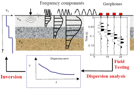
At the shallow depths, the stratum is generally a vertically heterogeneous medium. As a result, the phase velocity of surface wave propagating in the medium is a function of frequency, a phenomenon is called dispersion. The dispersion of the phase velocity of surface wave is governed by the mechanical properties of the layered medium. Once the phase velocity as a function of frequency is obtained, the mechanical properties of the medium can be inversely determined. Following this concept, Surface wave methods generally involve three major steps: (1) Generating artificial perturbations on tested sites and recording the seismograms via receivers (Geophones) and a seismograph. (2) Determination of the experimental dispersion curve by signal processing procedures from the collected field seismograms. (3) Determination of the stiffness profile from the experimental dispersion curve by an inversion algorithm.
Comparing with SSRW and SASW, MASW has advantages of field efficiency, automatic analysis, and data redundancy. Despite its advantages over conventional SSRW and SASW, the testing configuration remains a crucial factor that may affect the test results. To avoid errors and ambiguities caused by physical phenomena and digital signal processing, some constraints on survey line configurations diminish the convenience and feasibility of MASW.
Tradeoffs are involved when selecting the testing parameters. Especially for inexperienced testers, it could be a perplexity when conducting tests in the field. Furthermore, several algorithms with different preference in the literature exit for the dispersion analysis. A standard and preferred guideline is yet to be proposed for engineering practice.
1.2 Objectives
The wavefield recorded in-situ directly decides the quality of the result. The raw data is a time-space discretized wavefield and influenced by wave propagation phenomena and discrete recording. The dispersion curve analysis from the recorded data is affected by higher modes of wave propagation and discretization and truncation of wavefield. An inadequate testing configuration might cause deficient results for specific engineering problems. Although some rules are available for selecting the testing parameters, tradeoffs are involved and no clear guideline is available for conducting MASW tests.
Several algorithms were proposed to analyze the dispersion relations from the recorded wavefield. The analysis usually starts with a transformation from the original time-space (t-x) domain to the frequency-space (f-x) domain. The SASW uses only the information of phase angle verse offsets. It usually requires careful manual attention and is quite time-consuming due to the associated phase angle unwrapping (Lin et al, 2002). Other methods of dispersion analysis involve another sequential transformation. They transform the survey data in t-x domain into frequency- wavenumeber (f-k) (Capon, 1969; Yilmaz, 1987; Alleyne et al, 1990; Forchap et al, 1998; Lu et al, 2004), frequency- slowness (f-p) (McMechan et al, 1981) or frequency- velocity (f-v) (Park et al, 1998b) domains. Whether the dispersion relation in f-k,
f-p and f-v spectra can be clearly and accurately identified depends not only on the complexity
of strata and field configuration, but also on the discrete transformation algorithms. Several studies have made comparisons among aforementioned transformation algorithms, but
different algorithms were favored without consensus (Foti, 2000; Beaty, 2002; O’Neil, 2004; Mora, 2003; Xia et al, 2005).
Lack of standard guidelines for choosing the testing configuration and performing the dispersion analysis, the MASW method becomes ambiguous and the degree of success of MASW testing is uncertain. Incorrect results may occur, not from the inherent limitations of MASW, but due to negligence or mistakes from experimenters’ lacks of expertise and experience. Therefore, this study is aimed to propose some operation principles or standard procedures for eliminating or mitigating those unnecessary errors and uncertainties. Besides ensuring the correctness, the proposed procedure is intended to optimize the investigation depth and resolution.
1.3 Dissertation outline
This study mainly focuses on field testing and dispersion analysis of MASW. It attempts to explicitly establish a set of standard procedures and logical thinking as guidelines for MASW experimenters. There are three major divisions of this dissertation. The motivation, objectives, and fundamental background of this study are introduced in the first part. The second part studies the effects on the field parameters and standardization of field testing. The last part is related to the unification of algorithms and techniques for enhancing the resolution and correctness of dispersion analysis.
The presentation of background in Chapter 2 includes several aspects. The dynamic properties of soil, laboratory and in-situ testing methods are first introduced. The basic theory of wave propagation and computation of dispersion curve and synthetic wavefield of surface wave will then follow. The last part gives an overall review on seismic tests using surface wave with emphasis on the field testing, dispersion analysis and inversion of MASW.
MASW. Although the corresponding rule for each temporal or spatial parameter can be made, the interworking of spatial parameters leads to conflict or dilemma. An innovative testing procedure and the associated signal processing is proposed to resolve the dilemma and standardize the testing procedure, which can also be used to optimize investigation depth and the lateral resolution. In addition, seismic sources for greater energy and lower frequency and sensors for better testing convenience are suggested and applied in this study.
Chapter 4 proposes a unified approach for dispersion analysis. The procedure starts with a method called multi-channel spectral analysis of surface wave (MSASW). It provides not only a preliminary dispersion analysis but also evaluation of data quality and optimum offset selection for removing the near and far field effects. The procedure is followed by the unified algorithm that transforms the time-space wavefield into f-k, f-p, f-v and f-λ domains simultaneously. The dispersion curves obtained by different transformation are shown to be equivalent by a newly-proposed optimization method for dispersion analysis. Further investigations on the data sampling of the dispersion curve are also discussed in this chapter.
Finally some conclusions and suggestions are summarized in Chapter 5. A set of operation principles or standard procedures of field testing and dispersion analysis of MASW is clearly proposed for experimenters. Future researches are also suggested in the end.
2 Literature review
2.1 Dynamic properties of soil and testing methods
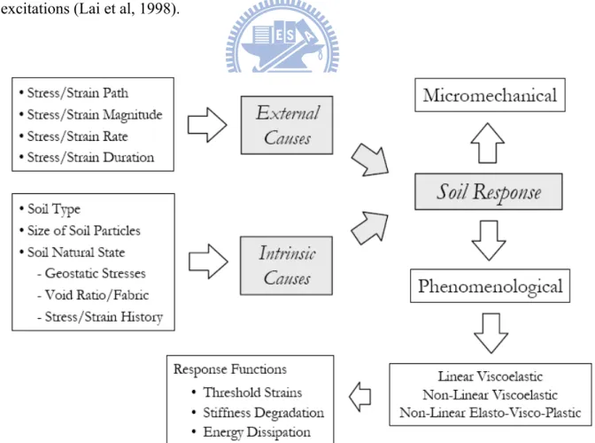
2.1.1 Dynamic properties of soilVariables and factors affecting the dynamic behavior of a soil according to the previous can be broadly divided into two categories according to their origin: external variables and intrinsic variables. The external variables include the stress/strain path, stress/strain magnitude, stress/ strain rate, stress/strain duration and so on; the intrinsic variables include the soil type, the size of soil particles and the state parameters. The state parameters include the effective stress, the arrangement of soil particles and the stress-strain history. Fig. 2-1 summarizes the relationships between causes and effects in the response of soils to dynamic excitations (Lai et al, 1998).
Fig. 2-1 Cause-effect relationships in soil response to dynamic excitations (Lai et al, 1998)
Experimental evidence also shows that the magnitude of the applied stress or strain is the most important factor among the external variables affecting soil responses to dynamic excitations (Lai et al, 1998). Some important features of soil behaviors are reported for the different intervals of cyclic shear strains. Based on these findings, it was then possible to define a shear strain spectrum for simple shear conditions where distinct types of soil behaviors were identified (EPRI, 1991; Vucetic, 1994).
A threshold shear strain called linear cyclic threshold shear strain (Vucetic, 1994), γtl, is
defined for the very small stain region, 0<γ<γtl. In this region the soil behaves linearly
(without stiffness degradation) but not elastically (with energy dissipation) (Kramer, 1996). The value of γtl varies considerably with the soil type. For example, γtl for sands is on the order of 10-3%, whereas for normally consolidated clays with a plasticity index (PI) of 50, γtl is on the order of 10-2% (Lo Presti, 1987; Lo Presti, 1989).
The small strain region is defined as γtl<γ<γtv, in which γtv is called volumetric
threshold shear strain (Vucetic, 1994). Once γ exceeds γtv, there are irrecoverable volumetric
change in drained tests and increases of pore-water pressure in undrained tests (Vucetic, 1994). In this region soil behaviors is non-linear and inelastic but material properties do not change rapidly and degrade little with increasing shear strain and number of loading cycles increasing (Lai et al, 1998). The values of γtv are on the order of 10-3% for gravels, 10-2% for sands, and
10-1
% for normally consolidated, high plasticity clays (Bellotti et al, 1989;Lo Presti, 1989;Vucetic et al, 1991).
The intermediate strain region is defined as γtv<γ<γtpf, in which γtpf is called pre-failure threshold shear strain (Vucetic, 1994). Due to irrecoverable volumetric changes in the previous stage, both instantaneous energy dissipation and losses occur as the number of loading cycles increases (Vucetic, 1994). In this range of deformation the degradation of soil properties with the shear strain is apparent not only within the hysteretic loop but also with
the increase of number of cycles (Ishihara, 1996).
The last region is defined as γtpf<γ<γtf for large strains (EPRI, 1991;Vucetic, 1994). In the region soil behaviors is highly non-linear and inelastic preceding the condition of failure occurring at the failure threshold shear strain γtf.
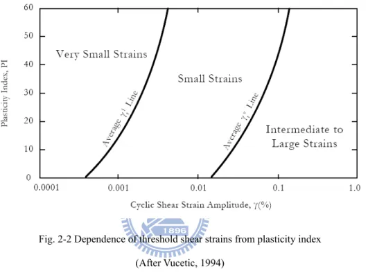
Fig. 2-2 Dependence of threshold shear strains from plasticity index (After Vucetic, 1994)
Among the threshold strains mentioned above, the γtl and γtv are particularly important.
Because γtl separates the linear (though inelastic) responses from the non-linear responses of
soil under cyclic excitation. The magnitude of these two threshold shear strains strongly depends on the plasticity of soil. Fig. 2-2 shows the dependence of threshold shear strains on
plasticity index (Vucetic, 1994). The γtv distinguishes different types of irrecoverable
deformations occurring in soils undergoing harmonic oscillations. These changes result in two observable effects: stiffness reduction and entropy density production (Lai et al, 1998).
Soils show nonlinear variation in shear modulus with shearing strain (G –log γ curve) and in shear stress with shearing strain (τ –γ curve). However, in addition to dynamic response, the importance of small-strain stiffness on static deformation analysis has also been pointed out,
especially for analyses of settlement and soil structure interaction. Furthermore, Stokoe et al. (2004) show that Vs measurement in the field is a critical component in evaluating sample disturbance and in predicting nonlinear G – log γ and τ – γ curves. A few successful demonstrations of the use of seismically determined soil modulus for settlement predictions have been presented (see, for example, Shibuya et al. 1994, Jardine et al. 1998, Jamiolkowski et al. 2001, Di Benedetto et al. 2003, and Stokoe et al. 2004).
2.1.2 Testing methods
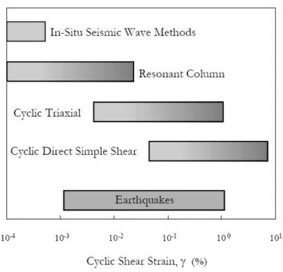
There are many techniques available in-situ or in laboratory for measurement of dynamic soil properties. Each of them has its own advantages and limitations with respect to different engineering problems. As mentioned above, soil behaviors under dynamic loading are mainly affected by the magnitude of shear strains. The Fig. 2-3 shows the ranges of shear strain amplitude of some laboratory and in-situ tests compared to those induced by earthquakes. A broad introduction on laboratory and in-situ tests will be present in the following sections in which tests are categorized by induced strain levels.
Fig. 2-3 Ranges of variability of cyclic shear strain amplitude in laboratory and in-situ tests (Ishihara, 1996)
Under a well-controlled circumstance, laboratory tests definitely have advantages on precise measurement, repeatability and controlled boundary condition. However, original conditions of soil are usually altered during sampling tasks and it may be difficult for some kinds of soil to be sampled. Laboratory tests on samples are also time consuming and cost effective.
The main advantage of in-situ tests is no need for sampling. This avoids degrees of disturbance of soil specimen brought by sampling. Another nice feature of in-situ tests is more spatially representative since in-situ tests measure the responses of a relatively large volume of soil. Furthermore many in-situ tests induce the deformations similar to problems of interest, especially seismic tests. However, for most of in-situ tests, field operations lack of standard procedures and data interpretation is generally more difficult. That makes in-situ tests not user friendly. The comparison between in-situ and laboratory tests is summarized on Table 2.1.
Table 2.1 Measurement of low-Strain dynamic properties of soils comparison between in-situ and laboratory techniques
(Lai et al, 1998)
2.1.2.1 Laboratory tests
For laboratory tests, as shown in Table 2.2, only few of them provide ability to measure the soil dynamic properties at low strain levels. At high-strain level, the volume of soil usually has irrecoverable change. Under drained condition it is easily to be observed from changes in volumetric strain. When under undrained condition the tendency of volume change in volume results in the change in porewater pressure and effective stress. So methods in this category should have capability to control the porewater drainage and measure the change in volume and stress.
Table 2.2 Laboratory tests for measuring dynamic properties of soil
Test strain
level Note
Resonant column test Low
1. Most common used in laboartory 2. Well control testing condition
3. Both stiffness and damping of soil measured Ultrasonic pulse test and Piezo-
electric bender element test
Low
1. Useful for very soft materials
2. Incorporated into conventional cubical txiaxial devices and other
Cyclic triaxial test
Cyclic direct simple shear test Cyclic torsional shear test
High
1. Most commonly used at high strain levels
2. Control the porewater drainage and measure the change in volume and stress
2.1.2.2 Field tests
Field tests for measuring dynamic properties of soil, as shown in Table 2.3, induce different levels of strain. When selecting an appropriate test for purposes, the representatives of the soil behaviors shall be considered. Another important concern is the necessity of invasive tasks. Some of the tests need drilling of boreholes or penetration of testing devices, while some can be performed on the ground surface non-destructively. Tests performed on the ground surface are usually more efficient and cost effective. They are practically useful for geomaterials in which drilling and penetration are difficult. But the information gained from borehole tests is more direct than tests on ground surface.
Most of the high-strain tests aim to measure characteristics like soil strength at high-strain level and can be correlated to the low-strain behaviors. Several high-strain tests are common used in geotechnical engineering of different purposes. Basically the strains induced by low-strain tests are usually small enough for assuming linear stress- strain behavior of soil, in other words, the strain is smaller than the linear cyclic threshold shear
strain γtl. Most of them are based on the theory of wave propagation in linear materials. The
measured body or surface wave velocity and frequencies or wavelengths can all be directly related to the low-strain mechanic modulus of a soil.
Seismic tests involve generating a transient or steady stress wave and interpreting soil dynamic properties via measurements made at one or more different locations. Stress waves may be generated by various seismic sources ranging from sledgehammers to buried explosive charges. The measurement can be the distance and traveling time of waves or a digitized wavefield recorded by array receivers. For those needing boreholes, results (mostly wave velocities verse depth profile) can be easily obtained from simple computation of traveling time and distance of wave. But for those performed on the ground surface, the characteristic properties (such as traveling time- distance relation, dispersion relation) involve the signal processing of raw data (recorded digitized wavefield) and final results need inversion based on certain theories and hypothesis. The more complicated the interpretation process, the more uncertainty of results and expertise of testers required.
Non-invasive methods for measuring shear wave velocity include shear wave refraction survey and surface wave methods. Refraction techniques for near surface survey are traditionally based on head-wave methods. Recent developments in refraction tomography have enhanced the spatial resolution of the refraction survey. However, the results are subject to limitation that velocity must increase with depth. Furthermore, S-wave refraction survey may not provide the true S-wave velocity because of wave-type conversion in an area of non-horizontal layers. Surface wave methods do not suffer from aforementioned problems associated with refraction survey, hence are considered of special interest for the site surveys of geotechnical problems.
Table 2.3 Field tests for measuring dynamic properties of soil
Test strain
level
Borehole
required Remarks
Seismic reflection test Low No
Reflected signals are recorded typically using common midpoint arrays. Velocity between reflectors may be estimated during normal move out correction.
Seismic refraction test Low No
Velocity profile is deduced from recording the first arrival times versus source-to-receiver dstance.
Seismic tests using surface wave Low No
Steady State Rayleigh Wave method (SSRW) Spectral Analysis of Surface Waves Method (SASW)
Multi-station Analysis of Surface Waves method (MASW)
Suspension logging test Low Yes
Frequency components are much higher than those of interest in geotechnical earthquake engineering
Seismic cross-hole test Low Yes At least two boreholes required Seismic down-hole (up-hole) test Low Yes Only one borehole required Standard Penetration Test (SPT)
Cone Penetration Test (CPT) Dilatometer Test (DMT) Pressuremeter Test (PMT)
2.2 Wave propagation and computation of surface wave
There are various kinds of wave produced when an impulse was applied on the ground surface. These waves generally are categorized into two main types: body waves and surface waves. Body waves travel through the interior of the medium. Surface waves are the result of the interaction between body waves, the free surface and surficial layers of the medium. They travel along the surface with amplitudes decreasing roughly exponentially with depth.
Body waves are of two types: P wave and S wave. P wave is also referred to as primary, compressional or longitudinal wave consisting of successive compression and relaxation of the medium. The individual particle moves parallel to the direction of P wave propagation. S wave is also known as secondary, shear or transverse wave. It induces the shearing deformation as it traveling through the medium. The particle motion when S wave traveling is perpendicular to the direction of S wave propagation. For a three dimensional coordination, the S wave has two components: the movement on vertical plane is SV wave and the movement on horizontal plane is SH wave. The velocities of body wave propagation depend on the stiffness of medium.
The surface waves include are Rayleigh wave and Love wave. Rayleigh wave generated by interaction of P wave and SV wave involves both vertical and horizontal particle motions. Love wave is produced by the interaction of SH wave with a surficial soft layer and it has no vertical particle motion. There is no Love wave on the surface in a half space without any interface of layers. The basic theory of elastic wave propagation and the characteristics of Rayleigh wave, the main role of this study, will be introduced in the following paragraphs.
2.2.1 Basic theory of elastic wave propagation 2.2.1.1 Stress, strain and their relationship
¾ Definition and notation of stress
Fig. 2-4 Stress notation of an element in an x-y-z Cartesian coordination
σij is usually used as the symbol representing stress. In the subscript, the first letter
denotes the axis perpendicular to the plane in which the stress acts and the second denotes the direction of stress. For a small element in an x-y-z Cartesian coordination, there are totally nine components acting on its face (as shown on Fig. 2-4).
The normal stresses are denoted as: σxx , σyy , σzz
The shear stresses are denoted as: σxy , σxz , σyx , σyz , σzx , σzy
For the moment equilibrium of the element, it requires that σxy =σyx , σxz =σzx , σyz =σzy. So there are only six independent components required for describing the state of stresses of an element.
¾ Definition and notation of displacement and strain
Let ui represent the displacement in i direction. The relationship between displacements
and strains can be defined as: ⎟⎟ ⎠ ⎞ ⎜⎜ ⎝ ⎛ ∂ ∂ + ∂ ∂ = i u j ui j ij 2 1 ε (2-1) For example, ⎟ ⎠ ⎞ ⎜ ⎝ ⎛ ∂ ∂ + ∂ ∂ = ⎟⎟ ⎠ ⎞ ⎜⎜ ⎝ ⎛ ∂ ∂ + ∂ ∂ = ∂ ∂ = ⎟ ⎠ ⎞ ⎜ ⎝ ⎛ ∂ ∂ + ∂ ∂ = x u z u x u y u x u x u x u z x xz y x xy x x x xx 2 1 2 1 2 1 ε ε ε (2-2) ¾ Stress-strain relationship
For a homogeneous and isotropic linear elastic body, the stress-strain constitutive law can be described by two Lame’s constants, λ and μ, and Hooke’s law. The generalized form can be writen as:
ij ij
kk
ij λε δ με
σ = +2 (2-3)
where the volumetric strain εkk=εxx +εyy +εzz and δij represents Kronecker delta
function. For example, substituting (2-2) into (2-3) gives
⎟ ⎠ ⎞ ⎜ ⎝ ⎛ ∂ ∂ + ∂ ∂ = ⎟⎟ ⎠ ⎞ ⎜⎜ ⎝ ⎛ ∂ ∂ + ∂ ∂ = ∂ ∂ + ⎟⎟ ⎠ ⎞ ⎜⎜ ⎝ ⎛ ∂ ∂ + ∂ ∂ + ∂ ∂ = x u z u x u y u x u z u y u x u z x xz y x xy x z y x xx μ σ μ σ μ λ σ 2 (2-4)
Consider the infinitesimal element shown on Fig. 2-4 with dimensions of dx, dy and dz respectively in x, y and z direction. In the x direction, the unbalanced external force must be balanced by an inertial force in that direction. So,
(
)
x zx zx zx yx yx yx xx xx xx x f dxdy dxdy dz z dxdz dxdz dy y dydz dydz dx x t u dxdydz + − ⎟ ⎠ ⎞ ⎜ ⎝ ⎛ ∂ ∂ + + − ⎟⎟ ⎠ ⎞ ⎜⎜ ⎝ ⎛ ∂ ∂ + + − ⎟ ⎠ ⎞ ⎜ ⎝ ⎛ ∂ ∂ + = ∂ ∂ σ σ σ σ σ σ σ σ σ ρ 22 (2-5)in which ρ is density and fi is the body force in i direction. Supposing fi = 0, repeating the operation in y and z directions gives
z y x t u z y x t u z y x t u zz yz xz z zy yy xy y zx yx xx x ∂ ∂ + ∂ ∂ + ∂ ∂ = ∂ ∂ ∂ ∂ + ∂ ∂ + ∂ ∂ = ∂ ∂ ∂ ∂ + ∂ ∂ + ∂ ∂ = ∂ ∂ σ σ σ ρ σ σ σ ρ σ σ σ ρ 2 2 2 2 2 2 (2-6)
(2-6) represent the three dimensional equations of motion of solid. The equations are derived on the basis of equilibrium, therefore it is valid for solids of any constitutive model. Substituting (2-4) derived from Hooke’s law into the equations of motion and repeating the operation in y and z directions, the equations of motion expressed in term of displacement are shown as following: ⎟⎟ ⎠ ⎞ ⎜⎜ ⎝ ⎛ ∂ ∂ + ∂ ∂ + ∂ ∂ + ⎟⎟ ⎠ ⎞ ⎜⎜ ⎝ ⎛ ∂ ∂ + ∂ ∂ + ∂ ∂ ∂ ∂ + = ∂ ∂ ⎟ ⎟ ⎠ ⎞ ⎜ ⎜ ⎝ ⎛ ∂ ∂ + ∂ ∂ + ∂ ∂ + ⎟⎟ ⎠ ⎞ ⎜⎜ ⎝ ⎛ ∂ ∂ + ∂ ∂ + ∂ ∂ ∂ ∂ + = ∂ ∂ ⎟⎟ ⎠ ⎞ ⎜⎜ ⎝ ⎛ ∂ ∂ + ∂ ∂ + ∂ ∂ + ⎟⎟ ⎠ ⎞ ⎜⎜ ⎝ ⎛ ∂ ∂ + ∂ ∂ + ∂ ∂ ∂ ∂ + = ∂ ∂ 2 2 2 2 2 2 2 2 2 2 2 2 2 2 2 2 2 2 2 2 2 2 2 2 ) ( ) ( ) ( z u y u x u z u y u x u z t u z u y u x u z u y u x u y t u z u y u x u z u y u x u x t u z z z z y x z y y y z y x y x x x z y x x μ μ λ ρ μ μ λ ρ μ μ λ ρ (2-7)
u u u•=( + )∇(∇⋅ )+ ∇2 • μ μ λ ρ (2-8)
in which, overdots are used to indicate time derivatives (e.g., u• =∂u ∂t, •u•=∂2u ∂t2), ∇ 2
represents the Laplacian operator. The Laplacian operator has another alternative expression: ) ( ) ( 2u=∇ ∇⋅u − ∇×∇×u ∇ (2-9)
Then (2-8) can be written as following: ) ( ) ( ) 2 ( u u u•= + ∇ ∇⋅ − ∇×∇× • μ μ λ ρ (2-10)
According to the Helmholtz decomposition theorem, any vector field u can be considered to be generated by a pair of potentials: a scalar potential ψ and a vector potential Ψ.
Ψ × ∇ + ∇ = φ u (2-11) in which, 0 , 0 ∇⋅Ψ = = × ∇ φ (2-12)
Substituting (2-11) into (2-10) gives, 0 ) 2 ( 2 2 = ⎥⎦ ⎤ ⎢⎣ ⎡ ∇ − × ∇ + ⎥⎦ ⎤ ⎢⎣ ⎡ + ∇ − ∇ λ μ φ ρ•φ• μ ψ ρψ•• (2-13) let ρ μ ρ μ λ = + = s p v v 2 , (2-14)
Substituting (2-14) into (2-13), then (2-13) has solutions if the (2-15) are satisfied. 0 1 , 0 1 2 2 2 2 − = ∇ − = ∇ φ φ•• ψ ψ•• s p v v (2-15)
(2-15) are the wave equations, in which vP and vS are the propagating velocities of P
wave and S wave respectively. As it shown, the displacements of solid after disturbance can be categorized into those related to P wave and those related to S wave. The propagating velocities of body waves in a solid are not correlative with the frequency of excitation but
correlative only with the Lame’s constants of the medium. From (2-14), it is obvious that vP is
greater than vS. It can be observed on the seismogram of earthquake that the displacements
caused by P wave always occur earlier than those caused by S wave.
The separation of variables is applied here for solution of wave equations (2-15). Suppose ) ( ) ( ) ( ) ( ) , , , (x y z t = X x Y y Z z T t φ (2-16)
Substituting (2-16) into (2-15), the general solution of the wave scalar potential for plane waves propagating in any direction is obtained,
(
)
[
i t k x k y k z]
A t z y x, , , ) exp px2 py2 pz2 ( = ± ω ± ± ± φ (2-17) in which, p pz py px v k k k 2 + 2 + 2 =ω2 (2-18)(2-18) defines the surface of plane waves propagating in directions of (kpx, kpy, kpz) with a P
wave velocity of vp in a Cartesian coordinate. The constant A represents the amplitude. In the
same way, the general solution of the wave vector potential for plane waves propagating in any direction can be obtained.
(
)
[
i t k x k y k z]
B t z y x, , , ) exp sx2 sy2 sz2 ( = ± ± ± ± Ψ ω (2-19) in which, s sz sy sx k k v k 2+ 2+ 2 =ω2 (2-20)(2-19) defines the surface of plane waves propagating in directions of (ksx, ksy, ksz) with an S wave velocity of vs in a Cartesian coordinate. The constant B represents the amplitude.
Base on the hypothesis of no inference when P and S wave propagating, the displacement field u caused by excitation can be represented by the linear combination of the vibrations caused by P wave and S wave. According to the Helmholtz theorem, the
displacement field u can be decomposed into: Ψ × ∇ + ∇ = + =up us φ u (2-21)
in which up, us represent the displacement caused by P wave and S wave respectively. So,
∧ ∧ ∧ ∧ ∧ ∧ ⎟⎟ ⎠ ⎞ ⎜⎜ ⎝ ⎛ ∂ Ψ ∂ − ∂ Ψ ∂ + ⎟ ⎠ ⎞ ⎜ ⎝ ⎛ ∂ Ψ ∂ − ∂ Ψ ∂ + ⎟⎟ ⎠ ⎞ ⎜⎜ ⎝ ⎛ ∂ Ψ ∂ − ∂ Ψ ∂ = Ψ × ∇ = ∂ ∂ + ∂ ∂ + ∂ ∂ = ∇ = z y x y x z x z y u z z y y x x u x y z x y z s p φ φ φ φ (2-22)
in which, Ψx, Ψy , Ψz represent the components of Ψ in x, y, z directions. Equation (2-22)
also satisfies the form of general solution as shown in (2-19). ∧x ,,∧y ∧z represent the unit vectors in x, y, z directions. For simplifying the problem, the plane wave is supposed that kpy,
ksy =0, which means the wave is steady in y direction, ∂φ ∂y→0 and ∂Ψi ∂y→0. Then us can be expressed as:
∧ ∧ ∧ ∧ ∧ ⎟⎟ ⎠ ⎞ ⎜⎜ ⎝ ⎛ ∂ Ψ ∂ + ⎟ ⎠ ⎞ ⎜ ⎝ ⎛ ∂ Ψ ∂ − ∂ Ψ ∂ + ⎟⎟ ⎠ ⎞ ⎜⎜ ⎝ ⎛ ∂ Ψ ∂ − = ∂ ∂ + ∂ ∂ = z x y x z x z u z z x x u y z x y s p φ φ (2-23)
The equation (2-21) can be re-written by substituting (2-22) and (2-23).
∧ ∧ ∧ ⎟⎟ ⎠ ⎞ ⎜⎜ ⎝ ⎛ ∂ Ψ ∂ + ∂ ∂ + ⎟ ⎠ ⎞ ⎜ ⎝ ⎛ ∂ Ψ ∂ − ∂ Ψ ∂ + ⎟⎟ ⎠ ⎞ ⎜⎜ ⎝ ⎛ ∂ Ψ ∂ − ∂ ∂ = z x z y x z x z x u φ y x z φ y (2-24)
From the result of (2-24), the displacement in y direction depends only on S wave. But
displacements in x and z direction is a combination provided by P wave and S wave and the
interference of S wave here is different from the interference of S wave in y direction.
Distinctly, the displacement field u can be discussed separately in the x-z plane and y direction.
The displacement in y direction is represented by SH wave and the displacement in x-z plane
2.2.1.3 Rayleigh wave in a homogeneous halfspace
A free surface is necessary for occurrence of surface waves. The main characteristic of surface waves is that the carried energy decays with increasing depth. Surface wave in a homogeneous halfspace is the focus of this section. From (2-24), it is clear that the components of the displacement field u in x, y, z directions are:
x z u x z u z x u y z z x y y x ∂ Ψ ∂ + ∂ ∂ = ∂ Ψ ∂ − ∂ Ψ ∂ = ∂ Ψ ∂ − ∂ ∂ = φ φ (2-25)
As mentioned above, the uy depends only on the vector potential of S wave. Keeping it in
term of uy does not affect the form of general solution. For a wave with a frequency of ω and
velocity of vR traveling through a homogeneous halfspace, its φ, Ψy and uy can be supposed as:
(
)
[
]
(
)
[
]
(
)
[
ik x v t]
z h u t v x ik z g t v x ik z f R y R y R − = − = Ψ − = exp ) ( exp ) ( exp ) ( φ (2-26)in which, f(z), g(z), h(z) are used for the phenomenon that energy decays gradually with depth
(z) increasing; k=w/ vR represents spatial frequency. Putting (2-26) into (2-15) leads to
0 ) ( ) ( " 0 ) ( ) ( " 0 ) ( ) ( " 2 2 2 2 2 2 = + = + = + z h s k z h z g s k z g z f r k z f (2-27) in which 2 / 1 2 2 R 2 / 1 2 2 R 1 v 1 v ⎟⎟ ⎠ ⎞ ⎜⎜ ⎝ ⎛ − = ⎟ ⎟ ⎠ ⎞ ⎜ ⎜ ⎝ ⎛ − = s p v s v r (2-28)
( )
(
)
( )
(
)
( )
iksz C(
iksz)
C z h iksz B iksz B z g ikrz A ikrz A z f − + = − + = − + = exp exp ' ) ( exp exp ' ) ( exp exp ' ) ( (2-29)in which, A, A’, B, B’, C, C’ are all arbitrary constants. The constants A’, B’, C’ equal to zero due to the behavior of energy decay with depth increasing. Both of r and s are imaginary numbers, which implies vp> vs> vR. Substituting (2-29) into (2-26) gives,
(
)
[
]
(
)
[
]
(
)
[
ikrz ik x v t]
C u t v x ik ikrz B t v x ik ikrz A R y R y R − + − = − + − = Ψ − + − = exp exp exp φ (2-30)The boundary conditions are necessary for resolving the constants A, B, C. On the free
surface, the stresses in z direction must be zero, σzz =0, σzx =0, σzy =0. The boundary
conditions here are:
0 0 0 2 = ⎟⎟ ⎠ ⎞ ⎜⎜ ⎝ ⎛ ∂ ∂ + ∂ ∂ = = ⎟ ⎠ ⎞ ⎜ ⎝ ⎛ ∂ ∂ + ∂ ∂ = = ∂ ∂ + ⎟⎟ ⎠ ⎞ ⎜⎜ ⎝ ⎛ ∂ ∂ + ∂ ∂ + ∂ ∂ = z u y u z u x u z u z u y u x u y z zy x z zx z z y x zz μ σ μ σ μ λ σ (2-31)
Substituting (2-24) and (2-29) into (2-31), that gives:
(
2)
2 0 0 0 2 2 2 2 2 2 2 2 2 2 = ∂ ∂ Ψ ∂ + ∂ ∂ + ∂ ∂ ∂ + = ∂ ∂ = ∂ Ψ ∂ − ∂ Ψ ∂ + ∂ ∂ ∂ x z x x z z u y x x z y y y y μ φ λ φ μ λ φ (2-32)Substituting the third of (2-30) into the second of (2-32) resolves that the constant C
equals zero which means no displacement in y direction (uy=0). It implies the surface wave in
a homogeneous halfspace does not contain Love wave. Next, substituting the first and the second of (2-30) into the first and third of (2-32) respectively obtains a homogeneous system
of linear equations.
(
)
[
1 2]
2 0 0 ) 1 ( 2 2 2 2 = − − + = − − sB v A v r v B S rA s s p (2-33)If nontrivial solutions of (2-33) exist, the following requirement should be satisfied,
(
)
0 2 2 1 ) 1 ( 2 2 2 2 = − − + − − s v v r v s r s s p (2-34)Calculating the determinant gives
(
)
[
2 +1 −2]
(1− 2)−4 2 =0 s s p r v s rsv v (2-35)Substituting (2-28) into (2-35) and rearranging,
2 / 1 2 2 2 / 1 2 2 2 2 2 1 1 4 2 ⎟⎟ ⎠ ⎞ ⎜⎜ ⎝ ⎛ − ⎟⎟ ⎠ ⎞ ⎜⎜ ⎝ ⎛ − = ⎟⎟ ⎠ ⎞ ⎜⎜ ⎝ ⎛ − s R P R s R v v v v v v (2-36)
(2-36) is first presented by Rayleigh in 1887 for the wave velocity of Rayleigh wave. The equation clearly shows that the propagating velocity of Rayleigh wave in a homogeneous halfspace is irrelevant to frequency (which means non-dispersive).
Let P s s R v v q v v = = , ξ (2-37)
Substituting (2-37) into (2-36) and rearranging,
(
3 2)
16( 1) 0 88 2
3− ξ + − qξ+ q− =
ξ (2-38)
in which, q is a constant once the Lame’s constants of the homogeneous halfspace are assured. ξ is the only unknown which have three nontrivial solutions for the cubic equation. The propagating velocity of Rayleigh wave, vR, wave should satisfy the requirement of vp > vs > vR. Therefore the solution satisfyingξ<1 is the one for the propagating velocity of Rayleigh wave.
typical values of Poisson’s ratio, 0.2<ν<0.4, the velocity of Rayleigh wave ranges from 0.9
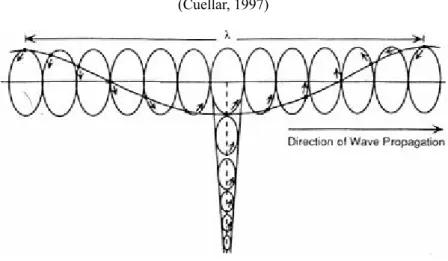
vs to 0.95 vs. The ratios between vR, vp and vs as a function ofνis shown in Fig. 2-5. The particle motion of a propagating Rayleigh wave in a homogeneous half space transits from retrograde to prograde elliptical with depth as shown in Fig. 2-6 and Fig. 2-7. The Rayleigh wave comprises both compressional and rotational components and the eccentricity of the ellipse for locus of particle motion depends on Poisson’s ratio.
Fig. 2-5 The ratio of Rayleigh wave velocity, vR, verse body wave velocities as a function of Poisson ratio,ν
(Sheriff et al, 1982)
Fig. 2-6 Rayleigh wave particle motion in a homogeneous, isotropic half space; retrograde at the surface, passing through purely vertical at about λ/5 then becoming prograde at depth
(Cuellar, 1997)
Fig. 2-7 Particle motions of Rayleigh wave over one wavelength along the surface and as a function of depth (Sheriff et al, 1982)
2.2.1.4 Rayleigh wave in a vertically heterogeneous halfspace
The surface wave applied in this study is Rayleigh wave due to the interference of P wave and SV wave. Its most important characteristic is dispersion due to the stiffness variation with depth of the tested strata. Dispersion means the propagating velocity of wave varies with frequency.
Considering a vertically heterogeneous halfspace as shown in Fig. 2-8, the elastic parameters depend only on the depth z. The following discussion focuses only on the part
related to P-SV wave, so the component of displacement on y direction, uy, is assumed to be
zero. For a plane wave propagating in +x direction, it can be expressed as:
(
)
[
(
)
]
(
k z)
[
i(
kx t)
]
ir u t kx i z k r u z x ω ω ω ω − = − = exp , , exp , , 2 1 (2-39)in which, r1(k,z,ω) and r2 (k,z,ω) represent the amplitudes of components of the displacement in x and z directions respectively. Both have characteristics of decay with z increasing and each different frequencyωwith a corresponding spatial frequency k.
Due to the continuity of stress between layers, so let
(
)
[
(
)
]
(
k z)
[
i(
kx t)
]
ir t kx i z k r zz zx ω ω σ ω ω σ − = − = exp , , exp , , 4 3 (2-40)in which, r3 (k,z,ω) and r4 (k,z,ω) represent the amplitudes of stresses on plane z in x and z directions respectively. Both have characteristics of decay with z increasing and each different frequencyωwith a corresponding spatial frequency k.
For solutions of r1 (k,z,ω), r2 (k,z,ω), r3 (k,z,ω) and r4 (k,z,ω), it is necessary to obtain four equations for four unknowns. Two can be obtained from the stress-strain relationship,
( )
( )
( )
⎟ ⎠ ⎞ ⎜ ⎝ ⎛ ∂ ∂ + ∂ ∂ = ∂ ∂ + ⎟ ⎠ ⎞ ⎜ ⎝ ⎛ ∂ ∂ + ∂ ∂ = z u x u z z u z z u x u z x z zx z z x zz μ σ μ λ σ 2 (2-41)Substituting (2-39) into (2-41) gives
( )
( )
(
)
[
(
)
]
( )
[
(
)
]
( )
[
(
)
]
[
(
)
]
⎟ ⎠ ⎞ ⎜ ⎝ ⎛− − + − = − + − + = t kx i dz dr t kx i kr z t kx i kr z i t kx i dz dr z z i zx zz ω ω μ σ ω λ ω μ λ σ exp exp exp exp 2 1 2 1 2 (2-42)( )
( )
( )
[
4( )
1]
2 2 3 1 2 1 1 kr z r z z dz dr kr r z dz dr λ μ λ μ − + = + = (2-43)(2-43) are two of four equations for solutions. The other two can be found by means of the equations of motion (2-7),
( )
( ) ( )
( )
( )
( ) ( )
( )
⎟⎟ ⎠ ⎞ ⎜⎜ ⎝ ⎛ ∂ ∂ + ∂ ∂ + ⎟ ⎠ ⎞ ⎜ ⎝ ⎛ ∂ ∂ + ∂ ∂ ∂ ∂ + = ∂ ∂ ⎟⎟ ⎠ ⎞ ⎜⎜ ⎝ ⎛ ∂ ∂ + ∂ ∂ + ⎟ ⎠ ⎞ ⎜ ⎝ ⎛ ∂ ∂ + ∂ ∂ ∂ ∂ + = ∂ ∂ 2 2 2 2 2 2 2 2 2 2 2 2 ) ( ) ( z u x u z z u x u z z z t u z z u x u z z u x u x z z t u z z z z x z x x z x x μ μ λ ρ μ μ λ ρ (2-44)Substituting (2-39) and (2-43) into (2-44) and rearranging,
( )
( ) ( ) ( )
( )
(
( )
)
( )
( )
( )
( )
2 2 2 3 4 4 1 2 2 3 2 2 4 kr r k v z dz dr r z z z k r z z z z z v z k dz dr R R − − = + + ⎥ ⎦ ⎤ ⎢ ⎣ ⎡ ⎟⎟ ⎠ ⎞ ⎜⎜ ⎝ ⎛ + + − = ρ μ λ λ μ λ μ λ μ ρ (2-45)Combining equations (2-43) and (2-45), the motion-stress vector (Aki et al, 2002) can be formed,
( )
( )
( ) ( )
( )
( )
( )
( )
( ) ( )
( )
( )
( ) ( )
( )
( )
( )
⎥ ⎥ ⎥ ⎥ ⎦ ⎤ ⎢ ⎢ ⎢ ⎢ ⎣ ⎡ ⎥ ⎥ ⎥ ⎥ ⎥ ⎥ ⎥ ⎥ ⎦ ⎤ ⎢ ⎢ ⎢ ⎢ ⎢ ⎢ ⎢ ⎢ ⎣ ⎡ − − + − + + − = ⎥ ⎥ ⎥ ⎥ ⎦ ⎤ ⎢ ⎢ ⎢ ⎢ ⎣ ⎡ 4 3 2 1 2 2 2 4 3 2 1 0 0 2 0 0 2 1 0 0 2 0 1 0 r r r r k z z z z k z k z z z z z z k z k r r r r dz d ω ω ρ λ μ λ ω ω ρ ω ζ μ λ μ λ λ ω μ ω (2-46) in which,( )
( ) ( ) ( )
( )
[
( )
]
z z z z z z μ λ μ λ μ ζ 2 4 + + = (2-47)Let f(z)=[r1 r2 r3 r4]T and a matrix A(z) denoting the 4×4 matrix whose elements are functions of stiffness, wavenumber and frequency. (2-47) can be expressed in the form of vector as,
( )
A( ) ( )
z z dz z d f f = (2-48)2.2.2 Computation of theoretical dispersion curve
(2-48) defines a linear eigenvalue problem with displacement eigenfunctions r1 and r2
and stress eigenfunctions r3 and r4. The boundary conditions with the eigenproblem are:
(
)
(
)
(
)
→ →∞ = = = z as z k z at z k r z k r 0 , , 0 0 , , , 0 , , 4 3 ω ω ω f (2-49)And for the continuity of the stress and displacement fields, at each interface of layers in a vertical heterogeneous medium,
( ) ( )
( )
r z n( )
r z n z r u z r u ⋅ = ⋅ = − + − + , , , , σ σ (2-50)For a give frequency ω, (2-48) has nontrivial solutions existing only for specific
wavenumbers kj=kj(ω). The particular kj are the eigenvalues of the eigenproblem and the
corresponding rj(kj,z,ω) are the eigenfunctions. kj=kj(ω) is known in the implicit form as:
( ) ( ) ( )
[
λ ,μ ,ρ , j,ω]
=0R z z z k
F (2-51)
where FR[*] is a function of Lame’s constants, density, wavenumeber and frequency of
excitation. The relationship FR[*]=0 is called Rayleigh dispersion equation. The relationship
shows that Rayleigh wave possesses the characteristic of dispersion in vertically
heterogeneous halfspace. Each kj and its corresponding rj(kj,z,ω) defines a mode of
propagation and there are M modes of propagation at any given frequency. Due to multiple reflections or refractions of wave in layer interfaces, the different modes of propagation at a given frequency are reasonable and a result of constructive inference occurring among waves.
Two tasks are involved for the solution of Rayleigh eigenvalue problem. The first is the
function). The second is the computation of the roots as a function of frequency, which is to find the Rayleigh eigenvalue kj=kj(ω), as illustrated in Fig. 2-9. Once the roots are obtained, it
is straightforward to compute the Rayleigh eigenfunctions rj(kj,z,ω) for understanding the
depth-dependence of displacement and stress as illustrated in Fig. 2-10.
Fig. 2-9 Rayleigh waves dispersion curves in vertically heterogeneous media (Lai et al, 1998)
Fig. 2-10 Rayleigh displacement eigenfunctions in vertically heterogeneous media (Lai et al, 1998)