多屬性多方法潛伏成長模型及其實證應用

行政院國家科學委員會補助專題研究計畫期中進度報告

多屬性多方法潛伏成長模型及其實證應用

Latent Growth Modeling with MTMM and Its Empirical

Applications

計畫編號：NSC 98-2410-H-009-010-MY2

執行期限：98 年 8 月 1 日至 100 年 7 月 31 日

主持人：丁 承 國立交通大學經營管理研究所

Modeling 期刊，研究進度符合預期。我們示範如何利用SAS PROC CALIS/TCALIS進行

誤差共變結構之配適，並提出一基於卡方差異檢定之有效方法以發掘 level-1 誤差共變 結構，另具體說明如何以 PROC TCALIS 中之 SIMTEST statement 進行誤差穩態檢 定，針對外顯變數與潛伏構念之成長模型，皆提供對應的 SAS 語法。

關鍵詞：多屬性多方法，潛伏成長模型，二階成長模型，誤差共變結構，卡方差異檢定， 穩態

This project consists of two parts. The first part is to develop a general multitrait- multimethod (MTMM) latent growth model. The second part is to apply the model proposed to an empirical study in investor sentiment. The focus of the first part is how to identify the error covariance structure. The task has been completed, with a paper submitted to Structural

Equation Modeling. Using SAS PROC CALIS/TCALIS to fit error covariance structures of

latent growth models (LGM) has been illustrated. A tutorial on the SAS syntax is provided for both manifest variables and latent constructs in LGM. While the second-level error covariance structure is usually specified as unstructured, an effective approach for identifying the first-level error covariance structure based on the sequential chi-square difference test is proposed and demonstrated. Moreover, how to test for stationarity of an error process by using the SIMTEST statement in ROC TCALIS is specifically addressed.

Keywords: multitrait-multimethod (MTMM), latent growth model, second-order growth

二、報告內容

The latent growth model (LGM) plays an important role in repeated-measure analysis over a limited occasions in large sample data (e.g., Meredith & Tisak, 1990; Muthén & Khoo, 1998; Preacher, Wichman, MacCallum, & Briggs, 2008, p.12; Singer & Willett, 2003, p.9). The model can not only characterize intraindividual (within-subject) change over time but also examine interindividual (between-subject) difference by means of a random intercept and random slopes, and is a typical application of the multilevel model (or hierarchical linear model (HLM)). The between-subject errors (representing random effects for the intercept and slopes) and the within-subject errors over time are conventionally referred to as level-2 and level-1 errors, respectively.

LGM is also an application of structural equation modeling (SEM) (e.g., Bauer, 2003; Boolen & Curran, 2006; Curran, 2003; Duncan, Duncan, & Hops, 1996; Mehta & Neal 2005; Meredith & Tisak, 1990; Willet & Sayer, 1994). The structural modeling of multilevel data is a relatively new area of methodological research. SEM and HLM stem from different traditional statistical theory, and each has developed its own terminology and standard ways of framing research questions. However, it has become clear that there exists much overlap between the two methodologies under some circumstances. More specifically, when a two-level data structure arises from the repeated observations of a set of individuals over time (such that time is hierarchically nested within an individual), SEM is analytically equivalent to HLM (e.g., Bauer, 2003; Curran, 2003; MacCallum, Kim, Malarkey, & Kiecolt-Glaser, 1997; Raudenbush, 2001; Rovine & Molenaar, 2000; Willett & Sayer, 1994). Thus, despite the inherent differences between the estimation procedures by SEM and HLM, these two approaches provide analytically identical solutions for LGM. Nevertheless, the measurement model capabilities of SEM possess superiority in examining model fit to the HLM approach. The SEM approach also brings the possibility of modeling of change over time for latent constructs or multivariate data (e.g., Bollen & Curran, 2006, Chap. 7, 8; Chan, 1998; Duncan, Duncan, & Strycker, 2006, Chap. 4; Hancock, Kuo, & Lawrence, 2001; MacCallum, et al., 1997; Rovine & Molenaar, 2000). As a result, SEM has become a more commonly used approach for longitudinal data. Specialized software such as Mplus (Muthén & Muthén, 2007), Mx (Neale, Boker, Xie, & Maes, 2003), AMOS (Arbuckle, 2006), EQS (Bentler & Wu, 2005), Lisrel (Joreslog & Sorbom, 2004), and SAS PROC CALIS (TCALIS in SAS 9.2) (SAS Institute Inc., 2007) are readily available and allow individuals to be measured at unique times, having unequal spacing between assessments.

Since errors within the same subject are often correlated across time (e.g., Preacher et al., 2008, p.63; Sayer & Cumsille, 2001), not modeling autocorrelated errors present in longitudinal data or misspecifying error covariance structure has a substantial impact on the inferences for model parameters (e.g., Ferron, Dailey, & Yi, 2002; Kwok, West, & Green, 2007; Murphy & Pituch, 2009; Sivo, Fan, & Witta, 2005). A variety of processes underlying level-1 errors can be used (e.g., Newsom, 2002; Singer & Willett, 2003, Chap. 7; Wolfinger, 1996). The HLM software (Raudenbush, Bryk, & Congdon, 2005) provides the first-order autoregressive (AR(1)) option. The MIXED procedure in SAS/STAT (SAS Institute Inc., 2007) contains many types of level-1 error processes such as unstructured (UN), compound symmetry (CS), AR(1), first-order autoregressive moving average (ARMA(1,1)), Toeplitz (TOEP), Toeplitz with q bands (TOEP(q)), etc. The processes are either stationary or nonstationary. The most general covariance structure is the so-called unstructured model, indicating that no structure is imposed and covariance estimates are to be determined by the data. However, the use of UN is likely to inflate type I error rates for the tests of the fixed effects (Kwok, West, & Green, 2007; Murphy & Pituch, 2009). Moreover, the number of parameters to be estimated becomes excessive and can cause convergence problems, especially when series length is long. Autocorrelations among level-1 errors are generally regarded as a nuisance. Although the error covariance structure is not of theoretical interest, failing to add its specification to the growth model would bias parameter estimates of primary interest (Sivo & Fan, 2008). While its specification is difficult to determine based on theory, how to conduct an effective specification search becomes needed (Kwok, West, & Green, 2007), and will be discussed in this study.

The growth curve ARMA(p, q) model has been proposed to filter out the effects of error autocorrelation on parameter estimates (e.g., Sivo et al., 2005; Sivo & Fan, 2008). The AR part is specified to represent the current value of a time series as a function of previous values of the same time series, and the MA part is specified to represent the current value of a time series as a linear function of the current and previous disturbances, which are independent and identically distributed. Note that the growth curve ARMA(1, 1) model differs from the model specified by using the REPEATED statement with TYPE=ARMA(1,1) in SAS PROC MIXED. The within-subject error covariance matrix (ECM) with an ARMA(1,1) structure can be well captured by the latter only. In fact, PROC MIXED, based on the HLM approach, contains more than 30 different types of level-1 preprogrammed structures. Although it is a powerful tool, how to identify an appropriate structure is not documented. Besides, PROC MIXED cannot handle higher-order latent growth models. To improve, use PROC CALIS/

TCALIS, which is based on the SEM approach. How modeling longitudinal change can be effectively done under a broad class of error covariance structures based on the SEM framework is rarely seen, and will be specifically addressed in this study. The purpose of this article is to give a tutorial on the syntax using PROC CALIS/TCALIS for handling longitudinal change in a manifest variable and that in a latent construct, known as a second-order growth model (Hancock, Kuo, & Lawrence, 2001). For the purpose of verification, we use the data generated from a given model so that the syntax can be checked for correctness by comparing if parameter estimates obtained are close to the population values. In addition, PROC MIXED will be used with respect to the manifest variable to further confirm the results obtained. Two sample SAS programs will be provided. One is for modeling longitudinal change in a manifest variable, and the other for modeling the change in a latent construct. In this study, an effective approach for identifying the first-level error covariance structure based on the sequential chi-square difference test will be proposed. Moreover, how to test if an error process is stationary by using PROC TCALIS will be demonstrated.

LATENT GROWTH MODEL

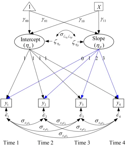
In this section, we briefly introduce the LGM with a variety of level-1 error covariance structures through a typical example depicted in Figure 1. In the figure, y1–y4 denote

repeated-measures on four occasions and X a level-2 predictor. i α

η is the random intercept representing the initial status for individual i, ηβ_i is the random slope showing the individual’s linear rate of change per unit increase in time. The first-level model can be written as * = _y + y Λ η ε, (1) where y=[ ]y y y y ′_{1 2 3 4} , * 1 2 3 4 1 2 3 4 1 1 1 1 1 1 1 1 T 1 T 1 T 1 T 1 λ λ λ λ ⎡ ⎤ ⎡ ⎤ ′ =_{⎢ ⎥ ⎢}= _{− − − − ⎥} ⎣ ⎦ ⎣ ⎦ y Λ , η=[ ]η ηα β ′, and 1 2 3 4 [ ]ε ε ε ε ′ =

ε . λ_t is the measurement time points (Tt = 1, 2, 3, 4), and ε denotes level-1

errors. The double-headed curved arrows presented in Figure 1 indicate that ε_t are correlated. The factor loading associated with initial status are all fixed at 1, whereas those associated with the slope are set at the valueλ_t to reflect the particular time point t for individual i . A common coding of λ_t for different time points is to set λ₁ = 0 for baseline

and 1λ_t = − for the follow-ups. For this model, subject i’s growth trajectory is a straight T_t

line, η_αi +λη_{t βi},λ_t= 0, 1, 2, 3.

--- Insert Figure 1 about here

---

The second-level model can be written as

0

=Γ +Γ x_x + _η

η ζ , (2)

where Γ₀ =[γ γ_{00 01}]′ , Γ_x =[γ γ_{10 11}]′ , x=

[ ]

10

γ denote, respectively, the intercept and slope of the regression of η_α on X, γ₀₁ and γ₁₁ are those of ηβ on X, and ζηα and ζηβ are level-2 errors. It is assumed that ζ and η ε are

uncorrelated. The models can be rewritten in combined form as

* * 0 ( ) y y η =Λ Γ +Γ x_x +Λ +ε y ζ , (3)

based on which the mean vector μ and the covariance matrix Σ of the manifest variables

y1–y4 and X can be expressed as functions of the model parameters as follows: (Bollen &

Curran, 2006, p.134-135): * 0 ( ) ⎡ + ⎤ ⎡ ⎤ =_{⎢ ⎥= ⎢ ⎥} ⎣ ⎦ ⎣ ⎦ y y x x x x Λ Γ Γ μ μ μ μ μ , (4) * * * * ( ) ⎡ _{′ +} ′₊ ⎤ ⎢ ⎥ = ⎢ _{′ ′} ⎥ ⎣ ⎦ y x xx x y y x xx xx x y xx Λ Γ Σ Γ Ψ Λ Θ Λ Γ Σ Σ Σ Γ Λ Σ η ζ ε , (5)

where Θε and Ψζηdenote the variance-covariance matrices of ε and ζη, respectively, and

x

μ and Σ denote, respectively the mean vector and the variance-covariance matrix of _xx predictors (μ_x =μ_X and 2

X

σ

= xx

The first-level errors,ε₁, ε₂, ε₃, and ε₄, are assumed to be normally distributed with zero means. The general form of the ECM is unstructured, and is given by

1 2 1 2 3 1 3 2 3 4 1 4 2 4 3 4 2 2 2 2 ε ε ε ε ε ε ε ε ε ε ε ε ε ε ε ε σ σ σ σ σ σ σ σ σ σ ⎡ ⎤ ⎢ ⎥ ⎢ ⎥ = ⎢ ⎥ ⎢ ⎥ ⎢ ⎥ ⎣ ⎦ Θε . (6)

The corresponding option given in SAS PROC MIXED is TYPE=UN. Other types of ECM, with less parameters (parsimonious) may be desirable. The chi-square test resulting from PROC CALIS (not available by PROC MIXED) can be used to help determine an appropriate type. The second-level errors ζ_ηα and ζ are assumed to be normally distributed with zero η_β

means. Their covariance matrix is usually specified as unstructured (Murphy & Pituch, 2009):

2 2 ηα ηα ηβ ηα ηβ ηβ ζ ζ ζ ζ ζ ζ σ σ σ σ ⎡ ⎤ ⎢ ⎥ = ⎢ ⎥ ⎣ ⎦ Ψ_ζη . (7)

Types of Level-1 Error Covariance Structures and SAS Statements

Any type of ECM, Θ or ε Ψζη, can be expressed as a set of linear and/or nonlinear constraints. The SAS statements by PROC CALIS for specifying six types of the first-level error covariance structure are summarized in Table 1. They include the first-order autoregressive (AR(1)), the first-order autoregressive moving-average (ARMA(1,1)), the second-order autoregressive (AR(2)), heterogeneous ARH(1), heterogeneous Toeplitz (TOEPH), and unstructured (UN), commonly considered in time series analysis and among which there exist nested relationships (Kwok, West, & Green, 2007). Stationarity is assumed for the first three processes, and should be examined to justify the use of the corresponding ECM.

--- Insert Table 1 about here

Statements by SAS PROC MIXED. PROC MIXED provides a REPEATED statement,

in which many types of the first-level error covariance structure can be specified through the TYPE= option (e.g., Singer, 1998).

Statements by SAS PROC CALIS. The STD, COV, and PARAMETERS statements in

PROC CALIS can be used together to specify any type of ECM (Θ or _ε

η

ζ

Ψ ). The PARAMETERS statement defines additional parameters that are not specified in the models, and uses both the original and additional parameters for modeling ECM. In other words, each specific type of ECM is composed of functions of the original and additional parameters.

Example 1: Θε Resulting from ARMA(1,1)

The ECM resulting from the stationary ARMA(1,1) process, defined as ε_t =φ ε_{1 t−1}+ −ν θν_{t 1 t−1}, where φ₁ denotes the autoregressive parameter, θ₁ the moving average parameter, and ν_t a white noise process (independent and identically distributed disturbances) (Box, Jenkins, & Reinsel, 1994, p.77), is given by 1 2 2 1 3 2 1 1 1 1 1 ε ρ σ ρ ρ ρ ρ ρ ⎡ ⎤ ⎢ ⎥ ⎢ ⎥ = ⎢ ⎥ ⎢ ⎥ ⎣ ⎦ Θε , (8) where 1 1 1 1 1 2 1 1 1 ( )(1 ) (1 2 ) φ θ φ θ ρ φ θ θ − − =

− + , ρk =φ ρ1 k−1, 2, k = 3, with the constraints of | | 1φ1 < and

1

|ρ | 1< . Program 1 in Appendix 1 illustrates how to use SAS PROC CALIS for modeling LGM with an ARMA(1,1) level-1 ECM and an unstructured level-2 ECM for four equally spaced time points. Under the assumption of stationarity for level-1 errors, their variances are equal, the autocovariances at lag 1 are equal, and the autocovariances at lag 2 are equal as well. Level-2 error variances/covariances are unstructured, as shown in Equation 7. Therefore, the STD and COV statements for specifying error variances and pairwise covariances are given as follows:

***************************************************************************; STD

E1=VARE, E2=VARE, E3=VARE, E4=VARE, D0=VARD0, D1=VARD1; COV

E1 E2=COV_lag1, E2 E3=COV_lag1, E3 E4=COV_lag1, E1 E3=COV_lag2, E2 E4=COV_lag2,

E1 E4=COV_lag3, D0 D1=COVD0D1;

***************************************************************************; In the STD statement, VARE represents the estimate of the common variance 2

ε

σ of the four level-1 errors ε₁–ε₄ (denoted by E1-E4), and VARD0 and VARD1 the estimates of the variances, 2 ηα ζ σ and 2 ηβ ζ

σ , of the two level-2 errors

α η ζ and β η ζ (denoted by D0 and D1).

In the COV statement, COV_lag1 and COV_lag2 represent, respectively, the common level-1 error autocovariance estimates at lag 1 and lag 2. COV_lag3 is the estimate of the error autocovariance at lag 3. CD0D1 is the estimate of

ηα ηβ

ζ ζ

σ . Parameters ρ₁ and φ₁ defined in

Equation 8 and their relationships with the autocovariances can be specified by using the following PARAMETERS statement. Starting values for estimating ρ₁ and φ₁ are needed and should appear in the parenthesis. Population parameters are used as starting values to achieve convergence more efficiently for simulation studies (Paxton, Curran, Bollen, Kirby, & Chen, 2001).

***************************************************************************; PARAMETERS

PHI1 RHO1 (0.6 0.7); COV_lag1=RHO1*VARE;

COV_lag2=PHI1* COV_lag1; /* i.e., COV_lag2=PHI1*RHO1* VARE; */ COV_lag3=PHI1* COV_lag2; /* i.e., COV_lag3=(PHI1**2)*RHO1*VARE; */

***************************************************************************; ‘COV_lag1=RHO*VARE’ corresponds to the requirement that the common autocovariance at lag 1 be equal to 2

1 ε

σ ρ . The syntax corresponding to the requirements for the common autocovariances at lag 2 (= 2 1 1 ε σ φ ρ ) and lag 3 (= 2 2 2 1 2 1 1 ε ε

The constraints of | | 1φ₁ < and |ρ₁| 1< are specified by the following BOUNDS statement: ***************************************************************************; BOUNDS

–1. < PHI1 < 1., –1. < RHO1 < 1.;

***************************************************************************;

Example 2: Θε Resulting from TOEPH

The ECM resulting from heterogeneous Toeplitz is given by

1 2 1 2 3 1 3 2 3 4 1 4 2 4 3 4 2 2 1 2 2 1 2 3 2 1 ε ε ε ε ε ε ε ε ε ε ε ε ε ε ε ε

σ

σ σ ρ

σ

σ σ ρ σ σ ρ

σ

σ σ ρ σ σ ρ σ σ ρ σ

σ denotes the standard deviation forε_t, t = 1, 2, 3, 4, and ρ_j the autocorrelation at lag j, j = 1, 2, 3, with the constraints of |ρ_j | 1< , j = 1, 2, 3. The level-1 error variances are allowed to be unequal but the autocorrelations at the same lag are equal. The STD and COV statements used for specifying estimates of error variances and pairwise covariances are given as follows:

***************************************************************************; STD

E1=VARE1, E2=VARE2, E3=VARE3, E4=VARE4, D0=VARD0, D1=VARD1;

COV

E1 E2=COVE1E2, E1 E3=COVE1E3, E1 E4=COVE1E4, E2 E3=COVE2E3, E2 E4=COVE2E4, E3 E4=COVE3E4,

D0 D1=COVD0D1;

***************************************************************************; VARE1–VARE4 represent the estimates of the four level-1 error variances, and VARD0 and VARD1 those of the two level-2 error variances. COVE1E2–COVE3E4 represent the corresponding level-1 error autocovariance estimates, and COVD0D1 the level-2 error autocovariance estimate. Since σε ε_{t t}′ =σ σ ρε_t ε_t′ ε ε_{t t}′and the autocorrelations at the same lag are

constrained to be equal, the following PARAMETERS statement needs to be added:

***************************************************************************; PARAMETERS

RHO1 RHO2 RHO3 (0.7 0.6 0.7);

COVE1E2=SQRT(VARE1)*SQRT(VARE2)*RHO1; COVE1E3=SQRT(VARE1)*SQRT(VARE3)*RHO2; COVE1E4=SQRT(VARE1)*SQRT(VARE4)*RHO3; COVE2E3=SQRT(VARE2)*SQRT(VARE3)*RHO1; COVE2E4=SQRT(VARE2)*SQRT(VARE4)*RHO2; COVE3E4=SQRT(VARE3)*SQRT(VARE4)*RHO1; ***************************************************************************; The constraints of |ρ_j| 1< ( j = 1, 2, 3) can be handled by using the BOUNDS statement given below.

***************************************************************************; BOUNDS

–1. < RHO1 < 1. , –1.< RHO2 <1., –1.< RHO3 < 1.;

***************************************************************************; The LINEQS statement used for this example is the same as that given in Example 1.

Although there are many defaulted error covariance structures in PROC MIXED, modification is not allowed for any of them. In contrast, PROC CALIS can be used to specify any error covariance structure to meet researchers’ need. For example, the AR(2) process, given by ε_t =φ ε_{1 t−1}+φ ε_{2 t−2}+ , where ν_t φ₁ and φ₂ are autoregressive parameters and ν_t a white noise process (Box, Jenkins, & Reinsel, 1994, p.54), leads to the following level-1 ECM: 1 2 2 1 3 2 1 1 1 1 1 ε ρ σ ρ ρ ρ ρ ρ ⎡ ⎤ ⎢ ⎥ ⎢ ⎥ ⎢ ⎥ ⎢ ⎥ ⎣ ⎦ , (10)

where ρ₀ = 1, ρ φ₁= ₁/ (1−φ₂), and ρ_k =φ ρ_{1 k−1}+φ ρ_{2 k−2}, 2, k= 3, with the constraints of

2

|φ | 1< , φ φ₂+ < , and ₁ 1 φ φ₂− < . It is not possible to model AR(2) for level-1 errors by ₁ 1 using PROC MIXED, but the task can be done by using PROC CALIS, with the statements shown in Table 1. Note that the last two constraints are specified by using the LINCON

statement. PROC CALIS is certainly more flexible than PROC MIXED.

SAS statements by PROC CALIS for modeling other types of stationary and nonstationary level-1 error processes such as those presented in Appendix 3 can be obtained in a similar way.

AN EFFECTIVE APPROACH FOR IDENTIFYING THE FIRST-LEVEL ERROR COVARIANCE STRUCTURE

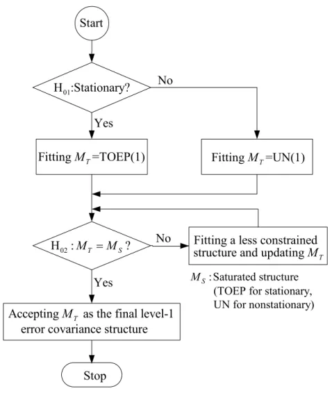
By following the sequential chi-square difference test (SCDT) given by Anderson and Gerbing (1988), an effective approach is proposed to identify the first-level error covariance structure as follows:

Stage 1: Testing for stationarity of the first-level error process.

The conditions of stationarity include the equality of error variances and the equality of error autocovariances at any lag (Box, Jenkins, & Reinsel, 1994, p. 24-26). For example, for the model shown in Figure 1, the null hypothesis of stationarity is given by H01:

1 2 3 4 2 1 3 2 4 3 3 1 4 2

2 2 2 2_{, , .}

ε ε ε ε ε ε ε ε ε ε ε ε ε ε

σ

σ

σ

σ

σ

σ

σ

σ

σ

SIMTEST statement in PROC TCALIS, in addition to the STD and COV statements given in Example 2, as follows:

***************************************************************************; SIMTEST ERR_STATIONARY_TEST = [VAREQ_1 VAREQ_2 VAREQ_3

COVLag1EQ_1 COVLag1EQ_2 COVLag2EQ]; VAREQ_1=VARE1–VARE2; VAREQ_2=VARE1–VARE3; VAREQ_3=VARE1–VARE4; COVLag1EQ_1=COVE1E2–COVE2E3; COVLag1EQ_2=COVE1E2–COVE3E4; COVLag2EQ=COVE1E3–COVE2E4; ***************************************************************************; The null hypothesis given above can be reexpressed as H01:σ_ε2₁−σ_ε2₂ =0, σ_ε2₁−σ_ε2₃ =0,

1 4 2 2 _0, ε ε σ −σ = 2 1 3 2 0, ε ε ε ε σ −σ = 2 1 4 3 0, ε ε ε ε σ −σ = 3 1 4 2 0, ε ε ε ε

σ −σ = in which six functions of the model parameters, named VAREQ_1, VAREQ_2, VAREQ_3, COVLag1EQ_1, COVLag1EQ_2, and COVLag2EQ, respectively, are all equal to zero. To conduct a simultaneous test for the six functions by using the SIMTEST statement, we first assign a

name, ERR_STATIONARY_TEST, for the test, and then put the function names inside a pair of brackets ‘[’ and ‘]’. The six functions are defined in the SAS programming statements, and follow after the SIMTEST statement. VAREQ_1, VAREQ_2, and VAREQ_3 represent the differences between

1

2

ε

σ and each of the other error variances. COVLag1EQ_1 and COVLag1EQ_2 represent, respectively, σ_{ε ε2 1} −σ_{ε ε3 2} and σ_{ε ε2 1} −σ_{ε ε4 3} , the two pairwise comparisons among the three error covariances at lag 1. COVLag2EQ is the contrast between the two error covariances at lag 2. The SIMTEST statement would lead to a chi-square test (with 6 degrees of freedom) for examining stationarity.

If stationarity is supported, then go to Stage 2A; otherwise go to Stage 2B. Stage 2A: Identifying the type of stationary process using SCDT.

We fit the model with stationary level-1 error processes sequentially, starting from TOEP(1), the most constrained one (the most parsimonious stationary one as well), followed by the order of AR(1), (ARMA(1,1) or AR(2)), and TOEP, according to the degree of constraint. TOEP, the least constrained (the least parsimonious) structure, is actually the saturated stationary one. At each step, we first test if the model fit using the current structure, denoted by MT, is significantly different from the model fit using TOEP, denoted by MS, with

the chi-square difference test. The difference of the chi-square statistic for MT and that for MS

is distributed as a chi-square distribution with degrees of freedom equaling the difference of the number of parameters within the two ECM. The significant result indicates that the current MT possesses significantly worse model fit, and we enter the next step by updating MT

with a less constrained structure. The test is continued until the fit does not show significant difference (denoted as MT − MS = 0), and MT is the error covariance structure we need.

Stage 2B: Identifying the type of nonstationary process using SCDT.

The SCDT is conducted for nonstationary processes in a similar way as Stage 2A, following the order of UN(1), ARH(1), TOEPH, and UN. UN(1) is the most parsimonious of all. UN is the saturated structure.

The reasons to recommend TOEP(1), AR(1), (ARMA(1,1) or AR(2)), and TOEP in Stage 2A, and UN(1), ARH(1), TOEPH, and UN in Stage 2B are simply because they are nested and easy to interpret. More detailed structures may also be used if they can meet the same conditions. A flow chart for identifying the first-level error covariance structure is given in Figure 3.

Illustrations

Two illustrations are given. The first one is based on the data generated from the linear growth model shown in Figure 1 with the TOEPH level-1 error structure and the UN level-2 error structure. Population parameters and the sample covariance matrix of y1–y4 and X are

given in Table 2. The sample size of 300 was used (Muthén & Muthén, 2002).

--- Insert Table 2 about here

---

Following the approach for identifying the first-level error covariance structure, we first test for stationarity. Since stationarity was rejected ( 2

6

df

χ ₌ =123.93, p <.0001), we proceeded with a specification search for a nonstationary process. Error covariance structures were fit sequentially. We started by fitting UN(1). Since the model fit between UN(1) and UN was significant (chi-square difference = 15.903 with df = 6, p = .014), UN(1) should not be adopted. Then we fit ARH(1), a less constrained one. Since the model fit between ARH(1) and UN became insignificant (chi-square difference = .441 with df = 5, p = .994), the sequential search was terminated by choosing ARH(1) as the first-level error covariance structure. The improvement of ARH(1) over UN(1) can be verified by the significant results between UN(1) and ARH(1) (chi-square difference = 15.462 with df = 1, p <.0001). Although the final structure identified, ARH(1), is not the one specified in the population model (TOEPH), their performance in model fit was insignificant (chi-square difference = .441 with df = 2, p = .802). ARH(1) is preferred since it is more parsimonious (with two less parameters). The results of SCDT are summarized in Table 3. The parameter estimates of the final model (with ARH(1)) are also reported in the same table by using both PROC CALIS (the SEM approach) and PROC MIXED (the HLM approach) for the purpose of verification. It appears that parameter estimates resulting from the two approaches are pretty close. The model fit was satisfactory ( 2

6

df

χ ₌ = 1.483, p = .961, AGFI = .996, RMSEA = .000). However, the test for stationarity and the sequential chi-square difference tests that can be implemented by PROC CALIS cannot work under PROC MIXED. Moreover, while the estimates of Θ_ε and Ψ_ζηcould be obtained by both PROC MIXED and PROC CALIS, the significance test for error covariances can be achieved by PROC CALIS only. Two approaches yield about the

same results when PROC MIXED works. PROC CALIS supplies richer information in model fit and parameter inference.

--- Insert Table 3 about here

---

The second illustration is based on the data given in Singer and Willett (2003, Chap. 7). 35 people completed an inventory measuring their performance on a timed task called “opposite’s naming” on each of four days, spaced exactly one week apart. At wave 1, they also completed a standardized instrument assessing general cognitive skill, used as a subject-level predictor. The growth model used is exactly the one shown in Figure 1. Since stationarity was not rejected ( 2

6

df

χ ₌ =3.302, p = .77), the covariance structure to be identified should come from the pool of stationary processes. Error covariance structures were fit sequentially, by using TOEP(1) in the first step. The results are summarized in Table 4. Since the model fit between TOEP(1) and TOEP was insignificant (chi-square difference = 2.801 with df = 4, p = .592), no further examination was needed, and we selected TOEP(1) to be the first-level error covariance structure. The level-1 errors were uncorrelated and identically distributed in this case. The model fit was good ( 2

10

df

χ ₌ = 6.68, p = .755, AGFI = .987, RMSEA = .000). The parameter estimates by fitting TOEP(1) are also given in the same table by using both PROC CALIS and PROC MIXED. Again, the results are close to each other.

--- Insert Table 4 about here

---

SECOND-ORDER LATENT GROWTH MODELS

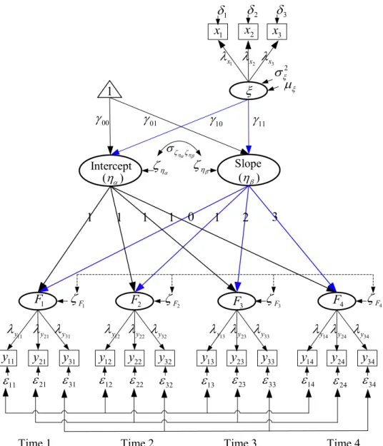
When the growth trajectory is to be analyzed for a latent construct, measured with multiple indicators, only the SEM approach can work, based on the second-order LGM (e.g. Bollen & Curran, 2006, Chap. 8; Hancock, Kuo, & Lawrence, 2001; Preacher et al., 2008, Chap. 3; Sayer & Cumsille, 2001). In Figure 2, latent construct F is measured with three indicators,

y1–y3, which are observed at four occasions. The constructs at the four occasions, denoted by

1

denoted by η_α and η_β , are termed the second-order factors. There exist a predictor construct, ξ, for the growth factors, and it is measured with three indicators, x1–x3. The errors

associated with the indicators y1–y3, εjt, j = 1, 2, 3; t = 1, 2, 3, 4, and those associated with

the first-order factors,

1 4

F F

ζ −ζ , are level-1 errors. The errors associated with the second-order factors, ζη_α and ζηβ , and those associated with the indicators x1–x3 , δ1–δ3, are

level-2 errors. The level-1 errors associated with the same indicator at different points in time (ε_j1−ε_j4, j = 1, 2, 3) are serially correlated. They are linked in the figure by three solid lines with four arrowheads, one line for each indicator.

1 4

F F

ζ −ζ are serially correlated as well (Sivo, 2001). They are linked by a dash line with four arrowheads. Their covariance structures need to be well identified, and can be done by using the approach proposed in the previous section. Other errors are assumed to be uncorrelated.

--- Insert Figure 2 about here

---

The second-order LGM pictorially presented in Figure 2 can be represented in matrix form as follows: * 0 , , , , ξ ξ ξ = + = + = + = + + y x y y Λ x Λ Λ ζ Γ Γ ζ F η F δ F η η ε (11) where y=[y y y y y y y y y y y y11 ] ,21 31 12 22 32 13 23 33 14 24 34 ′x=[ ] , [ ] , [ ] ,x x x1 2 3 ′ F = F F F F1 2 3 4 ′ η = η ηα β ′ 11 21 31 12 22 32 13 23 33 14 24 34 [ε ε ε ε ε ε ε ε ε ε ε ε ]′ = ε , δ =[ ]δ δ δ_{1 2 3} ′, 1 2 3 4 [ζ ζ ζ ζ_{F F F F} ]′ = ζ_F , and [ζ ζ ]η_α η_β ′ =

ζη . Λ and y Λx denote the loading matrices in the measurement model,Λ*y denotes the loading matrix in the growth model, and Γ₀ and Γ_ξ denote, respectively, the vector of intercepts and slopes of the regressions of the growth factors η on the predictor construct ξ . They are specifically shown in Table 5. It is assumed that ( )E ε =E( )δ =

( ) ( )

E ζ_F =E ζ_η =0 , Cov ξ( , )δ =Cov ξ( , )ζ_η =Cov ξ( ,ζ_F)=Cov ξ( , )ε =0 , and Cov( , )ε δ =

( , ) ( , ) ( , ) ( , ) ( , )

0, j ≠ j’. Let Θ_ε, Ψ η

ζ , ΨζF , and Φξ denote, respectively, the variance-covariance matrices of ε , ζη, ζF, and ξ . The implied mean vector and the variance-covariance matrix of y and x are given in Appendix 2. Because Θ_ε and Ψ

F

ζ involve time occasions, their covariance

structures need to be identified. Since the four level-1 error processes, ε₁ =[ε ε ε ε_{11 12} ]_{13 14} ′,

2 =[ε ε ε ε21 22 23 24]′

ε , ε₃ =[ε ε ε ε_{31 32 33 34}]′, and ζ_F =[ζ ζ ζ ζ ]_{F1 F2 F3 F4} ′, associated with the

indicators y1–y3 and the construct F, respectively, are assumed to be uncorrelated, the

approach proposed previously for identifying the first-level error covariance structure can be used individually for each of them. However, the assumption of the uncorrelatedness of ε₁,

2

ε , and ε₃ may be violated due to systematic effects. The chi-square difference test can be used to test for the assumption.

--- Insert Table 5 about here

--- Statements by SAS PROC CALIS/TCALIS

SAS Program 2 in Appendix 2 are used for fitting AR(1) for ε j (j = 1, 2, 3) (the first-level

errors associated with the same indicator across four time points) and ζF (the first-level errors associated with the construct across four time points), and fitting UN for ζ_η(the second-level errors) by using SAS PROC CALIS. There are two parameters in AR(1) for each error process. The parameters to be estimated simultaneously include 2

j ε σ , ₁ j ε φ , j = 1, 2, 3, and 2 F ς σ , ₁ F ζ

φ . The assumption of stationarity requires that | ₁ | 1

j ε φ < and | ₁ | 1 F ζ φ < .

In the STD statement, the first-level error variance estimates associated with the same indicator/the construct are set equal across time by using the same names. In the COV statement, we specify the same name for the lag-1 autocovariances to each indicator and the construct, and similarly for the lag-2 autocovariances. In the PARAMETERS statement, the additional covariance structure parameters for AR(1) need to be defined first, one for each indicator and the construct (i.e., ₁

j

ε

φ and φ_1ζF), with initial values given in the parentheses, and then SAS programming statements are used to specify the relationships among the parameters delineating the particular error covariance structure for all indicators and the

construct. The principles are exactly the same as before. The requirements of ‘| ₁ | 1

j

ε

φ < and

1

|φ_ζF | 1< ’ are specified by the BOUNDS statement.

The approach proposed for identifying the error covariance structure is also applicable for the second-order LGM. The first stage is to test, for stationarity,

11 12 13 14 12 11 13 12 14 13 13 11 14 12 21 22 23 24 22 21 23 22 24 23 23 21 24 22 31 32 33 34 32 31 33 32 34 33 2 2 2 2 01_1 2 2 2 2 01_ 2 2 2 2 2 01_ 3 H : , , , H : , , , H : , , ε ε ε ε ε ε ε ε ε ε ε ε ε ε ε ε ε ε ε ε ε ε ε ε ε ε ε ε ε ε ε ε ε ε ε ε ε ε σ σ σ σ σ σ σ σ σ σ σ σ σ σ σ σ σ σ σ σ σ σ σ σ σ = = = = = = = = = = = = = = = = = 33 31 34 32, ε ε ε ε σ =σ and 1 2 3 4 2 1 3 2 4 3 3 1 4 2 2 2 2 2 01_ 4 H : , , , F F F F F F F F F F F F F F ς ς ς ς ς ς ς ς ς ς ς ς ς ς σ =σ =σ =σ σ =σ =σ σ =σ

individually for each of the first-level error processes, ε ε ε₁, , ,_{2 3} and ζ_F,by using the SIMTEST statement in PROC TCALIS mentioned in the previous section, followed by the steps in stage 2A for identifying the specific stationary error process or in stage 2B for identifying the specific nonstationary error process using SCDT.

Illustration

We demonstrate identifying the covariance structures of Θ_ε and Ψ_ζ

F with another dataset of size 300 generated from the second-order LGM in Figure 2. The population parameters with the AR(1) covariance structure for level-1 error processes ε₁, ε₂, ε₃, and ζF and the sample covariance matrix of y and x resulting from the simulated dataset are presented in Table 5. The RANDNORMAL function in PROC IML (SAS 9.2) was used to generate multivariate

normal data. Since the uncorrelatedness of ε₁, ε₂, and ε₃ was supported (chi-square difference = 30.866 with df = 48, p = .97408), stationarity could be assessed and specification

search could be conducted individually. Since stationarity was further supported for all ε₁,

2

ε , ε₃, and ζF (

χ

=

we proceeded to search for stationary structures. When identifying the first-level ECM for a specific error process, TOEP was specified for the other three processes. The results of SCDT are reported in Table 6. AR(1) was identified for ε₁, ε₂, ε₃, and TOEP(1) for ζF. The parameter estimates by fitting AR(1) for ε₁, ε₂, ε₃ and TOEP(1) for ζF were close to the

population parameters specified in Table 5. The model fit was satisfactory ( 2 112 df χ ₌ = 107.53, p = .602, AGFI = .996, RMSEA = .000). --- Insert Table 6 about here

---CONCLUSION

This article illustrates the use of the SAS PROC CALIS/TCALIS to fit error covariance structure of latent growth models. A tutorial on the syntax has been provided for both manifest variables and latent constructs. An effective approach for identifying the first-level error covariance structure based on the sequential chi-square difference test has been proposed and demonstrated. In particular, how to test for stationarity of an error process, not discussed in the SEM or HLM literature, was specifically addressed. The illustrations based on simulated data have well reflected the effectiveness of the approach for identifying the error covariance structures. It is our hope that the approach proposed will help applied researchers obtain a better understanding about the specification of error covariance structure in latent growth models.

The joint use of the STD, COV, PARAMETERS, LINCON, and BOUNDS statements in PROC CALIS can be extended for other types of ECM in a similar way to meet analysts’ need. However, there exist some limitations. First, the design underlying LGM should be balanced. Second, time points should be equally spaced when testing for stationarity. Third, large samples are required to justify the use of SEM. In addition, if the errors associated with different indicators at the same occasion in the second-order LGM are correlated, a joint test for stationarity should be conducted, and the SCDT for identifying error covariance structures should also be carried out simultaneously. How to deal with these situations needs to be further studied.

REFERENCES

Anderson, J. C., & Gerbing, D. W. (1988). Structural equation modeling in practice: A review and recommended two-step approach. Psychological Bulletin, 103, 411–423.

Bauer, D. J. (2003). Estimating multilevel linear models as structural models. Journal of Educational and Behavioral Statistics, 28, 135–167.

Bentler, P. M., & Wu, E. J. C. (2005). EQS 6.1 - Structural equation modeling software for windows. Encino, CA: Multivariate Software, Inc.

Bollen, K. A., & Curran, P. J. (2006). Latent curve models: A structural equation perspective.

Hoboken, NJ: Wiley & Sons.

Box, G. E. P., Jenkins, G. M., & Reinsel, G. C. (1994). Time series analysis: Forecasting and control (3rd ed.). Englewood Cliffs, NJ: Prentice-Hall.

Chan, D. (1998). The conceptualization and analysis of change over time: An integrative approach incorporating longitudinal mean and covariance structures analysis (LMACS) and multiple indicator latent growth modeling (MLGM). Organizational Research Methods, 1, 421–483

Curran, P. J. (2003). Have multilevel models been structural equation models all along?

Multivariate Behavioral Research, 38, 529–569.

Duncan, S. C., Duncan, T. E., & Hops, H. (1996). Analysis of longitudinal data within accelerated longitudinal design. Psychological Methods, 1, 236–248.

Duncan, T. E., Duncan, S. C. & Strycker, L. A. (2006). An introduction to latent variable growth curve modeling: Concepts, issues, and applications (2nd ed.). Mahwah, NJ:

Lawrence Erlbaum Associates, Inc.

Ferron, J., Dailey, R. F., & Yi, Q. (2002). Effects of misspecifying the first-level error structure in two-level models of change. Multivariate Behavioral Research, 37, 379-403.

Hancock, G. R., Kuo, W. L., & Lawrence, F. R. (2001). An illustration of second-order latent growth models. Structural Equation Modeling, 8, 470–489.

Joreskog, K., & Sorbom, D. (2004). LISREL 8: User’s reference guide, Chicago: Scientific

Software International.

Kwok, O. M., West, S. G., & Green, S. B. (2007). The impact of misspecifying the within-subject covariance structure in multiwave longitudinal multilevel models: A Monte Carlo study. Multivaraite Behavioral Research, 42, 557–592.

MacCallum, R. C., Kim, C, Malarkey, W. B., and Kiecolt-Glaser, J. K. (1997). Studying multivariate change using multilevel models and latent curve models. Multivariate Behavioral Research, 32, 215–253.

Mehta, P. D., & Neale, M. C. (2005). People are variables too: Multilevel structural equations modeling, Psychological Methods, 10, 259–284.

Murphy, D. L., & Pituch, K. A. (2009). The Performance of multilevel growth curve models under an autoregressive moving average process. Journal of Experimental Education, 77,

255–282.

Muthén, B. O., & Khoo, S. T. (1998). Longitudinal studies of achievement growth using latent variable modeling. Learning and Individual Differences, 10, 73–101.

Muthén, L. K., & Muthén, B. O. (2002). How to use a Monte Carlo study to decide on sample size and determine power. Structural Equation Modeling, 9, 599–620.

Muthén, L. K., & Muthén, B. O. (2007). Mplus user’s guide (5th ed.). Los Angeles, CA:

Author.

Neale, M. C., Boker, S. M., Xie, G., & Maes, H. H. (2003). Mx: Statistical modeling (6th ed.).

Richmond: Virginia Commonwealth University.

Newsom, J. T. (2002). A multilevel structural equation model for dyadic data. Structural Equation Modeling, 9, 431–447.

Paxton, P., Curran, P. J., Bollen, K. A., Kirby, J., & Chen, F. (2001). Monte Carlo experiments: Design and implementation. Structural Equation Modeling, 8, 287–312.

Preacher, K. J., Wichman, A. L., MacCallum, R. C., & Briggs, N. E. (2008). Latent growth curve modeling. Thousand Oaks, CA: Sage.

Raudenbush, S. W. (2001). Comparing personal trajectories and drawing causal inferences from longitudinal data. Annual Review of Psychology, 52, 501–525.

Raudenbush, S., Bryk, A., & Congdon, R. (2005). HLM for Windows (version 6.03).

Lincolnwood, IL: Scientific Software International.

Rovine, M. J., & Molenaar, P. C. M. (2000). A structural modeling approach to a multilevel random coefficients model. Multivariate Behavioral Research, 35, 51–88.

Sayer, A. G., & Cumsille, P. E. (2001). Second-order latent growth models. In L. Collins & AG Sayer (Eds.), New methods for the analysis of change (pp. 179-200). Washington DC:

American Psychological Association.

SAS Institute Inc. (2007). SAS/STAT user’s guide (SAS 9.2). Cary, NC: Author.

Singer, J. D. (1998). Using SAS PROC MIXED to fit multilevel models, hierarchical models, and individual growth models. Journal of Educational and Behavioral Statistics, 24,

323–355.

Singer, J. D., & Willett, J. B. (2003). Applied longitudinal data analysis: Modeling change and event occurrence. New York: Oxford University Press.

Sivo, S. (2001). Multiple Indicator Stationary Time Series Models. Structural Equation Modeling, 8, 599–612.

Sivo, S., Fan, X., & Witta, L. (2005). The biasing effects of unmodeled ARMA time series processes on latent growth curve model estimates. Structural Equation Modeling, 12,

215–231.

Sivo, S., & Fan, X. (2008). The latent curve ARMA (p, q) panel model: Longitudinal data

analysis in educational research and evaluation. Educational Research and Evaluation, 14,

363–376.

Willett, J. B., & Sayer, A. G. (1994). Using covariance structure analysis to detect correlates

and predictors of individual change over time. Psychological Bulletin, 116, 363–381.

Wolfinger, R. (1996). Covariance structures for repeated measures. Journal of Agricultural, Biological, and Environmental Statistics, 1, 205–230.

TABLE 1

SAS Statements in PROC CALIS for Specifying Different Types of the First-Level Error Covariance Structure with Four Occasions

Structure ( Θ_ε) Statements in PROC CALIS

AR(1) (first-order autoregressive): 1 1 t t t ε =φ ε₋ + , ν 1 2 2 1 1 3 2 1 1 1 1 1 1 1 ε φ σ φ φ φ φ φ ⎡ ⎤ ⎢ ⎥ ⎢ ⎥ ⎢ ⎥ ⎢ ⎥ ⎣ ⎦ , 1 | | 1φ < . STD

E1=VARE, E2=VARE, E3=VARE, E4=VARE, D0 =VARD0, D1 =VARD1;

COV

E1 E2=COV_lag1, E2 E3=COV_lag1, E3 E4=COV_lag1, E1 E3=COV_lag2, E2 E4=COV_lag2, E1 E4=COV_lag3, D0 D1=CD0D1;

PARAMETERS PHI1 (0.6);

COV_lag1= PHI1*VARE; COV_lag2=(PHI1**2)*VARE; COV_lag3= (PHI1**3) *VARE;

BOUNDS

–1. < PHI1 < 1. ;

ARMA(1,1) (first-order

autoregressive moving average): 1 1 1 1 t t t t ε =φ ε₋ + −ν θν ₋ , 1 2 2 1 3 2 1 1 1 1 1 ε ρ σ ρ ρ ρ ρ ρ ⎡ ⎤ ⎢ ⎥ ⎢ ⎥ ⎢ ⎥ ⎢ ⎥ ⎣ ⎦ , 1 1 1 1 1 2 1 1 1 1 1 1 1 ( )(1 ) , (1 2 ) , 2, 3, | | 1, | | 1. k k k φ θ φ θ ρ φ θ θ ρ φ ρ ₋ φ ρ − − = − + = = < < STD

E1=VARE, E2=VARE, E3=VARE, E4=VARE, D0=VARD0, D1=VARD1;

COV

E1 E2=COV_lag1, E2 E3=COV_lag1, E3 E4=COV_lag1, E1 E3=COV_lag2, E2 E4=COV_lag2, E1 E4=COV_lag3, D0 D1=CD0D1;

PARAMETERS PHI1 RHO1 (0.6 0.7) ;

COV_lag1=RHO1*VARE; COV_lag2=PHI1* COV_lag1; COV_lag3=PHI1* COV_lag2;

BOUNDS

–1. < PHI1 < 1., –1. < RHO1 < 1. ;

AR(2) (second-order AR): 1 1 2 2 t t t t ε =φ ε ₋ +φ ε ₋ + , ν 1 2 2 1 3 2 1 1 1 1 1 ε ρ σ ρ ρ ρ ρ ρ ⎡ ⎤ ⎢ ⎥ ⎢ ⎥ ⎢ ⎥ ⎢ ⎥ ⎣ ⎦ , 0 1, 1 1/ (1 2) ρ = ρ φ= −φ , 1 1 2 2, 2, 3, k k k k ρ =φ ρ ₋ +φ ρ ₋ = 2 |φ | 1< , φ φ₂+ < , ₁ 1 φ φ₂− < . ₁ 1 STD

E1=VARE, E2=VARE, E3=VARE, E4=VARE, D0=VARD0, D1=VARD1;

COV

E1 E2=COV_lag1, E2 E3=COV_lag1, E3 E4=COV_lag1, E1 E3=COV_lag2, E2 E4=COV_lag2, E1 E4=COV_lag3, D0 D1=CD0D1;

PARAMETERS PHI1 PHI2 (0.5 0.4);

RHO1= PHI1/(1–PHI2); COV_lag1=RHO1*VARE;

COV_lag2=PHI1*COV_lag1+ PHI2 *VARE; COV_lag3=PHI1*COV_lag2+PHI2*COV_lag1;

LINCON

PHI2 + PHI1 < 1., PHI2 –PHI1 < 1.;

BOUNDS

TABLE 1 (Continued)

Structure Statements in PROC CALIS

UN (unstructured): 1 2 1 2 3 1 3 2 3 4 1 4 2 4 3 4 2 2 2 2 ε ε ε ε ε ε ε ε ε ε ε ε ε ε ε ε σ σ σ σ σ σ σ σ σ σ ⎡ ⎤ ⎢ ⎥ ⎢ ⎥ ⎢ ⎥ ⎢ ⎥ ⎢ ⎥ ⎢ ⎥ ⎣ ⎦ STD

E1=VARE1, E2=VARE2, E3=VARE3, E4=VARE4, D0=VARD0, D1=VARD1;

COV

E1 E2=COVE1E2, E1 E3=COVE1E3, E1 E4=COVE1E4, E2 E3=COVE2E3, E2 E4=COVE2E4, E3 E4=COVE3E4,

D0 D1=CD0D1;

TOEPH (heterogeneous Toeplitz):

1 2 1 2 3 1 3 2 3 4 1 4 2 4 3 4 2 2 1 2 2 1 2 3 2 1 ε ε ε ε ε ε ε ε ε ε ε ε ε ε ε ε σ σ σ ρ σ σ σ ρ σ σ ρ σ σ σ ρ σ σ ρ σ σ ρ σ ⎡ ⎤ ⎢ ⎥ ⎢ ⎥ ⎢ ⎥ ⎢ ⎥ ⎢ ⎥ ⎣ ⎦ , 1 2 3 |ρ | 1, |< ρ | 1, |< ρ | 1< STD

E1=VARE1, E2=VARE2, E3=VARE3, E4=VARE4, D0=VARD0, D1=VARD1;

COV

E1 E2=COVE1E2, E1 E3=COVE1E3, E1 E4=COVE1E4, E2 E3=COVE2E3, E2 E4=COVE2E4, E3 E4=COVE3E4,

D0 D1=CD0D1;

PARAMETERS RHO1 RHO2 RHO3 (0.7 0.6 0.7);

COVE1E2=SQRT(VARE1)*SQRT(VARE2)*RHO1; COVE1E3=SQRT(VARE1)*SQRT(VARE3)*RHO2; COVE1E4=SQRT(VARE1)*SQRT(VARE4)*RHO3; COVE2E3=SQRT(VARE2)*SQRT(VARE3)*RHO1; COVE2E4=SQRT(VARE2)*SQRT(VARE4)*RHO2; COVE3E4=SQRT(VARE3)*SQRT(VARE4)*RHO1; BOUNDS

–1. < RHO1 < 1. , –1.< RHO2 <1., –1.< RHO3 < 1.;

ARH(1) (heterogeneous AR(1)):

1 2 1 2 3 1 3 2 3 4 1 4 2 4 3 4 2 2 2 2 3 2 2 ε ε ε ε ε ε ε ε ε ε ε ε ε ε ε ε σ σ σ ρ σ σ σ ρ σ σ ρ σ σ σ ρ σ σ ρ σ σ ρ σ ⎡ ⎤ ⎢ ⎥ ⎢ ⎥ ⎢ ⎥ ⎢ ⎥ ⎢ ⎥ ⎣ ⎦ , | | 1ρ < STD

E1=VARE1, E2=VARE2, E3=VARE3, E4=VARE4, D0=VARD0, D1=VARD1;

COV

E1 E2=COVE1E2, E1 E3=COVE1E3, E1 E4=COVE1E4, E2 E3=COVE2E3, E2 E4=COVE2E4, E3 E4=COVE3E4,

D0 D1=CD0D1; PARAMETERS RHO (0.7); COVE1E2=SQRT(VARE1)*SQRT(VARE2)*RHO; COVE1E3=SQRT(VARE1)*SQRT(VARE3)*RHO**2; COVE1E4=SQRT(VARE1)*SQRT(VARE4)*RHO**3; COVE2E3=SQRT(VARE2)*SQRT(VARE3)*RHO; COVE2E4=SQRT(VARE2)*SQRT(VARE4)*RHO**2; COVE3E4=SQRT(VARE3)*SQRT(VARE4)*RHO; BOUNDS –1. < RHO < 1.;

Note. The second-level ECM,

2 2 ηα η ηα ηβ ηβ ζ ζ ζ ζ σ σ σ ⎡ ⎤ ⎢ ⎥ = ⎢ ⎥ ⎣ ⎦ ζ

TABLE 2

Population Parameters of the Model in Figure 1 Based on the First-Level Error Covariance Structure of TOEPH and the Sample Covariance Matrix of y1–y4 and X Resulting from a

Dataset of Size 300 Generated from the Model

* 1 0 1 1 1 2 1 3 ⎡ ⎤ ⎢ ⎥ = ⎢ ⎥ ⎢ ⎥ ⎣ ⎦ y Λ , 01 11 4 6 γ γ ⎡ ⎤ ⎡ ⎤ =_{⎢ ⎥ ⎢ ⎥}= ⎣ ⎦ ⎣ ⎦ x Γ , 2 ₁ X σ = = xx Σ , 0μ_x =μ_X = , 00 0 10 10 4 γ γ ⎡ ⎤ ⎡ ⎤ =_{⎢ ⎥ ⎢ ⎥}= ⎣ ⎦ ⎣ ⎦ Γ , 2 2 15 7 10 ηα ηα ηβ ηβ ζ ζ ζ ζ σ σ σ ⎡ _{⎤ ⎡ ⎤} ⎢ ⎥ = _{= ⎢ ⎥} ⎢ _{⎥ ⎣ ⎦} ⎣ ⎦ Ψ η ζ , 1 2 1 2 3 1 3 2 3 4 1 4 2 4 3 4 2 2 1 2 2 1 2 3 2 1 ε ε ε ε ε ε ε ε ε ε ε ε ε ε ε ε σ σ σ ρ σ σ σ ρ σ σ ρ σ σ σ ρ σ σ ρ σ σ ρ σ ⎡ ⎤ ⎢ ⎥ ⎢ ⎥ = ⎢ ⎥ ⎢ ⎥ ⎢ ⎥ ⎣ ⎦ Θ_ε 1 2 3 4 2 2 2 2 36, 25, 49, 40 ε ε ε ε σ = σ = σ = σ = 1 ρ = .7, ρ2= .6, ρ3= .7

Sample Covariance Matrix

y1 y2 y3 y4 X y1 72.272 99.943 140.297 175.400 5.497 y2 99.943 200.547 292.249 374.457 12.923 y3 140.297 292.249 462.949 587.170 20.360 y4 175.400 374.457 587.170 786.616 27.348 X 5.497 12.923 20.360 27.348 1.205

TABLE 3

Summary of SCDT for Identifying the First-Level ECM and Parameter Estimates by Fitting ARH(1) Based on the Sample Covariance Matrix Shown in Table 2

Step Structure H02:MT=M (SCDT) S Assessment of model fit

_χ2 _{df Δχ}2 _Δdf 2 r df P > Δχ_Δ 2 r P >χ AGFI RMSEA 0 UN 1.042 1 .307 .984 .012 1 UN(1) 16.945 7 15.903 6 .014 .018 .966 .069 2 ARH(1) 1.483 6 .441 5 .994 .961 .996 .000 TOEPH 1.042 4 .000 3 1.000 .903 .996 .000

Parameter estimates by fitting ARH(1)

Parameters EstimatesPROC CALIS by using Estimates

by using PROC MIXED ARH(1) for Θ_ε: 1 2 1 2 3 1 3 2 3 4 1 4 2 4 3 4 2 2 2 2 3 2 2 ε ε ε ε ε ε ε ε ε ε ε ε ε ε ε ε σ σ σ ρ σ σ σ ρ σ σ ρ σ σ σ ρ σ σ ρ σ σ ρ σ ⎡ ⎤ ⎢ ⎥ ⎢ ⎥ ⎢ ⎥ ⎢ ⎥ ⎢ ⎥ ⎢ ⎥ ⎣ ⎦ ** * ** * * ** * ** *** 36.48 21.32 27.57 18.54 23.97 46.07 12.06 15.60 29.98 43.18 ˆ .67 . ρ ⎡ ⎤ ⎢ ⎥ ⎢ ⎥ ⎢ ⎥ ⎢ ⎥ ⎣ ⎦ = ** ** ** ** *** 36.34 21.24 27.46 18.46 23.87 45.89 12.01 15.53 29.85 42.96 ˆ .67 . a a a a a a ρ ⎡ ⎤ ⎢ ⎥ ⎢ ⎥ ⎢ ⎥ ⎢ ⎥ ⎣ ⎦ = UN for Ψ η ζ : 2 2 ηα ηα ηβ ηβ ζ ζ ζ ζ σ σ σ ⎡ ⎤ ⎢ ⎥ ⎢ ⎥ ⎣ ⎦ *** *** 10.46 9.10 6.26 ⎡ ⎤ ⎢ ⎥ ⎣ ⎦ *** *** 10.45 9.07 6.24 ⎡ ⎤ ⎢ ⎥ ⎣ ⎦ 00 01 10 11 γ γ γ γ ⎛ ⎞ ⎜ ⎟ ⎝ ⎠ *** *** *** *** 10.58 4.03 4.60 6.05 ⎛ ⎞ ⎜ ⎟ ⎝ ⎠ *** *** *** *** 10.58 4.03 4.60 6.05 ⎛ ⎞ ⎜ ⎟ ⎝ ⎠

Note. M_T ={UN(1),ARH(1),TOEPH(1)}, MS = UN, Δ = the chi-square difference between Mχ2 Tand MS,

df

Δ = the difference of df associated with MTand MS, Pr > ΔχΔ2df denotes the p-value of the chi-square difference

test.

a _{Test for significance cannot be achieved.} *_{p < .05,} **_{p < .01,} ***_{p < .001.}

TABLE 4

Summary of SCDT for Identifying the First-Level ECM with the Dataset in Singer and Willetts (2003, Chap. 7) and Parameter Estimates by Fitting TOEP(1)

Step Structure H02:MT=MS (SCDT) Assessment of model fit

2 χ df _Δχ2 _Δdf 2 r df P > Δχ_Δ 2 r P >χ AGFI RMSEA 0 TOEP 3.879 6 .693 .988 .000 1 TOEP(1) 6.680 10 2.801 4 .592 .755 .987 .000

Parameter estimates by fitting TOEP(1)

Parameters EstimatesPROC CALIS by using

Estimates by using PROC MIXED TOEP(1) for Θ_ε: 2 2 2 2 0 0 0 0 0 0 ε ε ε ε σ σ σ σ ⎡ ⎤ ⎢ ⎥ ⎢ ⎥ ⎢ ⎥ ⎢ ⎥ ⎣ ⎦ *** *** *** *** 164.1 0 164.1 0 0 164.1 0 0 0 164.1 ⎡ ⎤ ⎢ ⎥ ⎢ ⎥ ⎢ ⎥ ⎢ ⎥ ⎣ ⎦ *** *** *** *** 159.5 0 159.5 0 0 159.5 0 0 0 159.5 ⎡ ⎤ ⎢ ⎥ ⎢ ⎥ ⎢ ⎥ ⎢ ⎥ ⎣ ⎦ UN for Ψ η ζ : 2 2 ηα ηα ηβ ηβ ζ ζ ζ ζ σ σ σ ⎡ ⎤ ⎢ ⎥ ⎢ ⎥ ⎣ ⎦ *** ** ** 1194.00 170.19 102.23 ⎡ ⎤ ⎢₋ ⎥ ⎣ ⎦ *** ** ** 1159.38 165.31 99.29 ⎡ ⎤ ⎢₋ ⎥ ⎣ ⎦ 00 01 10 11 γ γ γ γ ⎛ ⎞ ⎜ ⎟ ⎝ ⎠ *** *** ** 164.40 26.96 .11 .43 ⎛ ⎞ ⎜ ₋ ⎟ ⎝ ⎠ *** *** ** 164.37 26.96 .12 .43 ⎛ ⎞ ⎜ ₋ ⎟ ⎝ ⎠

Note. MT = TOEP(1), MS = TOEP, Δ = the chi-square difference between Mχ2 Tand MS, dfΔ = the difference

of df asassociated with MTand MS, Pr > ΔχΔ2df denotes the p-value of the chi-square difference test. *_{p < .05,} **_{p < .01,} ***_{p < .001.}

TABLE 5

Population Parameters of the Model in Figure 2 Based on the First-Level Error Covariance Structure of AR(1) and the Sample Covariance Matrix Resulting from a Dataset of Size 300

Generated from the Model

11 21 31 12 22 32 13 23 33 14 24 34 0 0 0 1.00 0 0 0 0 0 0 .75 0 0 0 0 0 0 .85 0 0 0 0 0 0 _{0 1.00 0 0} 0 0 0 _{0 .75 0 0} 0 0 0 _{0 .85 0 0} 0 0 0 0 0 1.00 0 0 0 .75 0 0 0 0 0 0 .85 0 0 0 0 0 0 0 1.00 0 0 0 0 0 0 .7 0 0 0 0 0 0 y y y y y y y y y y y y λ λ λ λ λ λ λ λ λ λ λ λ ⎡ ⎤ ⎢ ⎥ ⎢ ⎥ ⎢ ⎥ ⎢ ⎥ ⎢ ⎥ ⎢ ⎥ ⎢ ⎥ ⎢ ⎥ = = ⎢ ⎥ ⎢ ⎥ ⎢ ⎥ ⎢ ⎥ ⎢ ⎥ ⎢ ⎥ ⎢ ⎥ ⎢ ⎥ ⎣ ⎦ y Λ 5 0 0 0 .85 ⎡ ⎤ ⎢ ⎥ ⎢ ⎥ ⎢ ⎥ ⎢ ⎥ ⎢ ⎥ ⎢ ⎥ ⎢ ⎥ ⎢ ⎥ ⎢ ⎥ ⎢ ⎥ ⎢ ⎥ ⎢ ⎥ ⎢ ⎥ ⎣ ⎦ , 1 2 * 3 4 1 1 1 0 1 1 1 1 1 1 1 2 1 1 1 3 T T T T − ⎡ ⎤ ⎡ ⎤ ⎢ ₋ ⎥ ⎢ ⎥ ⎢ ⎥ ⎢ ⎥ = = ⎢ − ⎥ ⎢ ⎥ ⎢ ₋ ⎥ ⎢ ⎥ ⎣ ⎦ ⎣ ⎦ y Λ , 1₂ 3 1 .75 .70 x x x x λ λ λ ⎡ _{⎤ ⎡ ⎤} ⎢ _{⎥ ⎢ ⎥} =_{⎢ ⎥ ⎢ ⎥}= ⎢ ⎥ ⎣ ⎦ ⎣ ⎦ Λ , 1 2 3 2 2 2 [ ] [.81 .36 1.00] Diagσ σ_{δ δ} σ_δ Diag = = Θ_δ , 00 01 12 2 γ γ ⎡ ⎤ ⎡ ⎤ =_{⎢ ⎥ ⎢ ⎥}= ⎣ ⎦ ⎣ ⎦ η μ , 01 11 .60 .50 γ γ ⎡ ⎤ ⎡ ⎤ =_{⎢ ⎥ ⎢}= _⎥ ⎣ ⎦ ⎣ ⎦ Γ , 2 ₄ ξ =σξ = Φ , μ_ξ =13, 1 2 3 4 2 2 2 1 2 2 2 2 1 1 3 2 2 2 2 2 1 1 1 2 1 [ ] .40, .25 F F F F F F F F F F F F F F F F F F F F F F Cov ζ ζ ζ ζ ζ ζ ζ ζ ζ ζ ζ ζ ζ ζ ζ ζ ζ ζ ζ ζ ζ ζ σ φ σ σ φ σ φ σ σ φ σ φ σ φ σ σ φ σ ′ = ⎡ ⎤ ⎢ ⎥ ⎢ ⎥ ⎢ ⎥ = ⎢ ⎥ ⎢ ⎥ ⎢ ⎥ ⎣ ⎦ = = Ψ F ζ , 2 2 [ ] .80 .25 .60 Cov α β ηα ηα ηβ ηβ η η ζ ζ ζ ζ ζ ζ σ σ σ ′ = ⎡ _{⎤ ⎡ ⎤} ⎢ ⎥ = _{= ⎢ ⎥} ⎣ ⎦ ⎢ ⎥ ⎣ ⎦ Ψ η ζ , 1 2 3 1 1 1 2 2 2 3 3 3 1 1 1 1 1 2 2 2 2 2 3 3 3 3 3 1 1 11 21 31 12 22 32 13 23 33 14 24 34 2 2 2 2 2 1 2 2 1 2 2 1 2 2 2 2 1 1 2 2 2 2 1 1 2 2 2 2 1 1 3 2 1 [ ] 0 0 0 0 0 0 0 0 0 0 0 0 _{0 0 0 0} 0 0 0 0 0 0 0 0 0 0 0 0 0 Cov ε ε ε ε ε ε ε ε ε ε ε ε ε ε ε ε ε ε ε ε ε ε ε ε ε ε ε ε ε ε ε ε ε ε ε ε ε ε ε ε ε σ σ σ φ σ σ φ σ σ φ σ σ φ σ φ σ σ φ σ φ σ σ φ σ φ σ σ φ σ ′ = = Θ_ε 1 1 1 1 1 2 2 2 2 2 2 2 3 3 3 3 3 3 3 2 2 2 2 1 1 3 2 2 2 2 2 1 1 1 3 2 2 2 2 2 1 1 1 0 0 0 0 0 0 0 0 0 0 0 0 0 0 0 0 0 0 0 ε ε ε ε ε ε ε ε ε ε ε ε ε ε ε ε ε ε ε φ σ φ σ σ φ σ φ σ φ σ σ φ σ φ σ φ σ σ ⎡ ⎤ ⎢ ⎥ ⎢ ⎥ ⎢ ⎥ ⎢ ⎥ ⎢ ⎥ ⎢ ⎥ ⎢ ⎥ ⎢ ⎥ ⎢ ⎥ ⎢ ⎥ ⎢ ⎥ ⎢ ⎥ ⎢ ⎥ ⎣ ⎦ , 1 2 3 1 2 3 2 2 2 1ε .5, .7, .6, .25, .36, .161ε 1ε ε ε ε φ = φ = φ = σ = σ = σ =

TABLE 5 (Continued)

Sample Covariance Matrix

y11 y21 y31 y12 y22 y32 y13 y23 y33 y14 y24 y34 x1 x2 x3 y11 2.913 1.971 2.264 4.399 3.157 3.604 5.876 4.324 5.006 7.515 5.578 6.348 2.356 2.120 1.767 y21 1.971 1.817 1.648 3.018 2.474 2.529 4.131 3.254 3.542 5.286 4.053 4.464 1.679 1.459 1.279 y31 2.264 1.648 2.038 3.542 2.616 3.059 4.855 3.613 4.224 6.215 4.625 5.325 1.941 1.732 1.440 y12 4.399 3.018 3.542 8.107 5.715 6.551 11.064 8.111 9.336 14.236 10.600 12.042 4.339 3.795 3.212 y22 3.157 2.474 2.616 5.715 4.504 4.782 7.973 6.159 6.825 10.380 7.915 8.810 3.227 2.770 2.373 y32 3.604 2.529 3.059 6.551 4.782 5.616 9.111 6.765 7.869 11.794 8.831 10.096 3.643 3.167 2.674 y13 5.876 4.131 4.855 11.064 7.973 9.111 16.115 11.807 13.508 20.694 15.446 17.487 6.146 5.398 4.509 y23 4.324 3.254 3.613 8.111 6.159 6.765 11.807 9.164 10.076 15.353 11.756 13.052 4.655 4.031 3.359 y33 5.006 3.542 4.224 9.336 6.825 7.869 13.508 10.076 11.685 17.517 13.160 15.015 5.285 4.590 3.851 y14 7.515 5.286 6.215 14.236 10.380 11.794 20.694 15.353 17.517 27.455 20.437 23.108 8.119 7.070 5.884 y24 5.578 4.053 4.625 10.600 7.915 8.831 15.446 11.756 13.160 20.437 15.666 17.349 6.140 5.315 4.400 y34 6.348 4.464 5.325 12.042 8.810 10.096 17.487 13.052 15.015 23.108 17.349 19.815 6.902 5.994 4.986 x1 2.356 1.679 1.941 4.339 3.227 3.643 6.146 4.655 5.285 8.119 6.140 6.902 4.330 3.038 2.648 x2 2.120 1.459 1.732 3.795 2.770 3.167 5.398 4.031 4.590 7.070 5.315 5.994 3.038 2.893 2.111 x3 1.767 1.279 1.440 3.212 2.373 2.674 4.509 3.359 3.851 5.884 4.400 4.986 2.648 2.111 2.755

TABLE 6

Summary of SCDT for Identifying the First-Level ECM forε₁,ε₂,ε₃, and ζF and Parameter Estimates by Fitting the Final Model Based on the Sample Covariance Matrix Shown in Table 5

Process Step Structure H02:MT=M (SCDT) S

Assessment of model fit 2 χ df _Δχ2 _Δdf 2 r df P > Δχ_Δ 2 r P >χ AGFI RMSEA 1 ε 0 TOEP 95.01 103 .700 .966 .000 1 TOEP(1) 157.70 106 62.69 3 <.0001 .001 .994 .040 2 AR(1) 96.59 105 1.58 2 .454 .709 .996 .000 2 ε 0 TOEP 95.01 103 .700 .966 .000 1 TOEP(1) 408.04 106 313.04 3 <.0001 <.0001 .978 .098 2 AR(1) 95.97 105 .96 2 .619 .724 .996 .000 3 ε 0 TOEP 95.01 103 .700 .966 .000 1 TOEP(1) 154.27 106 59.26 3 <.0001 .002 .993 .039 2 AR(1) 99.11 105 4.10 2 .129 .644 .996 .000 ζF 0 TOEP 95.01 103 .700 .966 .000 1 TOEP(1) 100.99 106 5.98 3 .112 .619 .996 .000

Parameter estimates by fitting the final model (AR(1) forε₁,ε₂,ε₃, TOEP(1) for ζ_F, and UN forζ_η)

2 3 21 31 *** *** *** *** ˆ ˆ _{.75 .85} , ˆ ˆ _{.76 .71} t t y y x x λ λ λ λ ⎛ _{⎞ ⎛ ⎞} ⎜ _{⎟ = ⎜ ⎟} ⎜ ⎟ ⎜ _{⎟ ⎝ ⎠} ⎝ ⎠ *** *** 00 01 *** *** 10 11 ˆ ˆ 11.56 .64 , ˆ ˆ _{1.79 .52} γ γ γ γ ⎛ ⎞ ⎛ ⎞ = ⎜ ⎟ ⎜ _{⎟ ⎜ ⎟} ⎝ _{⎠ ⎝ ⎠} *** 2 _*** ˆ _12.95 ˆ _3.92 ξ ξ μ σ ⎛ ⎞ ⎛ ⎞ = ⎜ ⎟ ⎜ ⎟ ⎜ ⎟ ⎜ ⎟ ⎝ ⎠ ⎝ ⎠, 2 _*** 2 *** *** ˆ _.945 ˆ _ηηα_η ˆ _η .313 .599 α β β ζ ζ ζ ζ σ σ σ ⎡ _{⎤ ⎡ ⎤} = ⎢ _{⎥ ⎢ ⎥} ⎣ ⎦ ⎢ ⎥ ⎣ ⎦ , 1 1 1 1 1 1 1 1 1 1 1 1 1 1 1 1 2 _*** 2 2 _{*** ***} 1 2 2 2 2 *** *** *** 1 1 ** *** *** *** 3 2 2 2 2 2 1 1 1 ˆ _.251 ˆ ˆ ˆ _{.121 .251} ˆ _ˆ ˆ _{ˆ ˆ .058 .121 .251} ˆ ˆ ˆ ˆ ˆ ˆ ˆ .028 .058 .121 .251 ε ε ε ε ε ε ε ε ε ε ε ε ε ε ε ε σ φ σ σ φ σ φ σ σ φ σ φ σ φ σ σ ⎡ _{⎤ ⎡ ⎤} ⎢ _{⎥ ⎢ ⎥} ⎢ _{⎥ ⎢ ⎥} = ⎢ _{⎥ ⎢ ⎥} ⎢ _{⎥ ⎢ ⎥} ⎢ _{⎥ ⎣ ⎦} ⎣ ⎦ 1 1 *** 2 *** 1 ˆ _ˆ φ_ε =.482 , σ_ε =.251 , 2 2 2 2 2 2 2 2 2 2 2 2 2 2 2 2 2 _*** 2 2 _{*** ***} 1 2 2 2 2 *** *** *** 1 1 ** *** *** *** 3 2 2 2 2 2 1 1 1 ˆ _.353 ˆ _{ˆ ˆ .241 .353} ˆ _ˆ ˆ _{ˆ ˆ .165 .241 .353} ˆ ˆ ˆ ˆ ˆ ˆ ˆ .113 .165 .241 .353 ε ε ε ε ε ε ε ε ε ε ε ε ε ε ε ε σ φ σ σ φ σ φ σ σ φ σ φ σ φ σ σ ⎡ _{⎤ ⎡ ⎤} ⎢ _{⎥ ⎢ ⎥} ⎢ _{⎥ ⎢ ⎥} = ⎢ _{⎥ ⎢ ⎥} ⎢ _{⎥ ⎢ ⎥} ⎢ _{⎥ ⎣ ⎦} ⎣ ⎦ 2 2 *** 2 *** 1 ˆ _ˆ φ_ε =.684 , σ_ε =.353 3 3 3 3 3 3 3 3 3 3 3 3 3 3 3 3 2 *** 2 2 _{*** ***} 1 2 2 2 2 *** *** *** 1 1 ** *** *** *** 3 2 2 2 2 2 1 1 1 ˆ _.160 ˆ ˆ ˆ _{.097 .160} ˆ _ˆ ˆ _{ˆ ˆ .059 .097 .160} ˆ _ˆ ˆ _ˆ ˆ _{ˆ ˆ} .036 .059 .097 .160 ε ε ε ε ε ε ε ε ε ε ε ε ε ε ε ε σ φ σ σ φ σ φ σ σ φ σ φ σ φ σ σ ⎡ _{⎤ ⎡ ⎤} ⎢ _{⎥ ⎢ ⎥} ⎢ _{⎥ ⎢ ⎥} = ⎢ _{⎥ ⎢ ⎥} ⎢ _{⎥ ⎢ ⎥} ⎢ _{⎥ ⎣ ⎦} ⎣ ⎦ 3 3 *** 2 *** 1 ˆ _ˆ φ_ε =.608 , σ_ε =.160 , 1 2 3 2 2 2 *** *** *** 2 2 2 2 *** *** *** *** ˆ ˆ ˆ .646 .413 .902 , ˆ ˆ ˆ ˆ .142 .142 .142 .142 F F F F Diag Diag Diag Diag δ δ δ ζ ζ ζ ζ σ σ σ σ σ σ σ ⎡ ⎤= ⎡_⎣ ⎤_⎦ ⎣ ⎦ ⎡ ⎤= ⎡_⎣ ⎤_⎦ ⎣ ⎦ 2 112 df χ ₌ = 107.53, p = .602, AGFI = .996, RMSEA = .000.

Note. M_T ={AR(1),TOEP(1)}, MS = TOEP, Δχ2= the chi-square difference between MTand MS, dfΔ = the

difference of df associated with MTand MS, Pr > ΔχΔ2df denotes the p-value of the chi-square difference test. *_{p < .05,} **_{p < .01,} ***_{p < .001.}

1 ε Intercept (η_α) Slope (η_β) 1 y y2 y3 y4 2 ε ε3 ε4 10 γ γ11 1 00 γ γ01 2 1 ε ε σ 3 2 ε ε σ 4 3 ε ε σ 3 1 ε ε σ 4 2 ε ε σ 4 1 ε ε σ X 1 1 1 1 0 1 2 3

Time 1 Time 2 Time 3 Time 4

α η ζ β η ζ ηα ηβ ζ ζ σ