國 立 交 通 大 學
電信工程研究所
碩 士 論 文
基於軟式解調輸出球面解碼法之效能改進
研究
On the Improvement of the Soft-Output Sphere
Decoding
研 究 生:馮世綸
指導教授:陳伯寧 博士
基於軟式解調輸出球面解碼法之效能改進研究
On the Improvement of the Soft-Output Sphere Decoding
研究生:馮世綸
Student : Shih-Lun Feng
指導教授:陳伯寧 博士 Advisor : Dr. Po-Ning Chen
國 立 交 通 大 學
電 信 工 程 研 究 所
碩 士 論 文
A Thesis
Submitted to Institute of Communications Engineering
College of Electrical and Computer Engineering
National Chiao Tung University
in Partial Fulfillment of the Requirements
for the Degree of
Master of Science
in
Communications Engineering
August 2010
基於軟式解調輸出球面解碼法之效能改進
研究
研究生:馮世綸
指導教授:陳伯寧 博士
國立交通大學電信工程研究所碩士班
中文摘要
在多重輸入多重輸出(MIMO)的無線通訊系統中,已有許多偵測信號的
方法被提出,像是強制歸零(zero-forcing)檢測法、最小均方誤差
(minimum mean square error)檢測法、最大概度(maximum likelihood)
演算法、以及球面解碼(sphere decoding)演算法等。這些方法要不就是
無法產生軟式輸出(soft output),不然就是產生軟式輸出需要大量的運
算,因此實用上皆有其限制。
本篇論文中,我們主要著重在軟式解調輸出球面解碼演算法與其降低
運算複雜度的方法。簡言之,我們提出一種新的軟式輸出演算法,相較於
用於降低球面解碼法複雜度的傳統方法,此新方法可以用較少的運算量來
達到較佳效能。
On the Improvement of the Soft-Output Sphere
Decoding
Student : Shih-Lun Feng Advisor : Dr. Po-Ning Chen Institute of Communications Engineering
National Chiao Tung University Abstract
Many solutions for detecting signals transmitted over flat-faded multiple input mul-tiple output (MIMO) channels have been proposed, e.g., the zero-forcing (ZF) detector, minimum mean squared error (MMSE) detector, brutal-force maximum likelihood (ML) detector, sphere decoding (SD) algorithm, to name a few. These approaches however either do not provide soft-output or suffer from high complexity when being modified to a soft-output counterpart.
In this thesis, we focus on the soft-output SD algorithm and the methods of its computational complexity reduction. We will first illustrate that the single tree search (STS), ordered QR decomposition, channel matrix regularization, and log-likelihood ratio clipping can reduce the decoding complexity but at a price of the performance degradation. We then present a new algorithm for soft detection in an MIMO system. Simulations show that our new method can achieve simultaneously less performance degradation and less decoding complexity than the existing methods.
Acknowledgements
First of all, I am truly grateful to my advisor, Professor Po-Ning Chen. The research for this thesis would not be possible without his guidance and support. His wisdom and enthusiastic guidance were not limited to the studies but guided me through the challenges met in daily life.
Then, I would like to express my deep appreciation to Dr. Shin-Lin Shieh. He guided me with invaluable suggestions and instructions along the whole way. I gained valuable knowledge from the many discussions we had over the past two years.
I would also like to thank the members of my lab. They have always been there for me, giving me encouragements and advises in times of need.
Finally, I wish to dedicate this thesis to my dear family and express my heartfelt gratitude for their spiritual support and unconditional love.
Contents
Chinese Abstract i English Abstract ii Acknowledgement iii Contents iii List of Tables viList of Figures vii
1 Introduction 1
2 System Model 4
3 General Methods of MIMO Detection and Decoder 6
3.1 Linear Detectors . . . 6
3.1.1 Zero Forcing Detector . . . 6
3.1.2 Minimum Mean Squared Error Detector . . . 7
3.2 Brutal Force Maximum Likelihood Detector . . . 7
3.3 Sphere Decoding Algorithm . . . 8
3.3.1 The Preprocessing Stage . . . 9
3.3.2 The Tree Search Stage . . . 11
3.3.2.2 Breadth-First Search Algorithm . . . 13
3.3.2.3 Best-First Search Algorithm . . . 13
3.3.2.4 Analyses of the Tree Search Strategies . . . 14
4 Soft-Output Sphere Decoding and Methods for Complexity Reduction 15 4.1 Soft-Output Sphere Decoding . . . 15
4.1.1 Computation of the Max-Log LLRs . . . 15
4.1.2 Max-Log APP MIMO Detection via a Tree Search . . . 16
4.1.2.1 Repeated Tree Search (RTS) . . . 17
4.1.2.2 Single Tree Search (STS) . . . 18
4.2 Methods for Complexity Reduction for the STS . . . 19
4.2.1 LLR Clipping . . . 19
4.2.2 Sorting and Regularization . . . 21
4.2.3 Run-Time Constraint . . . 23
5 New Tree Traversal Strategy 25 5.1 New Tree Search Strategy for QPSK . . . 25
5.2 New Tree Search Strategy for 16-QAM using Gray Code Mapping . . . . 26
6 Simulation Results 30 6.1 Effect of LLR Clipping . . . 30
6.2 Effect of Sorting and Regularization . . . 33
6.3 Effect of Run-time Constraints . . . 35
6.4 Effect of the New Tree Traversal Strategy . . . 38
7 Conclusion and Future work 40
List of Tables
List of Figures
2.1 An MIMO system model. . . 4
3.1 Illustration of the sphere decoding algorithm. . . 8
3.2 The tree to be searched by the SD decoder. In this example, NT = 4. . . 10
4.1 BPSK-constellation in the RTS strategy. . . 18
4.2 LLR clipping restricting the square radius for lattice point search to
rmax= λML+ Lmax. . . 20
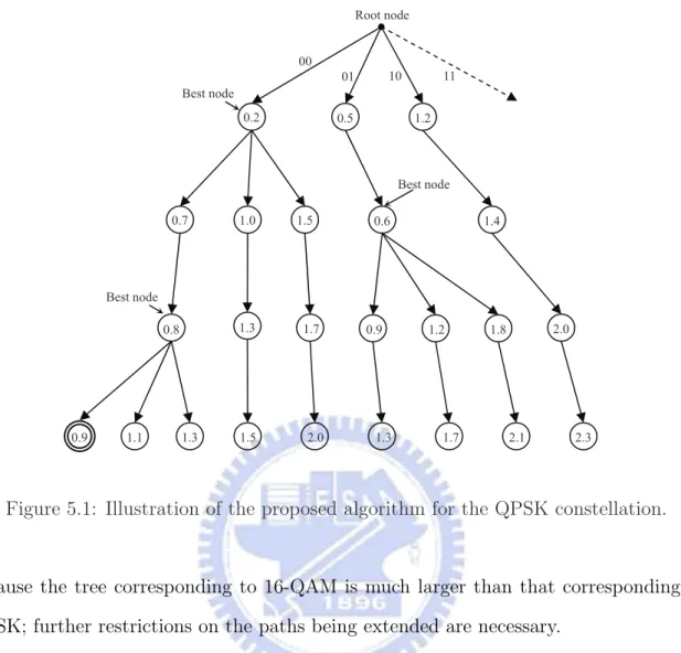
5.1 Illustration of the proposed algorithm for the QPSK constellation. . . 27
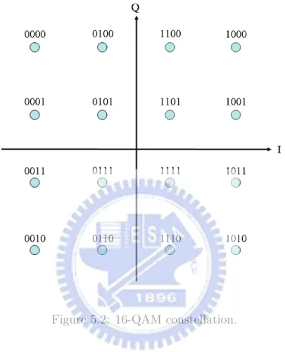
5.2 16-QAM constellation. . . 28
5.3 Illustration of the proposed algorithm for the 16-QAM constellation. . . . 29
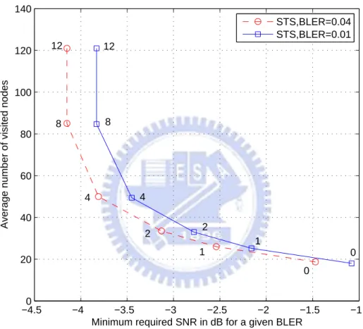
6.1 The LLR clipping under the single tree search (STS) strategy for the QPSK modulation. The numbers marked next to the nodes correspond to the used Lmax values. . . 31
6.2 The LLR clipping under the single tree search (STS) strategy for the 16-QAM modulation. The numbers marked next to the nodes correspond to the used Lmax values. . . 32
6.3 Comparisons of unsorted QRD, SQRD and MMSE-SQRD preprocessing applied to the STS for the QPSK modulation. The numbers marked next to the nodes correspond to the used Lmax values. . . 33
6.4 Comparisons of unsorted QRD, SQRD and MMSE-SQRD preprocessing applied to the STS for the 16-QAM modulation. The numbers marked next to the nodes correspond to the used Lmax values. . . 34
6.5 Impact of the run-time constraint on the STS SESD (with MMSE-SQRD preprocessing) for the QPSK modulation. The numbers marked next to the nodes correspond to the used Lmax values. . . 36
6.6 Impact of the run-time constraint on the STS SESD (with MMSE-SQRD preprocessing) for the 16-QAM modulation. The numbers marked next to the nodes correspond to the used Lmax values. . . 37
6.7 New tree traversal algorithm for the QPSK modulation. . . 38
Chapter 1
Introduction
In recent years, the wireless transmission with multiple antennas at the transmitter and receiver, also being referred to as multiple-input multiple output (MIMO) system [1] has attracted enormous interest. It is considered to be the technology that can provide significant capacity improvement over existing communication systems.
In an MIMO fading channels suffering additive white Gaussian noises (AWGN), dif-ferent data streams are transmitted from difdif-ferent transmit antenna elements via the same channel; so the receiver has to separate and recover these data streams. Some detection algorithms for MIMO systems have thus been proposed and are reviewed in the following. Linear detection methods, such as the zero-forcing (ZF) or minimum mean-squared error (MMSE) [2], estimate the information of channel matrix and then try to compensate the channel effect. The linear detection methods usually have low computational complexity, but they cannot totally remove the inter-stream interference and will induce noise enhancement. They accordingly may result in significant perfor-mance degradation. The brutal-force maximum likelihood (ML) detector [3] is optimal in terms of performance, but the computational complexity is very high because it is implemented based on exhaustive search. The sphere decoding (SD) algorithm [4], [5] can reduce the complexity of the ML detector and can still find the ML solution over the MIMO channel. Thus it has drawn quite a lot of research attention recently. The
during the codeword search.
In this thesis, we will focus on the SD algorithm and its tree search strategy. The strategy is generally based on the branch and bound (BB) notion [6], [7]. We will further classify different searching strategies and remark on their advantages and disadvantages. In particular, we will present the soft-output SD algorithm [8] and propose a tunable decoder (equivalently, a new tree search strategy) based on it, of which the performance can be made ranged between the hard-output successive interference cancelation (SIC) and the max-log a posteriori probability (APP) detection [9].
Note that in comparison with the hard-output SD algorithm, the soft-output SD algo-rithm generally requires much more computational complexity; so, a particular method to reduce the complexity of the soft-output SD algorithm [10] may be necessary. Some known methods of complexity reduction in the literature include log-likelihood ratio (LLR) clipping, channel matrix regularization, or imposing a constraint on the maxi-mum computational complexity of the decoder (i.e., run-time constraint). As expected, these methods reduce the decoding complexity at a price of the performance degrada-tion. We will then propose in this thesis a new tree search strategy that results in less performance degradation (i.e., better performance) and also less complexity than the methods mentioned above. This idea behind our proposed strategy is basically similar to that of the M-algorithm [11] and the fixed-complexity SD algorithm [12]. Detail will be given in later chapters.
The remaining parts of the thesis are organized as follows. In Chapter 2, we introduce the system model. In Chapter 3, we review some general MIMO detection methods as well as the BB algorithm based on sphere decoders. Chapter 4 gives a detailed descrip-tion of the soft-output SD algorithm and the existing methods to reduce its complexity. In Chapter 5, the idea for our proposed algorithm to reduce the computational com-plexity of the soft-output SD algorithm without much sacrifice of the performance is presented. Chapter 6 summarizes and remarks our simulation results. Finally, we draw
Chapter 2
System Model
We consider an MIMO communication system with NT transmit antennas and NR
receive antennas, where NT ≤ NR, as shown in Fig. 2.1.
T R,N N
h
,1 Nh
R T N 1,h
1,1h
Demux Data to substreams Modulation 1 X T N X 1y
R Ny
Transmitter Receiver Detector Estimated data Input data n1 R N nFigure 2.1: An MIMO system model.
At the transmitter end, Q coded information bits are mapped onto a complex con-stellation O, e.g., QPSK, 16-QAM, etc. Hence, the number of concon-stellation points is
|O| = 2Q. The set of transmitted system vectors is then ONT. We assume that the
channel suffers flat fading. The received symbol vector thus can be written as:
where
x = [x1, · · · , xNT]
T ∈ ONT (2.2)
is the transmitted symbol vector,
y = [y1, · · · , yNR]
T ∈ CNR (2.3)
is the received symbol vector,
n = [n1, · · · , nNR]
T ∈ CNR (2.4)
is the independent zero-mean Gaussian-distributed complex noise vector with common variance N0 per entry, and
H = h1,1 · · · h1,NT ... . .. ... hNR,1 · · · hNR,NT ∈ CNR×NT (2.5)
is the channel matrix. In the above expression, C denotes the domain of complex num-bers. We assume that the elements of channel matrix H are complex Gaussian variables with zero mean and unit variance and can be perfectly estimated by the receiver. In our setting, the average transmit symbol power of each antenna is also normalized to 1, i.e., x has a covariance matrix E{xxH} = σ2
xINT, where σ
2
x= 1 and INT is the NT × NT
Chapter 3
General Methods of MIMO
Detection and Decoder
In this chapter, we will introduce existing MIMO detection schemes to dates. Specifically, we will first survey two linear detectors, and then we will introduce the brutal-force maximum likelihood (ML) detector, followed by the ML sphere decoder.
3.1
Linear Detectors
The idea behind linear detectors is to use a multiplicative matrix to linearly combine the received symbol vector y in order to estimate the transmitted symbol vector x. Such an operation is apparently linear. In a mathematical form, the linear detectors determine a matrix W such that the estimator ˆx is given by ˆx = Wy. In the sequel, we will introduce two perhaps the most commonly used MIMO linear detectors, the Zero-Forcing (ZF) and Minimum-Mean-Square-Error (MMSE).
3.1.1
Zero Forcing Detector
Zero-Forcing detector removes the distortion due to the channel matrix H by applying its pseudo-inverse:
WZF= (HHH)−1HH. (3.1)
It is easy to verify that ˆ
thus, the estimator is perfect in absence of the additive noise n. The ZF detector is considered a simple detector since it only requires to compute the pseudo-inverse of the channel matrix. But it ignores the noise effect; hence, after being multiplied by WZF,
the noise n may be amplified and enhanced.
3.1.2
Minimum Mean Squared Error Detector
As its name reveals, the minimum mean square error detector determines its W by minimizing the mean square error, E{(Wy − x)(Wy − x)H}. Since it takes the additive
noise n into account, it has no noise enhancement problem like the ZF detector does. Solving minWE{(Wy − x)(Wy − x)H} subject to y = Hx + x, we obtain
WMMSE =
¡
HHH + N0I
¢−1
HH. (3.2) Similar to the ZF detecotr, the filter output WMMSEy will be detected to the nearest
constellation point in the sense of the Euclidean distance. Although superior in per-formance to the ZF detector, the MMSE detector requires additional knowledge of the noise power N0, which may not be available in certain applications.
3.2
Brutal Force Maximum Likelihood Detector
The maximum likelihood (ML) detector gives the estimate ˆx that maximizes the pos-teriori probability Pr(y|x, H). Since n is complex Gaussian distributed, we can derive that
ˆ
xML= arg min
x∈ONT k y − Hx k
2 . (3.3)
The brutal force ML detector then solves this minimization problem by exhaustively searching all possible symbol vectors. Although optimal in performance, the brutal force ML detector will result in an exponentially increasing decoding complexity with respect to the size of the system constellation ONT.
3.3
Sphere Decoding Algorithm
The sphere decoding (SD) algorithm has recently been used to solve the signal detec-tion problem for MIMO systems because it can significantly reduce the computadetec-tional complexity while maintaining the same performance as an ML detector.
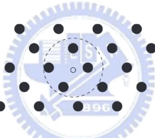
The idea behind the SD algorithm can be described as follows. It first sets a sphere centered at the received symbol vector with some properly chosen radius. Instead of searching the entire system constellation, it only searches the constellation points inside the sphere. We can then easily check from Fig. 3.1 that the constellation point that is closest to the received symbol vector must be located inside the sphere; hence, the optimality in performance remains after the introduction of the sphere.
Figure 3.1: Illustration of the sphere decoding algorithm.
The set of lattice points Hx lying inside a sphere centered at y with square radius r can be written as:1
r ≥k y − Hx k2 . (3.4)
It is in general difficult to find all NT-dimensional lattice points at once inside the sphere.
The SD algorithm achieves this goal through the help of a tree search. Specifically, it constructs a tree, in which the branch at the k-th level corresponds to the k-th dimension of the lattice points. It then locates those lattice points validating (3.4) in a
dimension-1In this thesis, r is used to denote the square radius rather than radius for the convenience of later
by-dimension fashion. The complexity of the SD algorithm thus depends on the size of the symbol constellation.
Next, we will divide the SD algorithm into two stages: 1) preprocessing stage and 2) tree search stage. The preprocessing stage is primarily concerned with the construction of the tree structure, while the tree search stage checks the validity of (3.4) based on the branch and bound (BB) algorithm.
3.3.1
The Preprocessing Stage
In order to facilitate the validation of (3.4) in later tree search stage, the channel matrix H is QR-decomposed [13] as H = Q · R 0(NR−NT)×NT ¸ (3.5) where the NR× NR matrix Q is unitary, and R is an NT × NT upper triangular matrix
with diagonals being real-valued. Multiplying (2.1) by QH leads to a modified
input-output relation as
˜
y = Rx + ˜n (3.6) where ˜y and ˜n respectively contain the first NT components of QHy and QHn. In
matrix form, the above equation can be written as ˜ y1 ... ˜ yNT = r1,1 r1,2 · · · r1,NT 0 r2,2 · · · r2,NT ... ... ... ... 0 · · · 0 rNT,NT x1 ... xNT + ˜ n1 ... ˜ nNT . (3.7) As Q is unitary, ˜n remains independent Gaussian distributed with zero mean and com-mon variance N0/2. Hence, (3.3) can be equivalently rewritten as
ˆ xML = arg min x∈ONT k ˜y − Rx k 2= arg min x∈ONT NT X i=1 ¯ ¯ ¯ ¯ ¯y˜i− NT X j=i ri,jxj ¯ ¯ ¯ ¯ ¯ 2 . (3.8) Define the partial symbol vector (PSV) as x(k) = [x , x , . . . , x ]T, and form
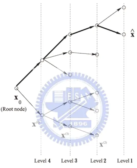
exemplified tree of four levels is illustrated in Fig. 3.2. Here, for convenience of its description, we count the levels of the tree from leaves to root. The nodes at level k are therefore marked by x(k). The dummy root note is conveniently marked as x
0.
Figure 3.2: The tree to be searched by the SD decoder. In this example, NT = 4.
Next, we define recursively the partial Euclidean distance (PED) d(x(k)) to be equal
to dk= dk(x(k)), where
and dNT+1 is initialized as 0, and the distance increment (DI) |ei| 2 is given by |ei|2 = ¯ ¯ ¯ ¯ ¯y˜i− NT X j=i ri,jxj ¯ ¯ ¯ ¯ ¯ 2 . (3.10)
It is then clear from the formulas that the PEDs only depend on the PSVs, and they can be regarded as the branch metrics during the tree search.
3.3.2
The Tree Search Stage
After preprocessing, the problem is transformed to the searching of the best path in a tree. A brutal force ML detector will visit all possible leaf nodes in order to find the leaf with the smallest metric value. However, visiting all leaf nodes will cost a large number of computations. The SD decoder then introduces the branch and bound (BB) algorithmic concept to reduced the number of nodes visited.
Before the presentation of the tree search process, we introduce some notations and terminologies used later.
• ACTIVE is a list of nodes that will be further explored.
• f (x(k)) ∈ R is a cost or metric function associated with node x(k) in the tree.
• t ∈ RNT×1 is a vector of which the component is the metric bound for each level.
• A node x(k) in the search space is a valid node if f (x(k)) < t
k.
• “sort” is a rule that sorts the nodes in the ACTIVE list.
• “gen” is a rule that decides which child node will be extended if there are more than one.
• g1 and g2 are rules used to tighten the bounding vector t.
• nc is a temporary variable that counts the number of nodes being visited or
ex-tended.
• The complexity of a tree search is measured as the number of nodes visited during the search.
• Two search algorithms or strategies are said to be equivalent if they visit the same set of nodes.
• A BB search algorithm that guarantees to find the leaf with the least metric is called an optimal BB search algorithm. If an algorithm does not guarantee the finding of the ML path, it is called a heurictic BB search algorithm.
With these notations and terminologies, a generic branch and bound (GBB) search algorithm can be described as follows.
GBB(f, t, sort, gen, g1, g2)
Step 1. Create an empty ACTIVE list. Place the root node in ACTIVE. Set nc← 0.
Step 2. Let x(k) be the current top node in ACTIVE.
If x(k) is a leaf node,
then set t ← g1(t, f (x(k))) and ˆx ← arg min(d(x(k)), d(ˆx)),2
and remove x(k) from ACTIVE, and go to Step 4.
If x(k) is not a valid node (i.e, f (x(k)) ≥ t
k)
or all valid child nodes of x(k) have already been generated,
then remove x(k) from ACTIVE, and go to Step 4.
Generate a valid child node x(k−1) of x(k), which has not been generated
before, according to the order given by gen, and place it in ACTIVE. Set nc= nc+ 1 and t ← g2(t, nc, ACTIVE).
2Here, if ˆx is null, meaning that ˆx has never been assigned, then d(ˆx) = ∞, and hence ˆx ←
Step 3. Sort the nodes in ACTIVE according to sort.
Step 4. If ACTIVE is empty, then stop the algorithm and output ˆx; else, go to Step 2.
In the following subsections, we will present three kinds of GBB algorithms to be used in the tree search [14] and remark on their characteristic.
3.3.2.1 Depth-First Search Algorithm
The GBB search algorithm will become depth-first search (DFS) in nature under the following condition. The sort rule will always put a node with the smallest level number
k on top of the ACTIVE list. Therefore, the DFS always forwards the search to the
next level (meaning to reduce the level k of the top node x(k)) except when a leaf node
is reached in which case the node in the previous level will be searched. 3.3.2.2 Breadth-First Search Algorithm
The breadth-first search (BrFS) is a tree traversal search rule that only forwards its search. In such case, the sort rule will always put a node with the largest level number
k on top of the ACTIVE list. The idea of the BrFS is to perform a full search in the
current level before forwarding to the next level. As a result, when the last level is reached, it can guarantee to output the ML solution.
3.3.2.3 Best-First Search Algorithm
The best-first search (BeSF) is also called the metric-first search. The idea of the BeSF is that all nodes in the ACTIVE list are sorted in ascending order of their cost function
f . Once a leaf node reaches the top of the ACTIVE list, the algorithm will reset t (via
function g1) to invalidate all other nodes in the list. As such, these remaining nodes will
be removed subsequently, and the only leaf node that has been the top node in ACTIVE will be outputted. It can be shown that when function f satisfies certain monotonicity
3.3.2.4 Analyses of the Tree Search Strategies
The three tree search strategies mentioned above can all be used to find the ML solution. The BrFS is similar to doing the exhaustive search if no bounding function is set to invalidate the nodes. The reduction of its complexity can perhaps be achieved by introducing an elaborate design of t, g1 and g2. Nevertheless, the BrFS has the highest
computational complexity among the three strategies.
The DFS is usually used with the notion of sphere radius update. In other words, when a leaf node is reached, the radius will be updated via g1. The radius is set to
be infinity initially and will be monotonically tightened during the tree search process. Through this, some nodes are invalidated and excluded from the search, and the com-plexity is reduced.
The BeFS is generally more efficient than the BrFS and DFS. It does not rely on the sphere radius node invalidation but simply chooses to extend the node with the lowest metric. In principle, the BeFS is the most favored when the complexity is concerned.
Chapter 4
Soft-Output Sphere Decoding and
Methods for Complexity Reduction
The SD algorithm introduced in Chapter 3 belongs to the class of hard-output decoders. The goal of the hard-output decoders is to find and directly output the ML solution. In this chapter, we will turn to the soft-output sphere decoder, which is the main focus of this thesis. Some methods to reduce the decoding complexity of the soft-output sphere decoders will also be introduced.
4.1
Soft-Output Sphere Decoding
The soft-output MIMO detection requires a soft output. Its purpose is to cooperate with an outer code in protecting the transmitted data. Hence, the soft-output sphere decoding needs to provide soft values to the outer code decoder. These soft output values specifically are the log-likelihood ratios (LLRs) of outer code bits. From this, we may infer that the soft-output SD algorithm is different from the hard-output SD algorithm mainly in that it examines not only the ML solution but also all other decoding possibilities so as to generates the LLRs.
4.1.1
Computation of the Max-Log LLRs
the max-log soft output in this thesis, which is an approximation to the true LLR. This max-log approximation [9] for bit xj,b can be written as
L(xj,b) = min
x∈Xj,b(0)
k y − Hx k2 − min
x∈Xj,b(1)
k y − Hx k2, (4.1)
where Xj,b(0) and Xj,b(1) are respectively the sets of symbol vectors that have the b-th bit in the j-th entry equal to 0 and 1.
It can be easily seen that one of the two minima in (4.1) is given by
λML=k y − HxMLk2, (4.2)
which is the metric associated with the ML solution xML. Denote the b-th bit in the
j-th entry of xML as xML
j,b ∈ {0, 1}, and let its binary complement be denoted by xMLj,b .
Then, the minimum, other than λML in (4.1), can be written as
λM L
j,b = min
x∈Xj,b(xMLj,b)
k y − Hx k2 . (4.3)
By combining (4.2) and (4.3), the max-log LLRs can be equivalently expressed as
L(xj,b) = λML− λM L j,b , if xMLj,b = 0; λM L j,b − λML, if xMLj,b = 1. (4.4) From (4.4), we conclude that the max-log APP MIMO detection can be realized via the determination of xML, λML and λM L
j,b for j = 1, 2, . . . , NT and b = 1, 2, . . . , Q.
4.1.2
Max-Log APP MIMO Detection via a Tree Search
We can transform the computations of (4.2) and (4.3) into a tree search problem and then use the SD algorithm to obtain the LLRs in (4.4) efficiently. Details are given below.
By employing the same idea of preprocessing mentioned in the previous chapter, the channel matrix H is QR-decomposed to H = QR; then, we multiply QH to both sides
of (2.1). After the preprocessing stage, the equivalent characterizations of λMLand λM L j,b
can be respectively obtained as
λML= min x∈ONT k ˜y − Rx k 2 (4.5) and λM Lj,b = min x∈Xj,b(xMLj,b) k ˜y − Rx k2 . (4.6) From (4.7), we see that the soft-output SD algorithm evidently needs to compute
λM L
j,b for every j and b, so it is anticipated to involve much more computational efforts
than the hard-output SD algorithm. In the sequel, we will introduce two tree traversal strategies, proposed in [15] and [16], for the generation of the LLR values. The first is referred to as repeated tree search (RTS) strategy [15], while the second is called the single tree search (STS) strategy [16]. The latter in general can save more computational complexity than the former.
4.1.2.1 Repeated Tree Search (RTS)
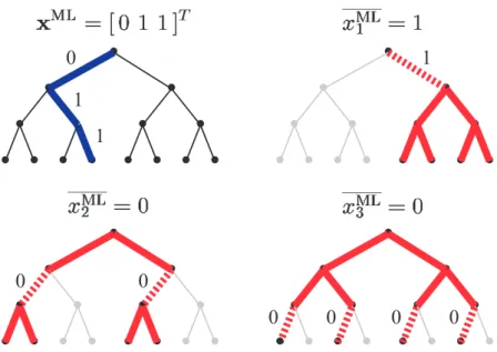
The idea behind the RTS strategy is to find the ML solution using the hard-output SD algorithm first; then, repeat the tree search in order to compute (4.7) for every bit in the symbol vector. It should be noted that during the repeated tree search for the computations of (4.7) for specific j and b, the nodes corresponding to xj,b = xMLj,b are
all excluded. This can save some amount of computational efforts. For example, for the BPSK constellation shown in Figure 4.1, where b is always equal to 1 and hence can be omitted, the tree for the computation of xML
1 excludes the left seven nodes
corresponding to x1 = xML1 = 0. Likewise, the tree for the computation of xML2 removes
six nodes corresponding to x2 = xML2 = 1. Then, the tree for the computation of xML3
eliminates the bottom four nodes corresponding to x3 = xML3 = 1.
” to refer to the node corresponding . Each path from the root down to a leaf . The solution of (6) and (7) corresponds to the leaf associated with the smallest , respectively. The basic building block underlying the two tree traversal strategies described in the next section is the Schnorr-Euchner (SE) sphere decoder (SESD) with radius reduction [15], [16], briefly summarized as follows: The search in the tree is constrained to nodes which and tree traversal is performed depth-first, visiting the children of a given node in ascending order of their PEDs. The basic idea of radius reduction is and to update the radius has been reached. This avoids the problem of choosing a suitable initial radius
0 1 1 1 0 0 0 0 0 0 !"# $%&'( !"# $%&'( ) *"+,%-'. /"0123456 789:9 ;<
Figure 4.1: BPSK-constellation in the RTS strategy.
• It may redundantly repeat some branch computations, which can be clearly seen from the three trees with red-colored branches in Figure 4.1.
• It involves a minimization operation over the subset X(xMLj,b)
j,b .
4.1.2.2 Single Tree Search (STS)
The STS is a more efficient tree search strategy when it is compared with the RTS. It ensures that every node in the tree is visited at most once. In particular, the STS searches for the ML solution and all counter-hypotheses concurrently (meaning, treating the ML solution as one of the hypotheses; so, xML
j,b is a counter-hypothesis), so it reduces
considerably the computational complexity.
The STS SD algorithm is initialized with λML= λM L
j,b = ∞ for every j and b. Then,
the tree search begins. When a leaf is reached, two situations will be considered:
• If a new ML hypothesis solution x is found, i.e., d(x) < λML, all λM L
j,b ’s, for which
updates:
λML ← d(x) and xML← x.
That is to say, the metric of the former ML hypothesis becomes the metric of a new counter-hypothesis. This procedure makes sure that at all times λM L
j,b is the
metric associated with a valid counter-hypothesis to the current ML hypotheses.
• In case d(x) ≥ λML, only the counter-hypotheses have to be checked. The rule
is as follows. For all j and b such that xj,b = xMLj,b and d(x) < λM Lj,b , the decoder
updates λM L
j,b ← d(x).
Since the STS is more efficient than the RTS, we will focus on the STS and only introduce the methods regarding its complexity reduction.
4.2
Methods for Complexity Reduction for the STS
So far, we have discussed the strategies that compute the exact LLR values and do not compromise on the performance. However, computing the exact LLR values will require a large amount of computational complexity. Thus, the goal in the section is to describe some methods to reduce the complexity with a trade-off on the performance (i.e., the LLR values obtained will be approximate rather than exact).
In this thesis, the complexity measure that we adopt is the number of nodes (including the leaves but excluding the root) visited by the decoder.
4.2.1
LLR Clipping
The soft LLR values are in general unbounded. In practice, we might need to con-straint the range of the LLR values to facilitate a fixed-point implementation. With the boundedness constraint, however, some performance degradation will be introduced.
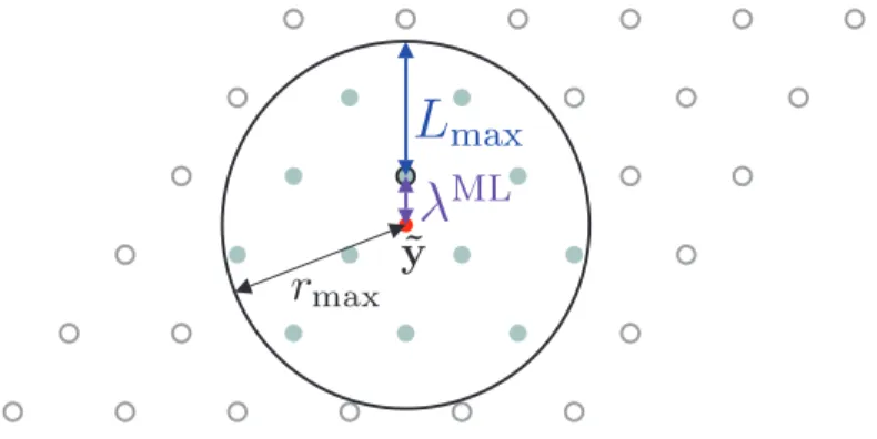
where Lmax is a chosen maximum LLR value. This is often called LLR clipping.
An operational interpretation of the LLR clipping is to restrict the search domain for lattice points inside the square radius rmax = λML+ Lmax as illustrated in Fig. 4.2.
Figure 4.2: LLR clipping restricting the square radius for lattice point search to rmax=
λML+ L max.
When a leaf is reached, the square radius will be updated according to
rj,b ← min{rj,b, λML+ Lmax}. (4.8)
This ensures that the resultant LLRs are bounded by Lmax. The LLR clipping can also
be done for each bit:
λM Lj,b ← min{λM Lj,b , λML+ Lmax}, ∀j, b. (4.9)
It can be anticipated that if Lmax = ∞, the LLR clipping returns the exact
max-log LLRs. In another extreme case where Lmax = 0, the LLR clipping results in a
informationless soft-output as (4.7) makes L(xj,b) = 0 for all j and b; hence, the decoder
can only report the hard output xML. So, by adjusting the L
max, we may reduce the
search complexity at a price of a less accurate soft output. From simulations, we observe that the performance of the soft output SD decoder degrades gracefully with respect to
Lmax. Therefore, the adjustment of the parameter Lmax may induce a good tradeoff in
4.2.2
Sorting and Regularization
This subsection introduces two techniques that take the effective signal-to-noise ratios of the system into consideration.
Sorting: Sorting is an effective method to reduce the complexity in sphere decoding
without compromising the performance. It performs the QR-decomposition on HP instead of H, where P is an NT × NT column permutation matrix. The idea behind
sorting is to let the diagonal entries of the upper triangular matrix R being sorted in ascending order such that the stronger streams in term of effective signal-to-noise (SNR) ratio (corresponding to tree levels) are closer to the root. In the following, we will refer to this method as sorted QR-decomposition (SQRD) [17].
Regularization: If the realization of channel matrix H is in a poor condition, it will
cause high search complexity due to the low effective SNR on some spatial streams. An efficient way to resolve this problem is to operate on a regularized channel matrix, i.e., to work on the sorted QR-decomposition on
· H
αINT
¸
P = QR, (4.10) where α is a suitably chosen regularization parameter, Q is an (NR+ NT) × NT unitary
matrix , R is an NT × NT upper triangular matrix and I denotes the NT × NT identity
matrix. We then partition Q to Q = [QT
1 QT2]T, where Q1 is of dimension NR× NT and
Q2 is of dimension NT × NT. This gives that
R = QH · H αINT ¸ P = £QH 1 QH2 ¤· H αINT ¸ P = ¡QH 1 H + αQH2 ¢ P (4.11)
The system model can then be equivalently transformed to ˜ y = QH 1 y = QH 1 Hx + QH1 n = QH1 Hx + αQH2 x − αQH2 x + QH1 n = ¡QH 1 H + αQH2 ¢ x − αQH 2 x + QH1 n = R˜x + ˜n, where ˜x = P−1x and ˜n = −αQH
2 x + QH1 n. The max-log LLRs in (4.1) can accordingly
be approximated by L(xj,b) ≈ min ˜ x∈Xj,b(0) k ˜y − R˜x k2 − min ˜ x∈Xj,b(1) k ˜y − R˜x k2 (4.12)
by pretending ˜n to be i.i.d. complex Gaussian distributed. Note that the effective noise-plus-(self)-interference (NPI) vector
˜
n = −αQH
2 x + QH1 n (4.13)
is neither i.i.d. nor complex Gaussian due to the self-interference term −αQH
2 x. That is
why (4.12) is simply an approximation to (4.1). In order to get a good approximation, we compute the covariance matrix of ˜n as
K = E[˜n˜nH] =¡RRH¢−1|α|2¡|α|2− N 0
¢
+ N0INT, (4.14)
where we assume E[xxH] = I
NT. Then, setting α = ±
√
N0 corresponds to an MMSE
regularization, yielding K = N0INT. This gives a theoretically conclusive aspect of
the so-called MMSE-SQRD [18] with the requirement that N0 needs to be estimated.
In the remainder of this thesis, the QR-decomposition in (4.10) with α = ±√N0 will
be employed whenever the MMSE-SQRD is referred to. We end the discussion on the MMSE-SQRD by pointing out that at the end of the decoding process, the LLRs obtained corresponding to ˜x need to be multiplied by the permutation matrix P to resume its order corresponding to x.
4.2.3
Run-Time Constraint
The computational complexity reduction methods discussed thus far depend on the channel statistics; hence, the decoder throughput varies with respect to the condition of the channel. Many practical applications however require a stable throughput. This leads to the run time constraint of the soft-output SD algorithm via setting a maximum number of nodes that the SD decoder is allowed to visit. In principle, the run-time constraint will prevent the system from achieving the max-log APP performance, so it is critical to find a way to minimize the performance degradation.
We will only consider the STS SD algorithm with run time constraint below. As previously mentioned, the run-time constraint will stop the tree search process when the number of visited nodes achieves the upper limit. The STS SD decoder will then return the ML solution and the LLRs that have been found so far.
In terms of the system aggregate throughput, we may consider the decoding of a sequence of N symbol vectors (of dimension NT). We suppose the maximum number
of tree nodes allowed to be visited for the decoding of this N-symbol-vector block to be denoted by N · Davg, where Davg is the average run time constraint. Then, the decoding
of the k-th symbol vector can, for example, be chosen according to the maximum-first (MF) scheduling strategy [19] as Dmax(k) = N · Davg− k−1 X i=1 D(i) − (N − k)NT (4.15)
nodes for k = 1, 2, . . . , N , where D(i) denotes the number of nodes actually visited during the decoding of the i-th symbol vector.
The idea behind (4.15) is that when a symbol vector is decoded, it is allowed to use all the remaining budget but has to maintain a safety margin (N − k)NT for the remaining
(N − k) symbol vectors. This margin allows the remaining symbols to achieve at least the hard-output SIC performance. Note that if Davg = NT, D(k) = Dmax(k) = NT;
if some of the LLRs have not yet been obtained at the end of the decoding process, they will be set to the ±Lmax.
Chapter 5
New Tree Traversal Strategy
In the previous chapter, some tunable MIMO detectors based on the soft-output sphere decoding algorithm with performance ranging from that of the hard-output successive interference cancellation (SIC) to that of the max-log APP detection are introduced. These tunable MIMO detectors provide a tradeoff between the detection complexity and performance. Along this research line, we want to find a new tree traversal strategy that yields almost the same computational complexity but has better performance. The tree traversal strategy that we newly proposed in this chapter is basically MMSE-SQRD-based and is a refinement of the Schnorr-Euchner sphere decoder (SESD) [20].
We will focus on the QPSK and 16-QAM constellation using Gray mapping. Since the original proposed method that improves the performance for the QPSK constellation results in very limited improvement when it is applied to the 16-QAM, a different tree search method will be proposed for the 16-QAM. The two methods respectively for the QPSK and 16-QAM will then be introduced in two separate sections.
5.1
New Tree Search Strategy for QPSK
The key of our tree search strategy is that only the paths that generate the LLR values will be extended. This can be done based on two observations. First, since a QPSK symbol only carries two information bits, once the best path at the current level is
of the SESD. In other words, the required counter-hypotheses for the computations of the LLRs are guaranteed to be included in these three extended paths. Secondly, we observe that for the paths other than the best path at the current level, only the best successor path needs to be extended. This process will be repeated in every level.
For clarity, we summarize the proposed algorithm used in the QPSK constellation in Table 5.1:
Step 1 : Start from the root node and set nc← 0.
Step 2 : Expend the top three paths originated from the root node. Set nc= nc+ 3 and k = NT.
Step 3 : At the k-th level:
Expend the top three successor paths of the best path and set nc= nc+ 3.
Extend the best successor path of the remaining paths and set nc= nc+ 1.
Set k = k − 1.
Step 4 : Sort the extended paths ending at the k-th level in ascending order of their metrics.
Step 5 : If k = 1, use all extended paths ending at this level to generate the LLR values;
else go to Step 3.
Table 5.1: New Tree Search Algorithm for the QPSK constellation.
An example is illustrated in Fig. 5.1 for a better understanding of our proposed method.
5.2
New Tree Search Strategy for 16-QAM using
Gray Code Mapping
In the 16-QAM constellation, an extension tree search strategy from the simple one for QPSK, which we just introduced, does not provide a visible performance improvement
0.2 Best node Root node 0.5 1.2 0.7 1.0 1.5 0.6 1.4 0.8 1.3 1.7 0.9 1.2 1.8 2.0 1.1 1.3 11 10 01 00 Best node Best node 1.5 2.0 1.3 1.7 2.1 2.3 0.9
Figure 5.1: Illustration of the proposed algorithm for the QPSK constellation.
because the tree corresponding to 16-QAM is much larger than that corresponding to QPSK; further restrictions on the paths being extended are necessary.
The basic idea behind our proposal for 16-QAM follows similarly to the RTS. We will first find the ML solution by using the SESD algorithm with radius reduction [20]. Then, we can follow the ML path to decide which paths are relevant to the LLR computations and hence need to be extended. Since a 16-QAM symbol carries four information bits, only four successor paths corresponding to the counter-hypotheses of these four informa-tion bits (as contrary to the ML path) need to be extended in addiinforma-tion to the expansion of the ML path itself. For example, if 0000 corresponds to the ML symbol, then we will expand the paths corresponding to symbols 0001 and 0011, 0100 and 1100.1 Among the
1From Fig. 5.2, it can be observed that among the eight symbols of the form, 0xxx (i.e.,
{0000, 0001, 0010, 0011, 0100, 0101, 0110, 0111}), 0001 is apparently the closest to 0000. Similarly, 0011 should be the closest to 0000 among 0010, 0011, 0110, 0111, 1010, 1011, 1110, 1111. We can similarly
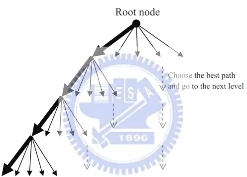
four paths that include all the counter-hypotheses corresponding to the ML symbol, the best path will be further extended. Further extension along this path only includes the best path. A simple illustration of the algorithm is given in Fig. 5.3.
Root node
Choose the best path and go to the next level
Chapter 6
Simulation Results
In this chapter, the flat fading MIMO channels with NT = 4 transmit antennas and
NR = 4 receive antennas are considered in all simulations. It is assumed that the
channel matrix H is perfectly known to the receiver. We assume additionally that the outer code that requires a soft output from inner modulation is a turbo code with rate
R = 1/2. The codeword lengths for the QPSK and 16-QAM constellations are 1000 bits
and 2000 bits, respectively, such that 500 symbols are transmitted for both cases.
6.1
Effect of LLR Clipping
As have been discussed in the previous chapter, the value of LLR clipping parameter Lmax
can be used to tune the performance from the exact max-log APP SESD (when Lmax=
∞) to the hard-output SESD (when Lmax = 0). We then simulate the complexities
versus the required SNRs to achieve a given block error rate (BLER) for the STS-based max-log APP SESD under different Lmax values. The results are summarized in
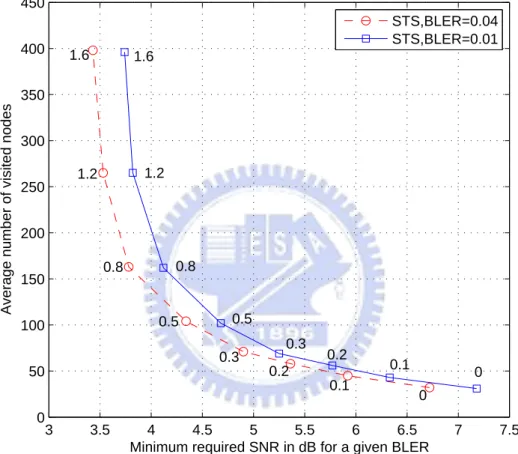
Figs. 6.1 and 6.2. We observe that the required SNRs decrease as Lmaxgrows at the price
of larger complexities. We also notice that when Lmax reaches 8 and 1.6 respectively
for the QPSK and 16-QAM, the system performance will achieve near-exact max-log APP performance. Based on these results, the LLR clipping level Lmax can be used to
−4.50 −4 −3.5 −3 −2.5 −2 −1.5 −1 20 40 60 80 100 120 140 0 1 2 4 8 12 0 1 2 4 8 12
Minimum required SNR in dB for a given BLER
Average number of visited nodes
STS,BLER=0.04 STS,BLER=0.01
Figure 6.1: The LLR clipping under the single tree search (STS) strategy for the QPSK modulation. The numbers marked next to the nodes correspond to the used Lmax values.
3 3.5 4 4.5 5 5.5 6 6.5 7 7.5 0 50 100 150 200 250 300 350 400 450 0 0.1 0.2 0.3 0.5 0.8 1.2 1.6 0 0.1 0.2 0.3 0.5 0.8 1.2 1.6
Minimum required SNR in dB for a given BLER
Average number of visited nodes
STS,BLER=0.04 STS,BLER=0.01
Figure 6.2: The LLR clipping under the single tree search (STS) strategy for the 16-QAM modulation. The numbers marked next to the nodes correspond to the used Lmax
6.2
Effect of Sorting and Regularization
Figs. 6.3 and 6.4 compare the impact of sorting and regularization on the complex-ity/performance trade-off of the STS algorithm. Specifically, these curves respectively correspond to standard (unsorted) QRD, SQRD and MMSE-SQRD at a target BLER of 0.01. We can see from the two figures that sorting and regularization can provide consid-erable reduction in complexity without sacrifice in performance, and the SQRD-MMSE can save almost half of the complexities.
−40 −3.5 −3 −2.5 −2 −1.5 −1 20 40 60 80 100 120 140 0 1 2 4 8 12
Minimum required SNR in dB for BLER=0.01
Average number of visited nodes
unsorted QRD SQRD MMSESQRD
Figure 6.3: Comparisons of unsorted QRD, SQRD and MMSE-SQRD preprocessing applied to the STS for the QPSK modulation. The numbers marked next to the nodes correspond to the used Lmax values.
3.5 4 4.5 5 5.5 6 6.5 7 7.5 0 50 100 150 200 250 300 350 400 450 0 0.1 0.2 0.3 0.5 0.8 1.2 1.6
Minimum required SNR in dB for BLER=0.01
Average number of visited nodes
unsorted QRD SQRD
MMSE−SQRD
Figure 6.4: Comparisons of unsorted QRD, SQRD and MMSE-SQRD preprocessing applied to the STS for the 16-QAM modulation. The numbers marked next to the nodes correspond to the used Lmax values.
6.3
Effect of Run-time Constraints
In Figs. 6.5 and 6.6, we illustrate the impact of imposing a run-time constraint according to a given N · Davg for a block of N = 125 symbol vectors. Three observations can be
made here:
• For a small Lmaxclipping level, the performance is dominated more by the clipping
rather than by the runtime constraint. For example, Fig. 6.5 shows that to enlarge
Davg from 16 to 256 does not improve the performance much when Lmax= 2.
• For a large Lmax clipping level, the algorithm will yield a high average search
complexity as anticipated. However, the performance remains poor unless we have sufficiently large Davg. For example, setting Lmax= 8 will introduce two apparent
performance groups for the Davg values simulated (i.e., {16, 24, 32} and {64, 128}),
and there is a sudden performance improvement when Davg increases beyond 64.
• For a given run-time constraint, there seemingly exists an optimal LLR clipping level Lmax(for example, Lmax= 8 for the curve corresponding to Davg = 64), which
minimizes the required SNR to achieve a target BLER. It is therefore important to choose the appropriate LLR clipping level in accordance with the average run-time constraint.
−4 −3.5 −3 −2.5 −2 −1.5 −1 −0.5 0 10 20 30 40 50 60 70 80 90 100 4 6 8 12 10 5 6 8 2 3 4 6 8 2 4 6 8
Minimum required SNR in dB for BLER=0.01
Average number of visited nodes
Davg = 128 Davg = 64 Davg = 32 Davg = 24 Davg = 16
Figure 6.5: Impact of the run-time constraint on the STS SESD (with MMSE-SQRD preprocessing) for the QPSK modulation. The numbers marked next to the nodes correspond to the used Lmax values.
3 4 5 6 7 8 9 10 11 0 20 40 60 80 100 120 140 160 180 0.1 0.2 0.3 0.5 0.8 1.2 1.2 0.8 1.2 0.3 0.5 0.8 1.2 0.1 0.2 0.3 0.5 0.8 1.2
Minimum required SNR in dB for BLER=0.01
Average number of visited nodes
Davg = 256 Davg = 128 Davg = 64 Davg = 32 Davg = 16
Figure 6.6: Impact of the run-time constraint on the STS SESD (with MMSE-SQRD preprocessing) for the 16-QAM modulation. The numbers marked next to the nodes correspond to the used Lmax values.
6.4
Effect of the New Tree Traversal Strategy
We now examine the improvement of our new tree traversal strategy. As shown in Fig. 6.7, the new algorithm can provide around 0.5 dB performance improvement than the MMSE-SQRD. As for the 16-QAM modulation illustrated in Fig. 6.8, 0.4 dB per-formance improvement can be resulted when the MMSE-SQRD is enhanced with our proposed method. −4 −3.5 −3 −2.5 −2 −1.5 −1 −0.5 0 10 20 30 40 50 60 70 80 90 100 4 6 8 12 10 5 6 8 2 3 4 6 8 2 4 6 8
Minimum required SNR in dB for BLER=0.01
Average number of visited nodes
Davg = 128 Davg = 64 Davg = 32 Davg = 24 Davg = 16 New Algorithm
3 4 5 6 7 8 9 10 11 0 20 40 60 80 100 120 140 160 180 0.1 0.2 0.3 0.5 0.8 1.2 1.2 0.8 1.2 0.3 0.5 0.8 1.2 0.1 0.2 0.3 0.5 0.81.2
Minimum required SNR in dB for BLER=0.01
Average number of visited nodes
Davg = 256 Davg = 128 Davg = 64 Davg = 32 Davg = 16 New Algorithm
Chapter 7
Conclusion and Future work
The purpose of this thesis is to present a new algorithm for soft detection in an MIMO system as a support to an outer code.
The existing results in sphere decoding have proven that it is a suitable technique for soft-output MIMO detection with a tunable complexity/performance trade-off. Such an adjustment in complexity/performance trade-off can be achieved by varying the LLR clipping level as well as the run time constraint. At this background, this thesis provides an additional enhancement based on an accurate counter-hypothesis analysis on the modulation constellation. Although a visible improvement has been obtained by our proposed method, further improvement can be possibly achieved if a more accurate counter-hypothesis analysis is given.
At the current stage, we only deal with the QPSK and 16-QAM modulations. Our experience shows that the method designed for the QPSK modulation may not be straightforwardly extendable to the 16-QAM modulation. It is possible that the same phenomenon will be observed when one tries to extend our method for the 16-QAM mod-ulation to a higher-QAM modmod-ulation. Hence, it should be interesting to see whether there exists a systematical method that can be extendably applied to to all, e.g., square QAM modulations.
Bibliography
[1] E. Biglieri, R. Calderbank, A. Constantinides, A. Goldsmith, A. Paulraj and H. V. Poor, MIMO wireless communications, Cambridge University Press, 2007.
[2] S. Verd´u, Multiuser Detection. Cambridge University Press, 1998.
[3] W. van Etten, ”Maximum likelihood receiver for multiple channel transmission sys-tems,” IEEE Trans. Commun., vol. 24, no. 2, pp. 276V283, Feb. 1976.
[4] C. P. Schnorr and M. Euchner, ”Lattice basis reduction: Improved practical algo-rithms and solving subset sum problems,” Math. Programming, vol. 66, no. 2, pp. 181V191, Sept. 1994.
[5] U. Fincke and M. Pohst, ”Improved methods for calculating vectors of short length in a lattice, including a complexity analysis.” Mathematics of Computation, vol. 44, pp. 463V471, Apr. 1985.
[6] E. L. Lawler and D. W. Wood, ”Branch-and-bound methods: A survey,” Oper. Res., vol. 14, pp. 699-719, 1966.
[7] J. Luo, K. R. Pattipati, P.Willett, and G. M. Levchuk, ”Fast optimal and subopti-mal any-time algorithms forCDMAmultiuser detection based on branch and bound,”
IEEE Trans. Commun., vol. 52, no. 4, pp. 632V642, Apr. 2004.
[9] B. M. Hochwald and S. ten Brink, ”Achieving near-capacity on a multiple-antenna channel,” IEEE Transactions on Communications, vol. 51, no. 3, pp. 389V399, Mar. 2003.
[10] R.Wang and G. Giannakis, ”Approaching MIMO channel capacity with reduced-complexity soft sphere decoding,” in Proc. of IEEE Wireless Communications and
Networking Conf. (WCNC), vol. 3, Mar. 2004, pp. 1620V1625.
[11] J. B. Anderson and S. Mohan, ”Sequential coding algorithms: A survey and cost analysis,” IEEE Trans. Commun., vol. COM-32, no. 2, pp. 169V176, Feb. 1984.
[12] L. G. Barbero and J. S. Thompson, ”A Fixed-Complexity MIMO Detector Based on the Complex Sphere Decoder,” in IEEE Workshop on Signal Processing Advances
for Wireless Communications (SPAWC 06), Cannes, France, July 2006.
[13] D. W¨ubben, R. B¨ohnke, J. Rinas, V. K¨uhn, and K. Kammeyer, ”Efficient Algorithm for Decoding Layered Space-Time Codes,” IEE Electronics Letters, vol. 37, no. 22, pp. 1348V1350, Oct. 2001.
[14] J. Anderson and S. Mohan, ”Sequential coding algorithms: A survey and cost analysis,” Communications, IEEE Transactions on [legacy, pre - 1988], vol. 32, no. 2, pp. 169V176, Feb 1984.
[15] R.Wang and G. Giannakis, ”Approaching MIMO channel capacity with reduced-complexity soft sphere decoding,” in Proc. of IEEE Wireless Communications and
Networking Conf. (WCNC), vol. 3, Mar. 2004, pp. 1620V1625.
[16] J. Jalden and B. Ottersten, ”Parallel implementation of a soft output sphere de-coder,” in Proceedings Asilomar Conference on Signals, Systems and Computers, Nov. 2005, pp. 581V585.
[17] D. Wubben, R. Bohnke, J. Rinas, V. Kuhn, and K. Kammeyer, ”Efficient algorithm for decoding layered space-time codes,” IEE Electronics Letters, vol. 37, no. 22, pp. 1348V1350, Oct. 2001.
[18] D. Wubben, R. Bohnke, V. Kuhn, and K. Kammeyer, ”MMSE extension of V-BLAST based on sorted QR decomposition,” in IEEE Proc. Vehicular Technology
Conference (Fall), vol. 1, Oct. 2003, pp. 508V512.
[19] A. Burg, M. Borgmann, M. Wenk, C. Studer, and H. Bolcskei, ”Advanced receiver algorithms for MIMO wireless communications,” in Proceedings of the Design
Au-tomation and Test Europe Conf. (DATE), vol. 1, May 2006, pp. 593V598.
[20] E. Agrell, T. Eriksson, A. Vardy, and K. Zeger, Closest point search in lattices, IEEE Transactions on Information Theory, vol. 48, no. 8, pp. 2201V2214, Aug. 2002.