基於幾何人臉特徵之智慧型頭部姿態估測

國 立 交 通 大 學

電控工程研究所

碩

士

論

文

基於幾何人臉特徵之智慧型頭部姿態估測

Intelligent Head Attitude Estimation based on Geometric

Facial Features

研 究 生：王宣竣

指導教授：陳永平 教授

基於幾何人臉特徵之智慧型頭部姿態估測

Intelligent Head Attitude Estimation based on Geometric

Facial Features

研 究 生：王宣竣 Student： Syuan-Jyun Wang

指導教授：陳永平 Advisor：

Professor Yon-Ping Chen

國 立 交 通 大 學

電控工程研究所

碩 士 論 文

A Thesis

Submitted to Institute of Electrical Control Engineering

College of Electrical and Computer Engineering

National Chiao Tung University

In Partial Fulfillment of the Requirements

For the degree of Master

In

Electrical Control Engineering

June 2013

Hsinchu, Taiwan, Republic of China

i

基於幾何人臉特徵之智慧型頭部姿態估測

學生：王宣竣 指導教授：陳 永 平 博士 國立交通大學電控工程研究所 摘要 Chines 近年來臉部特徵偵測和人臉辨識已被廣泛地研究,許多利用臉部特徵偵測的 應用也隨之發展。本篇論文即利用幾何人臉特徵，針對頭部姿態的方向和角度， 提出智慧型頭部姿態估測系統之設計。此系統能夠自動偵測影像中的人臉特徵， 包括眼睛及嘴巴,進而判斷頭部姿態的方向和角度。本系統分成三個步驟完成智 慧型頭部姿態估測系統設計,首先，利用膚色找出臉部位置後，使用幾何人臉特 徵達到眼睛及嘴巴的高偵測率，第二，製作頭部姿態的人臉模擬立體模型，可調 整臉部轉向角度及頭部傾斜角度，在轉盤上標有七個偵測點，根據不同的及 ，製作臉部模擬影像，並記錄每張影像的七個偵測點，作為類神經網路學習之 用，第三，經由監督式學習的類神經網路設計達到頭部姿態的估測。本論文所提 出的智慧型頭部姿態估測在於特定範圍內正確率可達 97.3%。

ii

Intelligent Head Attitude Estimation based on Geometric

Facial Features

Student:

Syuan-Jyun Wang

Advisor: Dr. Yon-Ping Chen

Institute of Electrical Control Engineering

National Chiao Tung University

ABSTRACT

Recently, facial feature detection and face recognition have been studied

extensively and many applications using facial feature detection have been developed.

This thesis is aimed at the development of head attitude estimation system (HAES)

based on geometric facial features to detect the face orientation and angle. The HAES

automatically detects eyes and mouth in the image as the facial features, and then

determine the head attitude. There are three steps to complete the intelligent head

attitude estimation. First, detect the human face based on skin color and use the

geometric facial features to the detection of eyes and mouth in high accuracy rate.

Second, build up a stereo facial model to simulate the head attitude which is able to

adjust the face orientation and angle by seven detecting points marked on the face

model. Record the seven detecting points on each image referring to a specific face

orientation and angle, which will be used in neural network learning. Third, the HAES

is completed by intelligent neural networks under supervised learning. The proposed

iii

Acknowledgement

誠摯感謝指導教授 陳永平老師在這兩年中的悉心指導與教誨，老師嚴謹的 治學態度，理論與實務並重的訓練，使得本論文得以順利完成。除了學術上的指 導，在待人處事方面的啟發更讓我獲益良多，這份師恩會令我永生難忘。同時也 感謝口試委員 林昇甫教授 張浚林教授對本論文所提出的珍貴意見與指證，讓本 論文能更加的完整。 除此之外，感謝可變結構控制實驗室的世宏學長平日在攻讀博士學位之餘， 不吝傳授知識與經驗及給予指導。此外，學長澤翰、文俊、文榜、榮哲、崇賢、 孫齊與振方，同學兆村、仕政、咨瑋與谷穎，學弟妹仁傑、惠琪、御旻與冠銘在 課業與研究上一起學習與勉勵，以及實驗室上的協助，感謝妳們在生活中帶給我 許多歡笑，使我兩年的研究所生活更加多采多姿。 最後，更要感謝我的父親、母親、大姊、小妹，你們的關心與鼓勵，給了我 許多的溫暖，由於你們的支持，使我能專心在學習領域上衝刺，最後再次由衷的 謝謝所有支持、關心與幫助過我的人。 謹以此篇論文獻給所有關心我、照顧我的人，你們的恩惠我銘感於心，由衷 感謝你們。 王宣竣 2013 .6

iv

Contents

Chinese Abstract……….………..………..…………..………...i English Abstract...…....…..………...…...ii Contents ..………….………..………..iii List of Figures………..………...……….……..….…….vi List of Tables……...………...………...….…viii Chapter 1 Introduction ...1 1.1 Preliminary ... 1 1.2 System Overview ... 2

Chapter 2 Related Works ...4

2.1 Introduction to ANNs ... 4

2.2 Back-Propagation Network ... 7

2.3 Skin Color Detection ... 10

2.4 Edge Detection ... 11

2.5 Morphology Operation... 12

Chapter 3 Head Attitude Estimation System ... 14

3.1 Facial Features Detection ... 14

3.1.1 Human Face Detection ... 14

3.1.2 Morphology Operation... 18

3.1.3 Connected Components Labeling ... 20

v

3.1.5 Facial Feature Detection ... 25

3.2 Geometric Facial Features ... 30

3.3 Head Attitude Estimation System Design ... 31

Chapter 4 Experiment Results ...38

4.1 Facial Features Detection ... 38

4.2 Geometric Facial Features... 40

4.3 Head Attitude Estimation System Design ... 42

Chapter 5 Conclusion and Future Works ...54

vi

List of Figures

Figure 1.2.1 Architecture of head attitude estimation ... 3

Figure. 2.1 Basic structure of a neuron ... 4

Figure. 2.2 Multilayer feed-forward network ... 6

Figure. 2.3 Neural network with one hidden layer ... 8

Figure. 2.4 Example of dilation ... 12

Figure. 2.5 Example of erosion ... 13

Figure 3.1.1.1 statistic range of skin ... 16

Figure 3.1.1.2 (a) Color image, (b) thresholded image using Eqs.(3.1.1)-(3.1.6) ... 17

Figure. 3.1.2.1 (a) Structuring element B (b) Structuring element C ... 18

Figure. 3.1.2.2 Steps for morphology operations (a) Initial image (b) Result of erosion using structuring element B (c) Result of dilation using structuring element C ...19

Figure. 3.1.3.1 Scanning the image ... 20

Figure. 3.1.3.1 Example of 4-pixel connected CCL ... 21

Figure 3.1.4.1 The proportion of the human face’s width and height ... 22

Figure 3.1.4.2 The flow chart of the human face detection ...23

Figure 3.1.4.3 To show real human faces detection of per step from the flow chart .24 Figure 3.1.4.1 Extraction the ROI of human face get the edge detection (a) shows original image (b) get ROI of human face (c) edge detection of human face. ...26

Figure 3.1.4.2 Head geometry ... 29

Figure 3.1.4.3 Head geometry divided to three part ... 29

vii

Figure3.3.2 Train vectors on human face ...31

Figure3.3.2 Train vectors on human face ...33

Figure3.3.3 Neural network structure for β angle of the human head geometric .... 33

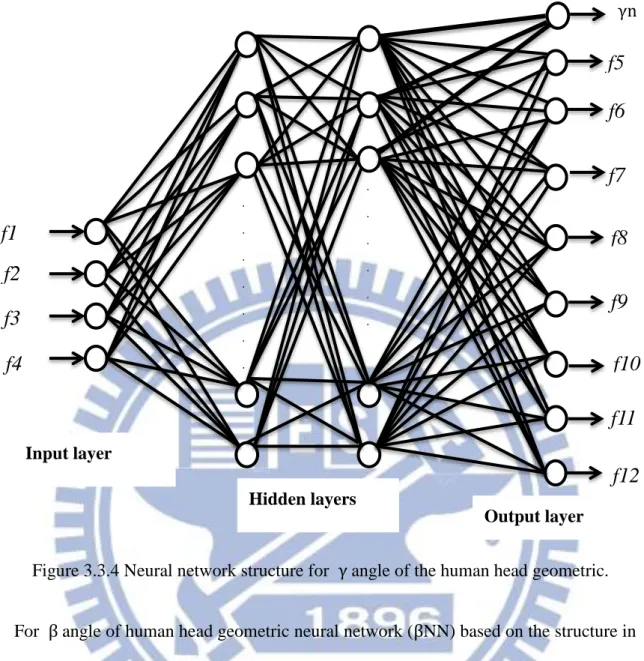
Figure 3.3.4 Neural network structure for γ angle of the human head geometric .... 34

Figure.3.3.5 linear transfer function ... 36

Figure.3.3.6 βNN ...36

Figure.3.3.7 γ NN ...37

Figure 4.1.1 The result of different people facial detection ...38

Figure 4.1.1 The result of different people facial detection ... 39

Figure 4.2.1 The turntable appearance ... 40

Figure 4.2.2 RGB color label seven points ... 41

Figure 4.2.3 Detection RGB colors ... 41

Figure 4.3.1 The different distance between webcam and stereo facial model. ... 47

Figure 4.3.2 A histogram relates to accuracy rate and angle-scale of βNN in case1 48 Figure 4.3.3 In different angle-scale curves, βNN relates to accuracy rate and distance in case 1 ... 49

Figure 4.3.4 A histogram relates to accuracy rate and angle-scale of βNN in case2 ... 50

Figure 4.3.5 In different angle-scale curves, βNN relates to accuracy rate and distance in case2 ... 51

Figure 4.3.6 A histogram relates to accuracy rate and angle-scales of γNN ... 52

Figure 4.3.7 In different angle-scale curves, γNN relates to accuracy rate and distance ... 53

viii

List of Tables

Table 3.1 Two angle of human head geometric………31

Table 4.1 Accuracy rate of three facial features detection………....38

Table 4.2 30CM distance of βNN off-line training parameter.………...43

Table 4.3 γNN off-line training parameter………...44

Table 4.4 All distance range of βNN off-line training parameter………45

Table 4.5 the βNN accuracy rate relating to angle-scale and distance in case 1….47 Table 4.6 the βNN accuracy rate relating to angle-scale and distance in case2…..49

1

Chapter 1

Introduction

1.1 Preliminary

Facial feature detection and face recognition have been studied extensively in last

decade and many applications used to detect facial features have been developed.

Several approaches have been proposed in the literature for facial feature detection

in front-view head images. Yuille, et al. [1] use deformable templates to search for the

facial features around the peaks and valleys of the intensity image. A similar approach

is used by Hallinan [2] to detect the eyes in an image. Ahmed Fadzil and Abu Baker [3]

adopt a multi-layered neural network to search the head area and locate the eyes. Chang

and Huang [4] and Ohya, et.al.[5] employ skin color to locate facial features in colored

images.

This thesis uses the methods proposed from Huang and Ohya, which are based on

skin color to detect facial features such as eyes and mouth and can achieve high

accuracy rate. According to the locations of eyes and mouth, which form geometric

facial features, we can develop the head attitude estimation system (HAES) which

determines the face orientation and angle as the head attitude.

Recently, in many researches the neural network has been carried out to deal with

problems of system modeling concerning nonlinearities and uncertainties. It is well

known that the neural network possesses excellent learning and mapping ability for

nonlinear system modeling and the most prevalent neural network architecture is based

on the back-propagation technique. Since the geometric facial features are nonlinear

and complex, in order to determine the face orientation and angle, the proposed HAES

in this thesis chooses the neural network with back-propagation algorithm to learn the

2

In the thesis, a stereo facial model is built up to simulate the head attitude which

includes seven points to represent the on geometric facial features. Three points are the

mouth and two eyes, and the other four points M1, M2, M3 and M4 construct a

rectangle to mask the face. The stereo facial model includes a human face image and

two angle-scaled turntables to indicate the facial angle γ and orientation β. To achieve the head attitude features, the left-eye is assigned as the original point. Then, choose

the difference of the right-eye to the original point as the vector V1 and the difference

of the mouth to the original point as the vector V2. Both V1 and V2 are adopted as the

neural network inputs. Similarly, the differences of the M1, M2, M3 and M4 to the

original point are set to be the vectors V3, V4, V5 and V6, respectively. Based on the

neural network back-propagation algorithm with inputs V1 and outputs V2, V3, V4,

V5, V6, β, and γ, the HAES is implemented. Most importantly, the HAES achieves a high accuracy rate up to 97.3% in the detection of face orientation and angle.

1.2 System Overview

In this thesis, a system is proposed for head attitude estimation (HAES). For

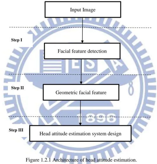
software architecture, the image shown in Figure 1.2.1 is the flow chart of the proposed

system.

There are three steps to complete the intelligent head attitude estimation, First,

detect the human face based on skin color and use the geometric facial features to the

detection of eyes and mouth in high accuracy rate. Second, build up a stereo facial

model to simulate the head attitude which is able to adjust the face orientation and angle

by seven detecting points marked on the face model. Record the seven detecting points

on each image referring to a specific face orientation and angle, which will be used in

3

under supervised learning. The remainder of this thesis is organized as follows. Chapter

2 describes the related works of the system. Chapter 3 describes intelligent head attitude

estimation based on geometric facial features system. Chapter 4 shows the experiment

results. Chapter 5 is the conclusions of the thesis and the future works.

Figure 1.2.1 Architecture of head attitude estimation.

Input Image

Facial feature detection

Geometric facial feature

Head attitude estimation system design Step I

Step II

4

Chapter 2

Related Work

2.1 Introduction to ANNs

The human nervous system consists of a large amount of neurons, including

somas, axons, dendrites and synapses. Each neuron is capable of receiving, processing,

and passing signals from one to another. To mimic the characteristics of the human

nervous system, recently investigators have developed an intelligent algorithm, called

artificial neural networks (ANNs). In the artificial intelligence field, ANNs have been

applied successfully to speech recognition, image analysis and adaptive control. This

thesis will apply ANNs to the face detection in an eyeball system through learning.

Figure. 2.1 Basic structure of a neuron.

w1 w2 w3 wn b x2 x3 xn x1 y

f(

)

5

Figure. 2.1 shows the basic structure of a neuron, whose input-output relationship

is described as 1 n i i i y f w x b     _  _ 



 (2.1)

where 𝑤_𝑖 is the weight at the input 𝑥_𝑖 and b represents the bias. The activation function f() can be linear or nonlinear, such as linear function, log-sigmoid function and tan-sigmoid function, respectively expressed as below:

(1) linear function ( ) f x x (2.2) (2) log-sigmoid function 1 ( ) 1 x f x e   (2.3) (3) tan-sigmoid function ( ) x x x x e e f x e e      (2.4)

Here, each input xi is multiplied by a corresponding weight wi, analogous to synaptic

strengths. The weighted inputs are summed to determine the activation level of the

neuron.

A general multilayer feed-forward network is composed of one input layer, one

output layer, and some hidden layers. For example, Figure. 2.2 shows a neural network

with one input layer, one output layer, and two hidden layers. Each layer is formed by

neurons with basic structure depicted in Figure. 2.1. The input layer receives signals

and response from the outside world, and then through the hidden layer to the output

layer, the response of the net can be read. Note that in some cases only the input layer

and output layer are required and the hidden layer can be omitted, i.e., the hidden layer

6

Compared with networks using single hidden layer, networks with multi-hidden

layer can solve more complicated problems. However, the training process of

multi-hidden layer networks may be more difficult.

Figure. 2.2 Multilayer feed-forward network.

In addition to the architecture, the method of setting the weights is an important matter

of different neural networks. For convenience, the training for a neural network is

mainly classified into supervised learning and unsupervised learning. Training via

supervised learning is mapping a given set of inputs to a specified set of target outputs.

The weights are then adjusted according to a pre-assigned learning algorithm. For the

unsupervised learning, it can self-organize a neural network without training data, i.e.,

only input vectors are provided, but no target vectors are specified. Through the

unsupervised learning, the network modifies its weights so that the most similar input

7

for image feature extraction and recognition which requires two images, input image

and target image, as the training input-output pairs. Hence, the neural network will be

trained via supervised learning.

2.2 Back-Propagation Network

In supervise learning, the back propagation learning algorithm, is widely used in

most application. The back propagation, BP in brief, algorithm was proposed in 1986

by Rumelhart, Hinton and Williams, which is based on the gradient steepest descent

method for updating the weights to minimize the total square error of the output. To

clearly explain the BP algorithm, an example is given in Fig. 2.3 which is a neural

network with one hidden layer. Let the inputs be xi, i=1,2,…,I, where I is the total

number of input nodes and let the outputs be yj, j=1,2,…,J, where J is the total number

of output nodes. For the hidden layer, the k-th hidden node, k=1,2,…,K, with K being

the total number of hidden nodes, receives information from input layer and sends out

hk to the output layer. These three layers are connected by two sets of weights, vik and

wkj. The weigh vik connects the i-th input node and the k-th hidden node, while the weigh

8

Figure. 2.3 Neural network with one hidden layer.

Based on the neural network in Figure. 2.3, the BP algorithm for supervised

learning is generally processed by eight steps as below:

Step 1: Set the maximum tolerable error E_max and then the learning rate  between 0.1 and 1.0 to reduce the computing time or increase the precision.

Step 2: Set the initial weight and bias value of the network randomly.

Step 3: Input the training data, x[x₁ x₂ xI]T and the desired output

1 2

[ J]T

d  d d d .

Step 4: Calculate each output of the K neurons in hidden layer

1 , 1, 2..., I k h ik i i h f v x k K     _{ }  



 (2.5)

where fh() is the activation function, and then each output of the J neurons in output layer x2 x1 xI y1 y2 yJ hk hK vik wkj h xi yj

9 1 , 1, 2..., K j y kj k k y f w h j J     _{ }  



 (2.6)

where fy() is the activation function.

Step 5: Calculate the following error function

2 2 1 1 1 1 1 ( ) ( ) 2 2 J J K j j j y kj k j j k E w d y d f w h          _  _{ }    







(2.7)

Step 6: According to gradient descent method, determine the correction of weights as

below: j kj kj k kj j kj y E E w h w y w                (2.8) 1 J j k ik ikj i j ik j k ik y E E h v x v y h v               



   (2.9) where 1 ( ) K kj j j y kj k k d y f w h    _    _{  }   



 1 1 1 ( ) J K I ikj j j y kj k kj h ik i j k i d y f w h w f v x      _   _   _  _{    }      







Step 7: Propagate the correction backward to update the weights as below:

( 1) ( ) ( 1) ( ) w n w n w v n v n v       _{   }  (2.10)

Step 8: Check the next training data. If it exists, then go to Step 3, otherwise, go to

Step 9.

Step 9: Check whether the network converges or not. If EE_max , terminate the training process, otherwise, begin another learning circle by going to Step 1.

10

BP learning algorithm can be used to model various complicated nonlinear

functions. Recently years The BP learning algorithm is successfully applied to many

domain applications, such as: pattern recognition, adaptive control, clustering problem,

etc. In the thesis, the BP algorithm was used to learn the input-output relationship for

clustering problem.

2.3 Skin Color Detection

Color is an important source of information during the human visual perception

activities. Skin color in a color image is relatively concentrated and stable. In recent

years, skin color detection has become a popular research topic, and reached a great

number of achievements. Nowadays, skin color detection has applied to a variety of

tasks, for examples detecting and tracking human faces and gestures, filtering web

image contents, and diagnosing disease [6,7,8,9].

As the first task in face detection technique, skin color detection can highly reduce

the computational cost [10], and then extracts the potential face regions. To obtain the

face locations in the image, these potential face regions are analyzed based on a face

model including face shape and physical geometric information [11]. Furthermore,

color image segmentation is computationally fast while being relatively robust to

changes in scale, viewpoint, and complex background.

According to the characteristics of skin color in color space distribution, skin

color pixels can be detected quickly by a skin color model. However the use of different

color spaces for different races and different illuminations often results in different

detection accuracy [12]. In this thesis, the experimental environment is our laboratory

11

Skin color characteristics are mainly described by skin color model. Usually, the

skin color detection should be considered two aspects: color space selection and how

to use the color distribution to establish a good skin color model. Nowadays main color

spaces include RGB, HSV, HSI, YCrCb, some of their variant, etc, while RGB is the

foundational method to represent color.

2.4 Edge Detection

Edge detection is a fundamental tool in image processing and computer vision,

particularly suitable for feature detection and feature extraction, which aim at

identifying points with brightness changing sharply or discontinuously in a digital image.

In the ideal case, the result of applying an edge detector to an image may lead

to a set of connected curves that indicate the boundaries of objects and surface markings.

Based on the boundaries that preserve the important structural properties of an image,

the amount of data to be processed may be reduced since some irrelevant information

is neglected. Following the edge detection, it seems that the task of abstracting

information from the original image will be much simpler.

The common edge detection methods are based on differential operators, such as

Laplacian [13], Roberts [14], Sobel [15], LOG [16], Prewitt [17], and Canny [18]

operator, etc. In these classic methods, firstly masks are moved around the image. The

pixels which are the dimension of masks are processed. Then, new pixels values on the

new image provide us necessary information about the edge. These differential

operators are all sensitive to abrupt change of pixel gray level so that they are sensitive

12

but often subject to a large amount of computation time and threshold setting. With

neural networks, not only the existing approaches can be improved, but also develop

new ones.

2.5 Morphology Operation

Morphology has two simple function dilation and erosion.

Dilation is defined as:



_{: ( )}ˆ



x

A B x B  A  (2.11)

where A and B are sets in Z. This equation simply means that B is moved over A and

the intersection of B reflected and translated with A is found. Usually A will be the

signal or image being operated on and B will be the structuring element. Figure. 2.4

Shows how dilation works.

13

The opposite of dilation is known as erosion. This is defined as:



: ( )_x



A B  x B  A (2.12)

which simply says erosion of A by B is the set of points x such that B, translated by x,

is contained in A. Figure. 2.5 shows how erosion works. This works in exactly the same

way as dilation. However equation (2.12) essentially says that for the output to be a one,

all of the inputs must be the same as the structuring element. Thus, erosion will remove

runs of ones that are shorter than the structuring element. This thesis will applied two

kind of this operation to process the image.

14

Chapter 3 Head Attitude Estimation System

The image process of detecting human facial features such as the eyes, nose and

mouth is crucial to applications like automatic face recognition [19] and head attitude

estimation [20]. This thesis further achieves geometric facial features based on the

detected human facial features and proposes a head attitude detection system using

artificial neural network (ANN) to detect the orientation and angle of a human head.

3.1 Facial Features Detection

Automatic human face analysis and recognition has received significant attention

during the past decades, due to the emergence of many potential applications such as

person identification, video surveillance and human computer interface. An automatic

face recognition usually begins with the detection of face pattern, and then proceeds to

normalize the face images using information about the location and appearance of facial

feature such as eyes and mouth [21] ,[22]. Therefore, detecting faces and facial features

are a crucial step. 3.1.1-3.1.3 will introduce how to detect the human face in a

successive frames. After the human face is confirmed, 3.1.4 will introduce a method to

detection human eyes and mouth.

3.1.1 Human Face Detection

Human face detection and recognition have long been a popular research topic.

In the last decades, researchers have devoted much effort to these two problems and

have obtained some satisfactory results. Some of these previous efforts were focused

on face recognition. However, an accurate and efficient method for human face

detection is still lacking.

Popular algorithms for face detection include template matching, geometry features

and skin color detection. Skin color detection has been gaining popularity and important

15

detection, tracking, and recognition of face. Many researches have indicated that skin

color can be captured easily under suitable color space. Because of the human’s skin

color can be limited in a range of some specific color spaces even if the human races

are different. Hence, several color spaces have been used for displaying the skin color

distribution introducing normalized RGB, HSV, YCbCr, CIE-Lab color space, etc.

In the many methods, this thesis uses the normalized RGB method, which is

effective used for skin color segmentation. Because this method consider the white

balance effective and the illumination variable, which are both reasons to perform

whether skin color detection well or not. In the practice, the normalized RGB method

can show the good performance of detection skin color, which is the most importance

reason to use this method of the thesis.

Through the computerized statistics difference illumination condition and human

skin color range know the RGB space sensitive to external environment, therefore,

thesis convert RGB space to NCC (Normalized Color Coordinate), formats are showing

as:

r = _{𝑅+𝐺+𝐵}𝑅

(3.1)

g = 𝐺

𝑅+𝐺+𝐵

(3.2)

The format (3.1) and (3.2) are normalized red color and green color, respectively,

which target is reduce original color dependence the brightness. Figure 3.1.1.1 shows

the skin locus which the X coordinate represents r and the Y coordinate represents g,

therefore, we can observe the figure 3.1.1.1 which the skin range are very centralize.

The values range from 0.2 to 0.6 of the X coordinate, on the other hand, the values

range from 0.2 to 0.4 of the Y coordinate, furthermore, the statistic result can define

16

Figure 3.1.1.1 statistic range of skin.

First, a simple membership function to the skin locus is a pair of quadratic

functions defining the upper and lower bound of the cluster. For each r, the maximum

and minimum g was used to estimate the upper and lower quadratic function. Using

least square estimation, the upper bound quadratic coefficients are found to be Au=

-1.3767, bu =1.0743, cu = 0.1452; the lower bound coefficients are Ad= -0.776, bd =0.5601,

cd = 0.1766. Therefore, the Q+ and Q- are define as(3.3) and (3.4):

Q+=Aur2 + bu r + cu (3.3)

Q- = Adr2 + bd r + cd (3.4)

Because the white points are included the Q+ and Q- so we have to eliminate the white

points, therefore the quadratic are showing in (3.5):

W =(r-0.33)2 + (g-0.33)2 (3.5)

Pixels with chromaticity (r, g) are then given skin locus membership values S (r, g)

where

17

If the S be assgin to 1 then reprement to skin regin, otherwise, 0 to reprement to

non-skin region.Figure 3.1.1.2 shows the thresholded image obtained by above equetions.

Using Eqs.(3.1)-( 3.6), the binary image is obtained as the shown in Fig.5.1.1.2(b),

where the black color represents the non-skin region, in this case white objects, while

white color represents skin region.

(a) (b)

18

3.1.2 Morphology Operation

After applying color extraction, color regions are extracted from the original

image, but some noise still exists therein. One of the conventional ways to eliminate

noise regions is using the morphology operations. In the thesis, the noises are eliminated

by the morphology erosion operation expressed as



: ( )_x



A B  x B  A (3.7)

where B is a disk-shaped structuring element with radius 4 as shown in Fig. 3.5.2.1 and

the noises in image A with region smaller than B are erased after operation. However,

some gaps may be also generated in isolated regions after erosion. In order to repair

these gaps, further employ the morphology dilation operation expressed as



_{: ( )}ˆ



x

A C x C  A  (3.8)

where C is a disk-shaped structuring element with radius10 as shown in Figure. 3.1.2.1

(b) and the gaps in image A are repaired after operation. Fig. 3.1.2.2 shows an example

of erosion and dilation using the structuring elements B and C.

(a) (b)

Figure. 3.1.2.1 (a) Structuring element B (b) Structuring element C

0 0 1 1 1 1 0 0 0 1 1 1 1 1 1 0 1 1 1 1 1 1 1 1 1 1 1 1 1 1 1 1 1 1 1 1 1 1 1 1 1 1 1 1 1 1 1 1 0 1 1 1 1 1 1 0 0 0 1 1 1 1 0 0 0 0 1 1 1 1 1 1 1 1 0 0 0 1 1 1 1 1 1 1 1 1 1 0 1 1 1 1 1 1 1 1 1 1 1 1 1 1 1 1 1 1 1 1 1 1 1 1 1 1 1 1 1 1 1 1 1 1 1 1 1 1 1 1 1 1 1 1 1 1 1 1 1 1 1 1 1 1 1 1 1 1 1 1 1 1 1 1 1 1 1 1 1 1 1 1 1 1 1 1 1 1 1 1 1 1 1 1 1 1 1 1 1 1 1 1 1 1 1 1 0 1 1 1 1 1 1 1 1 1 1 0 0 0 1 1 1 1 1 1 1 1 0 0

19

(a) (b) (c)

Figure. 3.1.2.2 Steps for morphology operations (a) Initial image (b) Result of erosion

20

3.1.3 Connected Components Labeling

After morphology operation different components are identified by using

Connected Components Labeling (CCL), which is often used in computer vision to

detect connected regions containing 4 or 8 pixels in the binary digital image [24]. In

this thesis, the 4-pixel connected component will be used to label potential face regions.

Figure. 3.1.3.1 Scanning the image.

The 4-pixel connected CCL algorithm can be partitioned into two processes,

labeling and componentizing. During the labeling, the image is scanned pixel by pixel,

from left to right and top to bottom as shown in Figure. 3.1.3.1, where p is the pixel

being processed, and r and t are respectively the upper and left pixels to p. Defined v() and l() as the binary value and the label of a pixel. If v(p)=0, then move on to next pixel, otherwise, i.e., v(p)=1, the label l(p) is determined by following rules:

R1. For v(r)=0 and v(t)=0, assign a new label to l(p).

R2. For v(r)=1 and v(t)=0, assign l(r) to l(p), i.e., l(p)=l(r).

R3. For v(r)=0 and v(t)=1, assign l(t) to l(p), i.e., l(p)=l(t).

R4. For v(r)=1, v(t)=1 and l(t)=l(r), then assign l(r) to l(p), i.e., l(p)=l(r).

21

i.e., l(p)=l(r) and l(t)= l(r).

For example, after the labeling process, Figure. 3.1.3.1(a) is changed into Figure.

3.1.3.1(b). It is clear that some connected components contain pixels with different

labels. Hence, it is required to further execute the process of componentizing, which

sorts all the pixels connected in one component and assign them by the same label, the

smallest number among the labels in that component. Figure. 3.1.3.1(c) is the result of

Figure. 3.1.3.1(b) after componentizing.

(a) Digital image (b) Labeling (c) Componentizing

Figure. 3.1.3.1 Example of 4-pixel connected CCL.

3.1.4 Face Classification System

After the skin color extraction and connected components labeling (CCL), which

get the face candidates, therefore, this thesis define two conditions to confirm the face

location of per frame.

(I) Areas are judged which one is face region. After the CCL, the potential face

regions are located. The face area have to fit (3.9), too small areas will difficult

search eyes and mouth, on the other hand, if the area is too huge not real face

0 0 0 0 0 0 0 0 0 0 0 0 0 0 1 1 0 1 0 0 0 0 0 0 1 1 0 1 0 0 0 0 0 1 1 0 0 0 0 0 0 0 0 1 1 0 0 0 1 0 0 1 1 1 0 0 1 0 1 0 1 1 1 1 0 0 1 1 1 0 0 0 0 0 0 0 0 0 0 0 0 0 0 0 0 0 0 0 0 0 0 0 0 0 1 1 0 2 0 0 0 0 0 0 1 1 0 2 0 0 0 0 0 1 1 0 0 0 0 0 0 0 0 1 1 0 0 0 3 0 0 4 1 1 0 0 5 0 3 0 4 1 1 1 0 0 5 3 3 0 0 0 0 0 0 0 0 0 0 0 0 0 0 0 0 0 0 0 0 0 0 0 0 0 1 1 0 2 0 0 0 0 0 0 1 1 0 2 0 0 0 0 0 1 1 0 0 0 0 0 0 0 0 1 1 0 0 0 3 0 0 1 1 1 0 0 3 0 3 0 1 1 1 1 0 0 3 3 3 0 0 0 0 0 0 0 0 0 0 0

22

size so both condition have to eliminate.

1000 Pixels ≤ AREA 8000 Pixels (3.9)

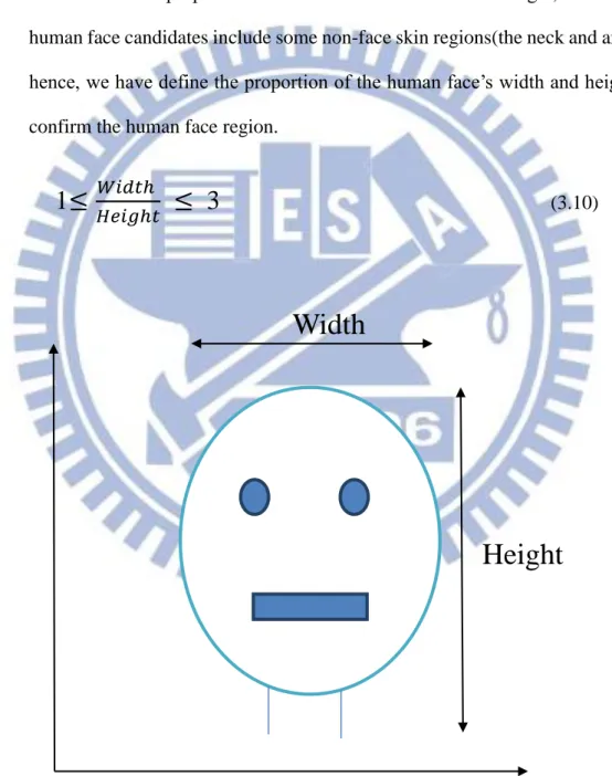
(II) The proportions of the human face’s width and height have to fit the (3.10). In

the general condition, human face’s height bigger than the width, the figure 3.1.4.1 show the proportion of the human face’s width and height, besides, the human face candidates include some non-face skin regions(the neck and arms) ,

hence, we have define the proportion of the human face’s width and height to confirm the human face region.

1≤

𝑊𝑖𝑑𝑡ℎ

𝐻𝑒𝑖𝑔ℎ𝑡

≤ 3

(3.10)

Figure 3.1.4.1 The proportion of the human face’s width and height.

Width

23

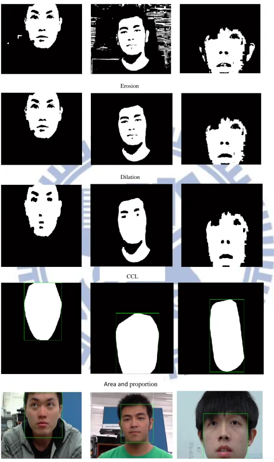
Before the detect eyes and mouth we have to human face detection, hence, I will

introduce the human face detection conclusion steps, which are as following figure

3.1.4.2 and the figure 3.1.4.3 shows Figure 3.1.4.2 flow chart per steps real human face

plots.

Figure 3.1.4.2 The flow chart of the human face detection. Skin color extraction

Area and proportion define

Erosion

CCL

Dilation

Binary image

24

Figure 3.1.4.3 To show real human faces detection of per step from the flow chart.

Skin color extraction and Binary image

Erosion

Dilation

CCL

Area and proportion define

25

3.1.4 Facial Feature Detection

In this thesis goal is to know human face faces where then get two information

which are orientation and angle, therefore, this thesis has to face detection and facial

feature detection. In the last sections already get human face position, which are known

the human face position where in per successive images. In this section wants to use

last section result then reach goal which are detection human facial feature, just like

eyes, mouth, nose and so on, but this thesis just to search two features on the human

face which are mouth and eyes. In this section will show more details how to detect

human eyes and mouth in this thesis.

3.1.4.1 Eye and mouth detection

The eye is the most significant and important feature in the human face, as

extraction of the eye are often easier as compared to other facial features. Eye detection

is also used in person identification by iris matching. Only those image region that

contain possible eye pairs will be fed into a subsequent face verification system.

Localization of eyes is also a necessary step for many face classification methods. Eyes

can be used for crucial face expression analysis for human computer interactions as

they often reflects a person’s emotions.

After last section of face detection, which are get human face ROI. In this step in

eye detection involves edge detection. Morphological techniques are used for boundary

detection. Dilation followed by erosion and the calculation of differences between the

two produces an image with boundaries. For the purposed at hand, this technique is

found to be more efficient that the laplacian edge detection. This is followed by suitable

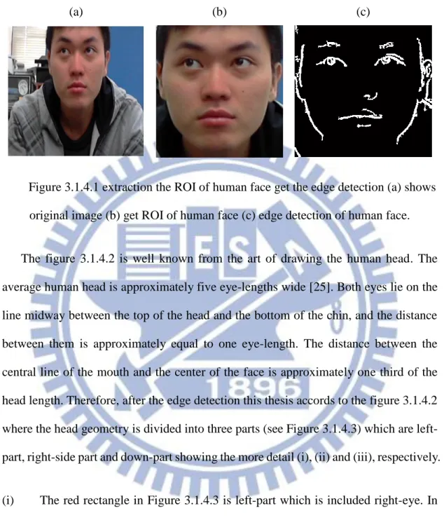
26

face and edge detection of human face.

(a) (b) (c)

Figure 3.1.4.1 extraction the ROI of human face get the edge detection (a) shows

original image (b) get ROI of human face (c) edge detection of human face.

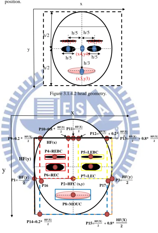
The figure 3.1.4.2 is well known from the art of drawing the human head. The

average human head is approximately five eye-lengths wide [25]. Both eyes lie on the

line midway between the top of the head and the bottom of the chin, and the distance

between them is approximately equal to one eye-length. The distance between the

central line of the mouth and the center of the face is approximately one third of the

head length. Therefore, after the edge detection this thesis accords to the figure 3.1.4.2

where the head geometry is divided into three parts (see Figure 3.1.4.3) which are

left-part, right-side part and down-part showing the more detail (i), (ii) and (iii), respectively.

(i) The red rectangle in Figure 3.1.4.3 is left-part which is included right-eye. In

the right-part we try to find the right-eye, therefore, in this part I label some

points and set some threshold to detect the right-eye position. P2 is human face centroid (RFC), P1 is the half human face (HF) of the coordinate y , P11 is half

human face of the coordinate x, P9 is half face of the coordinate x multiplied by

0.2, P10 is half face of the coordinate x multiplied by 0.8, P4 is right eyebrow

right-27

side part then set some threshold to search right-eye, the red rectangle is

connected to P9, P10, P1 and P2.there are two binary objects which are

right-eyebrow and right-eye in the red rectangle region, therefore, I have to determine

which one is the right-eye then mark it. Because the right-eyebrow centroid of

coordinate y is less than the right-eye centroid of the coordinate y, therefore, I

let P6 of the coordinate y bigger than P4 of the coordinate y. finally, I successful

detect right-eye.

(ii) The yellow rectangle in Figure 3.1.4.3 is left-part which is included left-eye. In

the left-part we try to find the left-eye, therefore, in this part I label some points

and set some threshold to detect the left-eye position. P2 is human face centroid (HFC), P3 is the half human face (HF) of the coordinate y, P11 is half human

face of the coordinate x, P12 is half face of the coordinate x multiplied by 0.2

and add half human face of the coordinate x, P13 is half face of the coordinate

x multiplied by 0.8 and add the half human face of the coordinate x, P5 is left

eyebrow centroid (LEC), P7 is left-eye centroid (LEC). After define all points

at left-side part then set some threshold to search left-eye, the yellow rectangle

is connected to P3, P7, P12 and P13.there are two binary objects which are

left-eyebrow and left-eye in the yellow rectangle region, therefore, I have to

determine which one is left-eye then mark it. Because the left-eyebrow centroid

of coordinate y is less than the left-eye centroid of the coordinate y, therefore, I

let P7 of the coordinate y bigger than P5 of the coordinate y. finally, I successful

detect left-eye.

(iii) The blue rectangle in Figure 3.1.4.3 is down-part which is included mouth. In

the down-part we try to find the mouth, therefore, in this part I label some points

and use the facial relation between eyes and mouth to check mouth position. P2

28

y, P3 is half human face of the coordinate y, P14 is half face of the coordinate x

multiplied by 0.2 and add half human face of the coordinate x, P15 is half face

of the coordinate x multiplied by 0.8 and add the half human face of the

coordinate x, P8 is mouth centroid (MOUC). After define all points at down part

then set some check conditions to search mouth, the yellow rectangle is

connected to P14, P15, P16 and P17. In the down-part have four relation

between eyes and mouth to check whether mouth is successful found position

or not. There are some mathematics function and mouth check which are

defined as below: The distance between right-eye and left-eye is assume Math1,

the distance between left-eye and mouth is assume Math 2, the distance between

left-eye and mouth is assume Math3, the distance between middle of eyes and

mouth is assume Math4.

Math 1:√(𝑥2 − 𝑥1)2_{+ (𝑦2 − 𝑦1)}2 _(3.11)

Math 2: √(𝑥1 − 𝑥3)2 _{+ (𝑦1 − 𝑦3)}2 _(3.12)

Math 3: √(𝑥2 − 𝑥3)2 _{+ (𝑦2 − 𝑦3)}2 _(3.13)

Math 4: √(𝑥4 − 𝑥3)2 _{+ (𝑦4 − 𝑦3)}2 _(3.14)

Check1: Check whether the mouth is in down-part or not.

Check2: 0.9 ≤ 𝑚𝑎𝑡ℎ1

𝑚𝑎𝑡ℎ4 ≤ 1.5 (3.15)

Check 3: Check whether the |math2-math3| < 0.25*math1 or not. (3.16)

Check4: Check whether the |math1-math4| < 0.25*math1 or not. (3.17)

29

position.

Figure 3.1.4.2 head geometry.

Figure 3.1.4.3 Head geometry divided to three part.

x

y

P2=HFC (x,y) 𝐇𝐅(𝐲) 𝟐 P1= 𝐇𝐅(𝐲) 𝟐 P3= P4=REBC _P5=LEBC P6=REC _P7=LEC P8=MOUC P11=𝐇𝐅(𝐗) 𝟐 P12=𝐇𝐅(𝐗) 𝟐 + 0.2* 𝐇𝐅(𝐗) 𝟐 P10=0.8 * 𝐇𝐅(𝐗)_𝟐 P13=𝐇𝐅(𝐗) 𝟐 + 0.8* 𝐇𝐅(𝐗) 𝟐 P9=0.2 * 𝐇𝐅(𝐗) 𝟐 P14=0.2* 𝐇𝐅(𝐗) 𝟐 P15=𝐇𝐅(𝐗)_𝟐 + 0.8* 𝐇𝐅(𝐗) 𝟐 HF(y) HF(x) x y h/5 h/5 h/3 h/2 h/2 P16 P17 h/5 h/5 (x1,y1) (x2,y2) (x3,y3) (x4,y4)

30

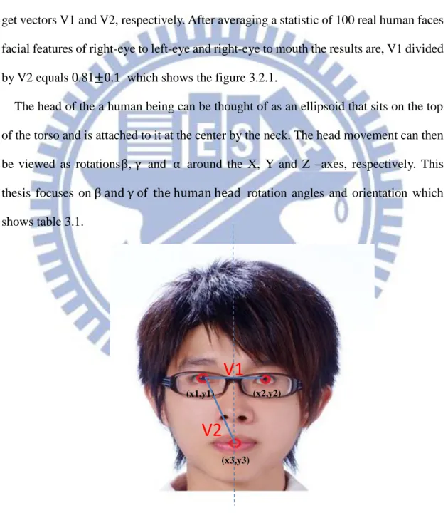
3.2 Geometric Facial Features

This thesis methods uses human’s eyes and mouth as feature, human’s eyes and

mouth have fixed proportion of face. Using this characteristic we can know the human’s

face orientation and rotation and angles. First, let the right-eye be the original point and

by the statistic average human’s right-eye to left-eye and right-eye to mouth, we can

get vectors V1 and V2, respectively. After averaging a statistic of 100 real human faces

facial features of right-eye to left-eye and right-eye to mouth the results are, V1 divided

by V2 equals 0.81±0.1 which shows the figure 3.2.1.

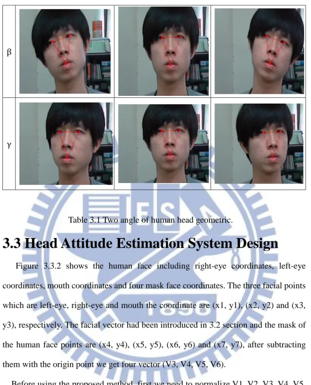
The head of the a human being can be thought of as an ellipsoid that sits on the top

of the torso and is attached to it at the center by the neck. The head movement can then

be viewed as rotationsβ, γ and α around the X, Y and Z –axes, respectively. This thesis focuses on β and γ of the human head rotation angles and orientation which shows table 3.1.

Figure 3.2.1 Geometric facial features.

(x1,y1) (x2,y2)

(x3,y3)

V1

V2

31

Table 3.1 Two angle of human head geometric.

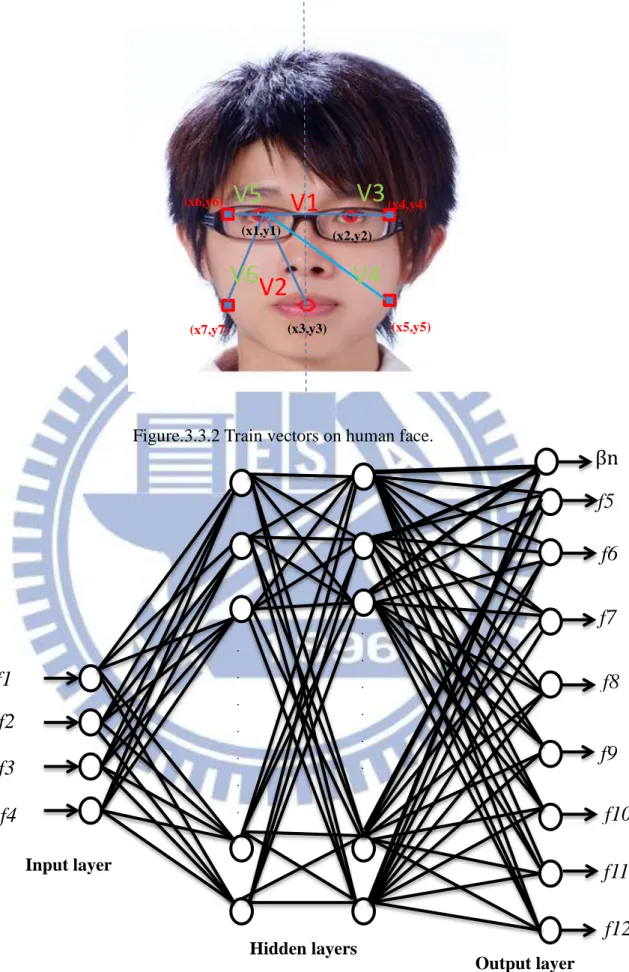
3.3 Head Attitude Estimation System Design

Figure 3.3.2 shows the human face including right-eye coordinates, left-eye

coordinates, mouth coordinates and four mask face coordinates. The three facial points

which are left-eye, right-eye and mouth the coordinate are (x1, y1), (x2, y2) and (x3,

y3), respectively. The facial vector had been introduced in 3.2 section and the mask of

the human face points are (x4, y4), (x5, y5), (x6, y6) and (x7, y7), after subtracting

them with the origin point we get four vector (V3, V4, V5, V6).

Before using the proposed method, first we need to normalize V1, V2, V3, V4, V5,

V6 and two angles of the human head geometry which are β and γ, the equations are from (3.18) to (3.30) : Dis = √(𝑣𝑥1)2+ (𝑣𝑦1)2 (3.18) f1 = Vx1/ Dis (3.19) f2 = Vy1/ Dis (3.20) f3 = Vx2/ Dis (3.21) β γ

32 f4 = Vy2/ Dis (3.22) f5 = Vx3/ Dis (3.23) f6 = Vy3/ Dis (3.24) f7 = Vx4/ Dis (3.25) f8 = Vy4/ Dis (3.26) f9 = Vx5/ Dis (3.27) f10 =Vy5/ Dis (3.28) f11= Vx6/ Dis (3.29) f12 =Vy6/ Dis (3.30)

where Dis is magnitude of V1.

Two angles of the human head geometry are limited between -30 and 30 degrees

because of the range of a normal human head geometry. Furthermore, before training

the angles have to be normalized, the angle degrees are shown in (3.31) and (3.32):

βn = β/30 (3.31) γn = γ/30 (3.32) where βn and γn are normalize range between 1 and -1.

The artificial neural network (ANN) is used to train the six normalize vectors and

normalize β angle, where two normalized vectors are the inputs which are right-eye to left-eye and right-eye to mouth, other normalized vectors are the outputs which are

four normalize vectors belong to extended normalize vectors of every four extend

points to subtract origin points . The normalized β angle and four extend normalized vectors are learned by the neural network structure in Figure3.3.3 based on the

back-propagation. The other normalized angle γ of human head geometric uses the same ANN structure to train four normalize vectors and normalize γ angle which shows in the Figure 3.3.4.

33

Figure.3.3.2 Train vectors on human face.

Figure 3.3.3 Neural network structure for β angle of the human head geometric.

(x1,y1) _(x2,y2) (x3,y3) (x5,y5) (x4,y4) (x6,y6) (x7,y7)

V1

V2

V3

V4

V6

Input layer Output layer Hidden layers

V5

. . . . . . . . . . . . . .

f1

f2

f3

f4

f5

f6

f7

f8

f9

f10

f11

f12

βn

34

Figure 3.3.4 Neural network structure for γ angle of the human head geometric.

For β angle of human head geometric neural network (βNN) based on the structure in Fig3.3.3, there include one input layer with four neurons, two hidden layer each layer

with 30 neurons, and one output layer with 9 neurons. The facial features vectors are

sent into 4 neurons of the input layer, represented by C (p), p =1, 2, 3, 4, correspondingly.

The p-th input neuron is connected to the q-th neuron, q=1, 2, 3, 4 ……. 30, of the first

hidden layer with weighting Wc1 (p, q). Besides, the q-th neuron of the first hidden layer

is also with an extra bias bc1 (q).Hence, there exists a weighting array Wc1 (p, q) of

dimension 4×30.The q-th of first hidden neuron is connected to the r-th neuron, r=1, 2, 3, 4…….30, of the second hidden layer with weighting Wc2 (q, r). There exists a weighting array Wc2 (q, r) of dimension 30×30. Besides, the r-th neuron of the second hidden layer is also with an extra bias bc2(r). Finally, the r-th neuron of the second

. . . . . . . . . . . . . .

f1

f2

f3

f4

f5

f6

f7

f8

f9

f10

f11

f12

γn Input layer Hidden layers Output layer

35

hidden layer is connected to the s-th neuron, s=1, 2, 3, 4…….9 with weighting array

Wc3 (r,s) of dimension 30×9, and a bias bc3 (s) is added to the output neuron.

Let the activation function of the hidden layer be the linear transfer function which

shows Fig.3.3.5 and the q-th output neuron Oc1 (q) is expressed as:

Oc1 (q) = purelin (n1 (q)), q =1, 2, 3, 4……….30. (3.33)

where

n1 (q) =∑4_𝑝=1𝑊𝑐1(𝑝, 𝑞)𝐶(𝑝) + 𝑏𝑐1(𝑞) (3.34)

Let the activation function of the second hidden layer be the linear transfer function

which shows Fig.3.3.3 and the second hidden neuron Oc2(r) is expressed as:

Oc2 (r) = purelin (n2(r)), r =1, 2, 3, 4……….30. (3.35)

where

n2(r) =∑20𝑞=1𝑊𝑐2(𝑞, 𝑟)𝑂𝑐1 (𝑞) + 𝑏𝑐2(𝑟) (3.36)

Let the activation function of the output layer be the linear transfer function which

shows Fig.3.3.3 and output neuron Oc3 (𝑠) is expressed as:

Oc3 (s) = purelin (n3 (s)), s =1, 2, 3……9. (3.37)

where

n3 =∑20_𝑟=1𝑊𝑐3(𝑟, 𝑠)𝑂𝑐2 (𝑟) + 𝑏𝑐3(𝑠) (3.38)

36

Figure.3.3.5 linear transfer function.

Figure.3.3.6 βNN.

For γ angle of human head geometric neural network (γNN) based on the structure in Figure3.3.4, there include one input layer with four neurons, two hidden layer each

layer with 25 neurons, and one output layer with 9 neurons. The facial features vectors

are sent into 4 neurons of the input layer, represented by G (p), p =1, 2, 3, 4,

correspondingly. The p-th input neuron is connected to the q-th neuron, q=1, 2, 3,

4 ……. 25, of the first hidden layer with weighting WG1 (p, q). Besides, the q-th neuron of the first hidden layer is also with an extra bias bG1 (q).Hence, there exists a weighting

array WG1 (p, q) of dimension 4×25.The q-th of first hidden neuron is connected to the

t-th neuron, t=1, 2, 3, 4…….25, of the second hidden layer with weighting WG2 (q, t).

There exists a weighting array WG2 (q, t) of dimension 25×25. Besides, the t-th neuron of the second hidden layer is also with an extra bias bG2(t). Finally, the t-th neuron of

the second hidden layer is connected to the u-th neuron, u=1, 2, 3, 4…….9 with

O

37

weighting array WG3 (t, u) of dimension 25×9, and a bias bG3 (u) is added to the output neuron.

Let the activation function of the hidden layer be the linear transfer function which

shows Fig.3.3.5 and the q-th output neuron OG1 (q) is expressed as:

OG1 (q) = purelin (n1 (q)), q =1, 2, 3, 4……….25. (3.39)

where

n1 (q) =∑4_𝑝=1𝑊𝐺1(𝑝, 𝑞)𝐺(𝑝) + 𝑏𝐺1(𝑞) (3.40)

Let the activation function of the second hidden layer be the linear transfer function

which shows Fig.3.3.5 and the second hidden neuron OG2 (t) is expressed as:

Oc2 (t) = purelin (n2(t)), t =1, 2, 3, 4……….25. (3.41)

where

n2(t) =∑20𝑞=1𝑊𝐺2(𝑞, 𝑡)𝑂𝐺1 (𝑞) + 𝑏𝐺2(𝑡) (3.42)

Let the activation function of the output layer be the linear transfer function which

shows Fig.3.3.5 and output neuron OG3 (𝑢) is expressed as:

Oc3 (u) = purelin (n3 (u)), u =1, 2, 3……9. (3.43)

where

n3 =∑20_𝑡=1𝑊𝑐3(𝑡, 𝑢)𝑂𝑐2 (𝑡) + 𝑏𝐺3(𝑢) (3.44)

The above operations are shown in Fig.3.3.7.

38

Chapter 4 Experiment Result

In the previous chapter, the three main steps of the proposed head attitude estimation

system are introduced. In this chapter, the experiment results of each step will be

expressed and the result of the proposed algorithm will be obtained by MATLAB

R2011b.

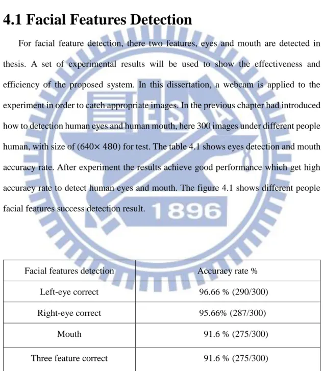
4.1 Facial Features Detection

For facial feature detection, there two features, eyes and mouth are detected in thesis. A set of experimental results will be used to show the effectiveness and

efficiency of the proposed system. In this dissertation, a webcam is applied to the

experiment in order to catch appropriate images. In the previous chapter had introduced

how to detection human eyes and human mouth, here 300 images under different people

human, with size of (640× 480) for test. The table 4.1 shows eyes detection and mouth accuracy rate. After experiment the results achieve good performance which get high

accuracy rate to detect human eyes and mouth. The figure 4.1 shows different people

facial features success detection result.

Facial features detection Accuracy rate %

Left-eye correct 96.66 % (290/300)

Right-eye correct 95.66% (287/300)

Mouth 91.6 % (275/300)

Three feature correct 91.6 % (275/300)

39

40

4.2 Geometric Facial Features

Thesis has to statistic more information of the geometric facial feature which are

β and γ . We don’t know human head rotation information, therefore, thesis manufactured a stereo facial model showing in the figure 4.2.1 which are showed the

appearance including a protractor and indicator which achieve more precise in the

statistic human attitude estimation system information. On the table, there are seven

points shows figure 4.2.2. Thesis uses red, green, blue colors represent right-eye,

left-eye, mouth and four points of mask human face.

41

Figure 4.2.2 RGB color label seven points.

After labeling red, green, blue colors automatic detected labeling, therefore,

thesis uses two steps to detect red, green and blue colors which shows figure 4.2.3, first,

gray level three colors and second step is binary three colors, finally, we can successful

automatic detect red, green, blue colors.

Figure 4.2.3 detection RGB colors.

P1 P2 P3 P6 P4 P5 P7 Left -eye right -eye mouth

Input image Gray R

Gray G Gray B Binary R Binary G Binary B Output image

42

4.3 Head Attitude Estimation System Design

This section shows the head attitude estimation system design experiment result,

including the neural network off-line training, test the neural network off-line training

performance and head attitude estimation final result.

4.3.1 Neural Network Off-line Training

This section focuses on the off-line training of the two neural networks, βNN and γNN, used in the head attitude estimation. It is known that different types of the head attitude estimation system requires different types of neural networks. Besides, all the

neural networks are designed to have three layers, the input layer, output layer and

hidden layer. The number of neurons of the input layer is chosen to the same as the

number of input data, so is the number of neurons of the output layer, corresponding to

the output data. However, how many neurons are needed for the hidden layer should be

determined by experiments, via neural network off-line training in this thesis.

According to the experiment, 𝛽NN performance are influenced to the distance between webcam and stereo facial model. The thesis divides two cases to determine

off-line training parameter.

Case1:

The 30CM distance from webcam to stereo facial model for case1. First, let’s find

the suitable number of neurons of βNN and γNN which will be applied to head attitude estimation system. The off-line training of the βNN is executed in difference cases, named as βNN-k, h where k is the number of neurons of the first hidden layer and is chosen from 10 to 30, where h is the number of the second hidden layer and is chosen

43

best while the pair of (k, h) are changed from (20, 20) to (30, 30), as show in Table

4.2.The performance from (20, 20) to (30, 30) are the same, thus, thesis choses (20, 20)

pair less neurons than (30, 30). Similarly, Table 4.3 shows the results of the off-line

training of the γNN. Obviously, the γNN-25, 25 is the best structure with minimal learning mean square error (MSE). Hence, the γNN-25, 25 will be used in the HAES.

Table 4.2 30CM distance of βNN off-line training parameter.

Experiments βNN-10,0 βNN- 20, 0 βNN- 30, 0 βNN- 10, 10 βNN- 20, 20 βNN- 25, 25 βNN- 30, 30 Learning Time(sec) 7.1 4.8 6.4 13.8 18.31 29.364 31.4 Epochs 321 163 259 273 383 600 658

First hidden neurons 10 20 30 10 20 25 30

Second hidden neurons 0 0 0 10 20 25 30 Tolerance 10−10 10−10 10−10 10−10 10−10 10−10 10−10 MSE (performance) 3.6× 10−4 3.83× 10−4 2.7× 10−4 5.6× 10−5 2.59× 10−5 2.67× 10−5 2.66× 10−5 Input neuron _{4 4 4 4 4 4 4} Output neuron 9 9 9 9 9 9 9

44

Table 4.3 γNN off-line training parameter

Case2:

It is all range of distance from webcam to stereo facial model for case1. First, let’s

find the suitable number of neurons of βNN which will be applied to head attitude detection system. The off-line training of the βNN is executed in difference cases, named as βNN-k, h where k is the number of neurons of the first hidden layer and is chosen from 10 to 40, where h is the number of the second hidden layer and is chosen

from 10 to 40. Based on the off-line training, it can be found that the performance is

best while the pair of (k, h) are changed from (30, 30) to (40, 40), as show in Table

4.4.The performance from (30, 30) to (40, 40) are the same, thus, thesis choses (30, 30)

pair less neurons than (40, 40).

Experiments γNN-10, 0 γNN-20, 0 γNN-30, 0 γNN-10, 10 γNN-20, 20 γNN-25, 25 γNN-30, 30 γNN-35, 35 Learning Time 17.24 12.3 19.75 20.48 28.14 31.9 33.8 36.7 Epochs 640 319 427 540 713 720 729 778 First hidden neurons 10 20 30 10 20 25 30 35 Second hidden neurons 0 0 0 10 20 25 30 35 Tolerance 10−10 10−10 10−10 10−10 10−10 10−10 10−10 10−10 MSE (performance) 3.7× 10−4 3.6× 10−4 3.6× 10−4 3.4× 10−4 4.61 × 10−5 4.6× 10−5 4.6× 10−5 4.61 × 10−5 Input neuron 4 4 4 4 4 4 4 4 Output neuron 9 9 9 9 9 9 9 9

45

Table 4.4 All distance range of βNN off-line training parameter.

4.3.2 Test neural Network Performance

In this section, this experiment will test the performance both of 𝛽NN and γNN. According to the experiment, the 𝛽NN performance is influenced by the distance between webcam and stereo facial model. The figure 4.3.1 shows the different distance

between webcam and stereo facial model image. There are two case in the βNN. The case1 is training data in 30 CM of the distance and case 2 is training data in all ranges.

The table 4.4 shows the training data in case1 of β NN accuracy rate relating two angle-scale and distance. In the table 4.5, obviously, the distance from 20CM to 30CM

had good performance, the distance from 35CM to 40CM is medium performance and

the distance from 45CM to 50CM had bad performance. The reason is the stereo facial

model closing the webcam and the pixels change a measure of the βNN information is very obvious. Otherwise, the stereo facial model is far away from the webcam and the

pixels change a measure of the βNN information extremely awful. The figure 4.3.2

Experiments γNN-10, 0 γNN-20, 0 γNN-30, 0 γNN-10, 10 γNN-20, 20 γNN-25, 25 γNN-30, 30 γNN-35, 35 γNN-40, 40 Learning Time 17.24 12.3 19.75 20.48 28.14 31.9 33.8 36.7 36.7 Epochs 640 319 427 540 713 720 729 778 778 First hidden neurons 10 20 30 10 20 25 30 35 35 Second hidden neurons 0 0 0 10 20 25 30 35 35 Tolerance 10−10 10−10 10−10 10−10 10−10 10−10 10−10 10−10 10−10 MSE (performance) 3.7× 10−4 3.6× 10−4 3.6× 10−4 3.4× 10−4 4.61 × 10−5 4.6× 10−5 2.57× 10−5 2.61× 10−5 2.58× 10−5 Input neuron 4 4 4 4 4 4 4 4 4 Output neuron 9 9 9 9 9 9 9 9 9

46

shows the histogram relates to accuracy rate and angle-scale of

orientation βNN in case1. In this plot, the accuracy rate accompanies the distance becoming extremely awful. In table 4.4, it is clearly observed that the angle-scale from

±0~ ± 20 had a good performance and the angle-scale ±21~ ± 30 was extremely awful. The reason is the angle-scale ±21~ ± 30 rotation was too extreme, hence the information of the βNN judge the accuracy angle. The figure 4.3.3 shows in the different angle-scale curves in case1, the βNN relating two accuracy rates and distance. Obviously, the curves shows the good performance when the angle-scale within ±0~ ± 20 and the curves shows the bad performance when the angle-scale within±21~ ± 30. The table 4.6 shows the training data including all distance range, the table shows

performance better than the training data only distance in 30CM. The figure 4.3.4 shows

histogram relates to accuracy rate and angle-scale of orientation βNN of the distance in all ranges. Figure 4.3.5 shows the different angle-scale curves in case2 .Table 4.7

shows γ NN accuracy rate relating two angle-scale and distance. Obviously, γNN performance are not influenced by the distance between webcam and stereo facial model. The reason is the pixels change a measure of the γNN information are very obvious in the per-independent angle-scale. The figure 4.3.6 shows histogram relating

two accuracy rate and angle-scale of orientation γNN. Obviously, the performance is very well in different distances. The figure 4.3.7 shows in the different angle-scale

curves, theγNN relating two accuracy rate and distance. In this plot, the accuracy rate is not influenced by the different angle- scale curves. Finally, the figure 4.3.8 shows the

HAES final result.

47

Figure 4.3.1The different distance between webcam and stereo facial model.

20CM 25CM 30CM 35CM 40CM 45CM 50CM 0°_~5° ₆°_~10° ₁₁°_~15° ₁₆°_~20° ₂₁°_~25° ₂₆°_~30° 20CM 100% 100% 96.5% 100% 100% 96.5% 25CM 96.5% 96.5% 95.5% 99% 95.5% 95.5% 30CM 97% 99% 100% 99% 93% 91.5% 35CM 95% 85.5% 97.5% 91% 71.5% 64% 40CM 96% 92% 92.5% 88.5% 64.5% 63% 45CM 79% 56.5% 51.5% 51% 29.5% 20% 50CM 76.5% 49.5% 48% 47.5% 19.5% 20% 0°_~−5° ₋₆°_~−10° ₋₁₁°_~−15° ₋₁₆°_{~ − 20}° ₋₂₁°_{~ − 25}° ₋₂₆°_{~ − 30}° 20CM 100% 100% 98.5% 100% 100% 97.5% 25CM 97.5% 98% 100% 100% 96% 91% 30CM 100% 100% 99% 100% 92.5% 91% 35CM 96.5% 86.5% 95.5% 89.5% 73.5% 68.5% 40CM 97.5% 90.5% 89.5% 91.5% 60.5% 61.5% Distance Accuracy rate Distance Accuracy rate