國 立 交 通 大 學
電子工程學系 電子研究所碩士班
碩
士
論
文
基於格狀特徵值之推舉式人臉分類器
Boosting-kind Face Classifier Based on
Grid Features
研 究 生:駱俊晟
指導教授:王聖智 博士
基於格狀特徵值之推舉式人臉分類器
Boosting-kind Face Classifier Based on Grid Features
研 究 生:駱俊晟 Student:Lo Chun Chen
指導教授:王聖智博士 Advisor:Dr. Sheng-Jyh Wang
國 立 交 通 大 學
電子工程學系 電子研究所碩士班
碩 士 論 文
A Thesis
Submitted to Department of Electronics Engineering & Institute of Electronics College of Electrical and Computer Engineering
National Chiao Tung University in partial Fulfillment of the Requirements
for the Degree of Master in
Electronics Engineering September 2008
Hsinchu, Taiwan, Republic of China
基於格狀特徵值之推舉式人臉分類器
研究生:駱俊晟 指導教授:王聖智 博士
國立交通大學
電子工程學系 電子研究所碩士班
摘要
偵測是人眼視覺中的一項重要功能,但對於電腦視覺仍是一大挑
戰。在本論文中,我們提出一種用於推舉式人臉偵測器的新的特徵:
「格狀特徵」,它有三項特點:一、特徵以格子網狀的形式來表現,
藉此減少特徵的數量與特徵之間的重疊性。二、以漸進的方式擴大特
徵空間,將簡單的特徵結合成一更具分辨能力的新特徵。三、加入「變
化量」做為測量方法,用來獲取使用「總合」測量所不能獲取的資訊。
實驗中,我們訓練了一個由五級分類器串接而成的人臉分類器,總共
使用了兩百個弱分類器(特徵+閾),前面四級分類器我們使用對稱
的特徵使得偵測更為穩定強健。在兩組測試圖檔中,使用格狀特徵的
分辨能力比傳統 Harr 特徵效果來得更好。
Boosting-kind Face Classifier Based on
Grid Features
Student: Lo Chun Chen Advisor: Dr. Sheng-Jyh Wang
Department of Electronics Engineering, Institute of Electronics
National Chiao Tung University
Abstract
Detection is an important function of human vision. However, it is
still a big challenge for computer vision. In this thesis, we propose a new
grid feature for boosting-kind face classifiers. The grid features contain
three major properties: (1). they use a grid representation to reduce the
number and redundancy of features; (2). they adopt a progressive way to
combine simple features together to form more complex and
discriminative features; and (3). they add the variance measure to
discover more information than the sum measurement. We train a face
classifier cascaded by 5 layers and use 200 weak learners in total. In the
first four layers, we only use symmetric features for the sake of
robustness. Based on the experiments over two test patterns, our grid
feature performs better than the commonly used traditional Harr-like
feature.
誌謝
我要感謝 王聖智老師這兩年的指導;老師給予充分的空間讓我
探索尋找喜歡的研究方向,每次討論中以身作則地告訴我做研究應該
有的態度與責任,從老師身上我學習到身為讀書人該有的做為。另外
我也要感謝 黃日鋒副組長與工研院 W200 同仁,除了給予我學術上
的指導也帶給我家庭般的溫暖。
在這兩年中還有很多要感謝的人事物,例如下班後特地撥出時間
和我討論的信嘉學長,經常提醒幫助我的亦安,以及在日本認識的許
多朋友…。要感謝的人太多了,除了謝天,我也希望今後能有一番作
為,不辜負你們的厚愛。
Content
Chapter 1. Introduction ... 1
Chapter 2. Backgrounds... 2
2.1 Feature... 2
2.1.1 Harr- like feature ... 2
2.1.2 Part-based feature... 5
2.2 Boosting ... 6
2.2.1 PAC Learning ... 7
2.2.2 Adaboost... 8
Chapter 3. Proposed Method ... 12
3.1 Grid Representation ... 12
3.2 Progressive Feature Space ... 15
3.3 Variance Measurement ... 22
Chapter 4. Experiments ... 25
4.1 Training Data ... 25
4.1.1 Positive training data... 25
4.1.2 Negative Data... 26
4.2 Symmetric Property of Front Face... 29
4.3 Cascade Structure and Bootstrap Method ... 31
4.4 Results ... 33
4.4.1 Comparison Between Grid Feature and Harr- like Features on Test Pattern O ne... 33
4.4.2 Comparison Between Grid Feature and Harr- like Features on Test Pattern Two ... 37
4.4.3 Summery of Experiments ... 40
Chapter 5. Conclusion ... 41
List of Figures
Figure 2-1(a) 3 kind Harr-like features (2, 3 and 4 rectangles) (b) The first 2 selected
features ... 2
Figure 2-2 Samples of Harr-like features... 3
Figure 2-3 Harr-like features are like highly dependent vector set ... 4
Figure 2-4 The threshold for Harr-like features... 4
Figure 2-5 Integral images... 5
Figure 2-6 Five steps to construct part-based features... 6
Figure 2-7 Overfitting ... 8
Figure 2-8 Training data are linear separated in the weak learner space ... 10
Figure 3-1 Two similar Harr-like features ... 12
Figure 3-2 The hypothesis space of boosting-kind classifiers... 13
Figure 3-3 The grid representation reduces many redundancies in Harr-like features ... 13
Figure 3-4 grid-Harr-like features ... 14
Figure 3-5 The error rates of two classifiers with Harr-like features and grid-Harr-like features ... 14
Figure 3-6 The 6*6 grid structure ... 15
Figure 3-7 Combine two simple features to a more discriminative feature ... 16
Figure 3-8 Features at iteration 1 in progressive feature space process ... 17
Figure 3-9 Features at iteration 2 in progressive feature space process ... 17
Figure 3-10 Features at iteration 2 in progressive feature space process ... 18
Figure 3-11 the relation between the progressive feature space and the hypothesis space ... 18
Figure 3-12 constructed features in the progressive process ... 20
Figure 3-13 Performances of two classifiers (with Harr-like features and with our features) ... 21
Figure 3-14 Performances of 10*10 and 6*6 grid sizes ... 22
Figure 3-15 (a) The sum of two rectangles are close. (b) The rectangles with new measurement may be a good feature ... 23
Figure 3-16 the grid feature with the variance measurement ... 23
Figure 3-17 Performances of three classifiers (Harr-like features, grid features with sum measurement and grid features with sum & variance measurement). ... 24
Figure 3-18 The first three features with the variance measurement... 24
Figure 4-1 Positive training data (a) only face (b) include the hair ... 26
Figure 4-3 Choose the negative data as close to positive data as possible ... 27
Figure 4-4 The procedure to find our negative set ... 28
Figure 4-5 (a) negative set A (b) negative set B (c) negative set C ... 29
Figure 4-6 Train features on half side then map them to the other side of face... 30
Figure 4-7 Error rates to different thresholds ... 30
Figure 4-8 The cascade structure with the bootstrap method ... 32
Figure 4-9 First two features of each stage... 34
Figure 4-10 ROC curves of two classifiers (with grid features and Harr-like features) ... 35
Figure 4-11 Some detected photos by the classifier with grid features ... 36
Figure 4-12 ROC curves of two classifiers (with grid features and Harr-like features) on CMU test pattern ... 37
Figure 4-13 Some detected photos in CMU test file by the classifier with grid features ... 39
List of Tables
Table 4-1 The detection rate to false positive rate of the classifier with Harr-like
features ... 35
Table 4-2 The detection rate to false positive rate of the classifier with grid features 35 Table 4-3 The detection rate to false positive rate of the classifier with Harr-like
features ... 38
Chapter 1.
I
NTRODUCTION
Detection is a basic and important function of human vision; even a young child can easily do it. However, it’s still a big problem for computer vision. We face the following challenges: 1. View point variation. 2. Illumination change. 3. Occlusion. 4. Different scales. 5. Deformation. 6. Background Clutter. [6] Until today, we are not clear how the human vision overcomes these difficulties.
Above all things, the face is one of the most interesting objects we want to detect. In many applications, if we achieve the face detection, we could do following processes, for example, tracking, identification and face expression extraction.
In the computer vision, we usually use statistic approaches to deal with the detecting issue. We formulate it as a classification problem. There are two main different ways to solve it; one is the generative method and the other is the discriminative method. The former tries to model the prior distribution of faces and other classes. The later just considers the posterior probability to find a boundary. In this paper, we adopt the boosting-kind classifier which belongs to the discriminative method. One reason is because we believe that the distribution of face isn’t easy to be approximated by simple model.
In chapter 2, we introduce the background of using boosting-kind classifiers on the face detection. We focus on how to select features and how does the boosting method work. In chapter 3, we propose a new kind feature, grid feature, to extract more information from human faces. We also discuss the relation of features and the classifier’s hypothesis space here. In chapter 4, we describe the detail of training a boosting-kind classifier with our grid features. And we show the performance comparisons between grid features and Harr- like features. We have our conclusion in chapter 5.
Chapter 2.
B
ACKGROUNDS
2.1
F
EATURE
How to design and select features is an important issue in the classification and machine learning. It transfers raw data from the original space into a new space which Euclidean distance is more suitable to measure our data. Here we introduce two ways to create suit-able features for the face detection.
2.1.1
H
ARR
-
LIKE FEATURE
In 2001, Viola and Jones used Harr- like features with Adaboost classifiers to construct a fast real-time face detection system [4]. They chose it because of the advantage of boosting- kind classifiers and the fast computation character of Harr-like features. In their system, they uses three kind Harr- like features (using 2, 3 and 4 rectangles) as in Figure 2-1(a) and the first two selected features by Adaboost are showed in Figure 2-1(b)
Figure 2-1(a) 3 k ind Harr-lik e features (2, 3 and 4 rectangles) (b) The first 2 selected features
How do we compute Harr- like features? First, we sum up every pixel in each rectangle of the feature. Then we use the sum of white rectangles to minus the sum of black rectangles. Every feature will produce a real number in this way. App lying these features on training data or test images, we can transfer inputs from the original space
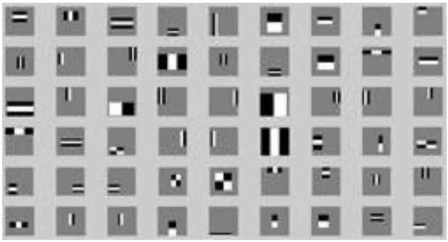
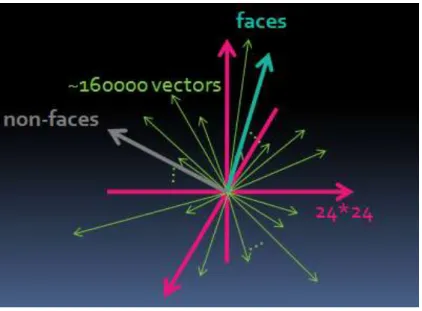
to the feature space. Viola and Jones used the above three kind Harr- like features to create ~160’000 Harr-like features in 24*24 windows as their feature space . We show some samples in Figure 2-2
Figure 2-2 Samples of Harr-lik e features
Why do we need a so large feature space? The reason is we want to find the best feature from the set to construct our weak learner. We need to create enough candidates for selection; otherwise the best one might be still useless. The “best” here means the feature can distinguee weighted training faces (positive data) from weighted training non-faces (negative data) better than the others. We can look these Harr- like features as a highly dependent vector set. We project training faces and non- faces to those vectors. In ~160’000 vectors, we pick out the one which separates two projected data mostly. We record the separating threshold and call the feature plus the threshold as a weak learner (a weak classifier). We use Figure 2-3 and Figure 2-4 to illustrate the idea.
Figure 2-3 Harr-lik e features are like highly dependent vector set
In the origina l pixe l space, the ~160’000 Ha rr-like features are like h ighly dependent vector set. We project train ing faces and non-faces on these vectors.
Figure 2-4 The threshold for Harr-lik e features
After we pro ject tra ining data to those vectors, we find a threshold for every feature. We pic k out the best one which separates projected data mostly. The feature plus the threshold is called the wea k learner.
In order to accelerate the detection time, Viola used integral image to compute these features. We use Figure 2-5 to explain it. When we input an image, we use top left corner P and every pixel Xi to form different size rectangles. Then we sum up all pixels in the rectangle and record it at the bottom right corner Xi. After we’ve done this, we can compute Harr-like features very fast. For example, when we want to compute the feature in the right side of Figure 2-5, we only use the value of X4 minus 2 times the value of X2. The computation is only about 5~10% comparing to original one (it depends on the Harr- like feature size).
Figure 2-5 Integral images
2.1.2
P
ART
-
BASED FEATURE
In 2007, Torralba and et al invented a system sharing visual features for multi-class and multi- view object detections. [7] In his system, he also used a boosting-kind classifier but with different features. He chose part-based features inspired from Vidal-Naquet’s work. We use following 5 steps and Figure 2-6 to introduce the feature.
Five steps to construct part-based features:
1. Collect training images and mark the object we want to detect. Resize images to make marking area in 32*32 windows.
2. Extract patches from the object windows as templates and record the location. The template sizes are from 4*4 to 14*14 pixels. One template plus the location is equal to a feature.
3. Compute the normalized correlation between images and patch Pi
4. Compute the convolution of step3 output and the relative patch location mask.
5. Use the center value of the object windows as the positive training data ’s output of this feature. Samples outside the windows are outputs of negative data.
Figure 2-6 Five steps to construct part-based features
In step 1 and 2, usually we collect about 2000 patches as our templates. These patches are parts of the object we want to detect. After we run boosting algorithm to combine some good ones of all patches together, we can look them as voters. If a test image can pass the classifier, it means that many parts of this image are similar to the object. That’s why we call them part-based features. In step 3 and 4, Torralba used the convolution of relative location instead of the full object template because it allows some flexibility.
2.2
B
OOSTING
Boosting is a method to combine many simple “hypotheses” together to form a more accurate and complex hypothesis. We can use it to combine weak learners (weak classifiers) together to form a stronger classifier. It is based on PAC learning and has many good characters, such like “robust”, “not easy overfitting”, “fast convergence”... After Freund and Schapire proposed the first practical boosting algorithm, Adaboost,
many other kinds boosting algorithm are invented in recent years [1][2][3]. In 2001, Viola used Adaboost classifier on face detection and achieved a remarkable result. After that, the boosting method is the state of art o n the fast face detection issue. Here we introduce PAC learning first. Then we discuss the detail of Adaboost algorithm. Finally, we prove the upper bound of the error.
2.2.1
PAC
L
EARNING
Learning methods are more and more popular in recent years. One of t he reasons we use them is because we don’t know the real model and distribution. Instead of using the simple model to approximate it, we collect many training data and try to find some regulations. In the training process, we learn to find a hypothesis h with low error rate on training data (errˆ ( )D h ) then use it to bound the expected error
(errD( )h ). In other words, we want to discover some rules from training data and hope
these rules executable for future inputs. However, there is always a chance that it is impossible to arbitrarily bound the error of expected error (err hD( )) because of a highly abnormal training set. Thus, we want the algorithm generating h to be
“probably approximately correct” (PAC). The math form is in Eq.2-1 [11].
ˆ
Pr[err hD( )err hD( ) ] 1 Eq.2-1 There is a nice theorem named “uniform convergence” connecting the training error and the expected error.
By uniform convergence theorem, we can derive the bound of expected error.
ln 2 ln(1 / ) ˆ ( ) ( ) 2 D D H err h err h m Eq. 2-2
Uniform convergence theore m
Given m examples, assume H is finite, with probability 1
h err hD( )err hˆD( ) if 2 1 ln ln ( ) H m O ,
For a fixed , we can see that there are 3 factors to alter the upper bound. The first factor is the training error; when we minimize it, the upper bound of expected error is also minimized. The second factor is the size of the hypothesis space; the larger size of the hypothesis space leads to larger upper bound. The last factor is the number of training data. It is inverse to the bound, and that’s why we usually use large training data. These factors are not independent, especially the front two factors. When we enlarge the size of the hypothesis space, usually we can get better training error. However, the smaller training error doesn’t ensure better expected error because we also increase the second term of the upper bound. This phenomenon is called “overfitting”. We use the following Figure 2-7 to express it.
Figure 2-7 Overfitting
2.2.2
A
DABOOST
Working in Valiant’s PAC learning model, Kearns and Valiant posed the question of whether a “weak” learning algorithm can be boosted into a stronger learning algorithm. The answer is yes. In 1995, Freund and Schapire came up with the first practical boosting algorithm, Adaboost. It combines “weak” learners h which have error rate just better than random guess into a strong classifier.
1 T t t t
f
h
Eq. 2-3.
The main idea of Adaboost is to focus on miss-classified training data. At each time, Adaboost picks the best weak learner which generates the smallest weighted error (t 1/2t ). Then it increases the weight of miss-classified data and
decreases the weight of right ones. In next round, it finds a new weak learner minimizing reweighted error. After T rounds, the strong classifier can achieve a much smaller error ( ( ) 2 t(1 t)
t
error f
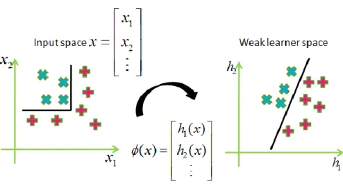
). The overall algorithm is as following:The final hypothesis is the linear combination of weak learners. It means that after we transfer positive and negative training data into the weak learner space, we can linear separate them. We use Figure 2-8 to illustrate this idea.
Adaboost algorithm
Input: N examples{( ,x y1 1)( ,x y2 2),..., (xN,yN)}, y is the class label of i x i
Initialize: d1n 1 N
for all n = 1, 2… N For t = 1…T
1. Find the best weak learner h xt: { 1} to minimize weighted
error 1
(
(
))
N t
t n
d I y
n nh x
t n
2. Compute hypothesis weight
1
log(
1
)
1
log(
1
)
2
2
1
t t t t t
3. Update example distribution
d
nt 1d
ntexp(
ty h x
n t( )) /
nZ
t
, 1exp(
(
))
N t t t n t n n nZ
d
y h x
EndOutput: final hypothesis
1
( )
T final t t tf
h x
1 ( ) ( )
exp(
(
))
exp(
)
exp(
)
(1
) exp(
)
exp(
)
t t n n n n N t t t n t n n n t t n t n t y h x y h x t t t tZ
d
y h x
d
d
*1
1
((1
) exp(
)
exp(
))
0
log(
)
2
t t t t t t t td
d
Figure 2-8 Training data are linear separated in the weak learner space
In the algorithm, tis the coefficient to combine weak learners. How do we choose the tin Adaboost algorithm? We look Z as a lose function and try to find t
a suitable tto minimize it.
The last thing we want to prove is the upper bound of the error. We want to show a few weak learners can theoretically generate a stronger classifier.
The upper bound of the error
Step 1: unwrapping recurrence:
1 1 1
1
(exp(
( )) /
)
(exp(
( )) /
)
exp(
( ))
1
final T n n n T n n T n n t td
y h x
Z
y h x
Z
m
y f x
m
Z
Step 2: training error t t
Z
Train error1
1
0
nm
if
y f x
n(
n)
0
else
1
exp(
n(
n))
t n ty f x
Z
m
Step 3:Z
t
2
t(1
t)
( ) ( )exp(
)
exp(
)
(1
) exp(
)
exp(
)
t n n t n n t t n t y h x t n t t t t t y h x
Z
d
d
Set1
1
ln(
)
2
t t t
Z
t
2
t(1
t)
Then we can get that
( )
2
t(1
t)
tChapter 3.
P
ROPOSED
M
ETHOD
Our work focuses on proposing a new feature named “grid feature” for the boosting-kind face classifiers. There are three main differences comparing to before works. First, we adopt the grid representation to construct our features so we can decrease the feature space size. Second, unlike Viola and Jones limited their feature in 3 kinds Harr- like features, we use a progressive method to gradually enlarge our feature space toward “good” direction. Finally, we add the variance measurement to discover more information than the sum measurement used in Harr- like features. We introduce the detail in following sections.
3.1
G
RID
R
EPRESENTATION
Viola and Jones used 3 kind Harr- like features to create nearly 160’000 Harr-like features as their feature space for picking weak learners. There are many fea tures very similar in this set. For example, Figure 3-1 shows two Harr- like features; they are just a little different in their position and size. The highly dependent and redundant properties of those Harr- like features cause the difficulty of training. If we don’t only use 3 kind Harr- like features but want to add more varieties to the feature space. It might increase the features to hundreds of millions. It’s impossible to train a classifier with such a huge feature space.
Figure 3-1 Two similar Harr-lik e features
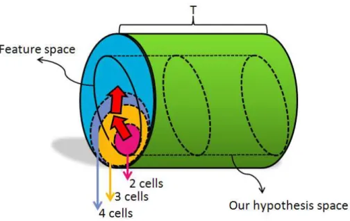
Besides the training problem, a huge feature space also has risk to make overfitting. From Eq.2-2, we showed that the complexity of hypothesis space influences the upper bound of the test error. The hypothesis space of the boosting-kind
classifier is controlled by two factors. O ne is the number of weak learners and the other one is the feature space for picking weak learners (because the threshold is fixed after we pick the feature). When we enlarge the feature space, we also increase the complexity of hypothesis space. As a result, even if we have the ability to train a classifier with hundreds of millions features, it still not a good idea because of the overfitting risk. We use Figure 3-2 to illustrate the relation between the feature space and the hypothesis space.
Figure 3-2 The hypothesis space of boosting-k ind classifiers
Considering above two problems, we decide to construct our features based on the grid representation. O ur idea is inspired from Li Fei Fei’s tutorial course in CVPR 2007. She showed that the grid representation has good performance on the category classification. In other words, when we use the grid representation, we still have enough information to classify the image.
If we apply the grid representation on original Harr- like features, we can reduce the redundancy. For example, in Figure 3-3, we can use the right side feature to approximate features on the left side.
Figure 3-3 The grid representation reduces many redundancies in Harr-lik e features
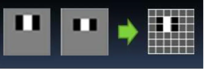
In order to verify the influence of the grid representation, we train two classifiers with different features. O ne classifier uses original Harr- like features and the other one uses “grid-Harr- like features”. The grid-Harr- like feature means we round off the rectangles to the near grid. Now the rectangles of Harr- like features can’t be placed at arbitrary places and the sizes are also limited. We can see the cell of grid as a unit and each Harr- like feature is composed of integral cells. We use Figure 3-4 to illustrate this idea.
Figure 3-4 grid-Harr-lik e features
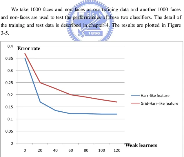
We take 1000 faces and non- faces as our training data and another 1000 faces and non- faces are used to test the performances of these two classifiers. The detail of the training and test data is described in chapter 4. The results are plotted in Figure 3-5.
Figure 3-5 The error rates of two classifiers with Harr -lik e features and grid-Harr-lik e features
0 0.05 0.1 0.15 0.2 0.25 0.3 0.35 0.4 0 20 40 60 80 100 120 Harr-like feature Grid-Harr-like feature Weak learners Error rate
There is a gap between the error rates of two classifiers but the one with grid-Harr- like features is still notable of its classification ability.
In summary, the grid representation can reduce space redundancies and is not easy to overfitting. In next two sections, we will show how to construct our features based on the grid representation to compensate the gap and even achieve better performance.
3.2
P
ROGRESSIVE
F
EATURE
S
PACE
In the above section, we used Harr-like features to discuss the influence of the grid representation. We compared original Harr- like features to grid-Harr- like features. Now we want to ask that if we don’t use Harr- like features, how we create features based on the grid form. Considering the 6*6 grid structure (see Figure 3-6, we sum up every pixel inside of each cell. Then we can use {-1,0,+1} coefficient set to arbitrarily combine any cells of the grid to form a new feature. In other words, we have
36 2 36 3 36 36 36
1 2 3 36
2C +2 C 2 C ...2 C possible combinations (it only considers {-1,0,+1} combination coefficients).
Figure 3-6 The 6*6 grid structure
In each feature, we use the sum of every pixe l in b lack ce lls to minus the sum in wh ite cells.
It’s hard to search all possible combinations so we need to have a strategy to find the suitable combination of cells as our feature. This problem is very similar to the classification problem. We want to find a boundary to separate two classes but there are too many choices. If our classifier is simple, it can’t distinguish them very well. If the classifier is very complex, it has the risk to overfitting. When we face this problem, we use boosting to combine weak classifiers together to form a stronger classifier. Using boosting method, we can overcome the dilemma above. This idea inspires us for finding the combination of cells in the same way.
Since it’s hard to directly find the combination of cells to form our features, we start from simple features which contain only few cell combinations. We build a simple feature set and pick out several good ones. “Good” means it has discrimination for training faces and non- faces. Then we combine some of these features to form a more complicated feature. We use Figure 3-7 to demonstrate our idea.
Figure 3-7 Combine two simple features to a more discriminative feature
There is a drawback in above idea. We can’t ensure all more complicated features perform better than simple ones. So we need to preserve those simple features in case of that situation. In other words, every time we keep original feature space and use the picked features to create more features. Add these new features to original space to form a new feature space. We can not only do this process one time to gradually enlarge our feature space. Using this method, we don’t construct a huge feature space at first time (for example, Viola and Jones used ~160’000 features). O ur feature space size is determined by how many iterations we run. We use the following figures to illustrate it.
Figure 3-8 Features at iteration 1 in progressive feature space process
At first iteration, we use only one cell to construct our feature set. There are total 36 features. (We don’t consider the minus sum of each cell because they have the same discriminative ab ilities)
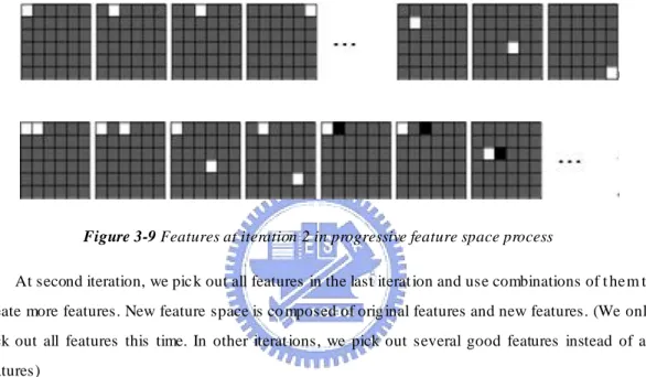
Figure 3-9 Features at iteration 2 in progressive feature space process
At second iteration, we pic k out all features in the last iterat ion and use combinations of t he m to create more features. New feature space is co mposed of orig inal features and new features. (We only pick out all features this time. In other iterat ions, we pick out several good features instead of all features)
Figure 3-10 Features at iteration 2 in progressive feature space process
At third iteration, we p ick out M good features (the number we need to choose by hands) fro m the last iteration. We use all possible comb inations of these picked features and original 36 features to create new features. This process keeps going until T iterations finish. Yellow means multip ly by 2.
Each time we pick good features to increase our feature space. That ’s why we call the space progressing toward good direction. We show the relation between the progressive feature space and the hypothesis space of boosting-kind classifiers in Figure 3-11.
Figure 3-11 The relation between the progressive feature space and the hypothesis space
In the above process, we start from all possible combinations of features with one cell but it’s not necessary. One can start with more cells. For example, if we start with 2 cells, we have C +2 C =2556136 362 features at first iteration. And in the next iteration, we will have 2556+2 C 25562 features. It cost more training time. We state this progressive process in math form in next page.
Progressive Feature Space Training set:
X
{ ,... }
x
1x
n
,x
i
m
Grid measurement transfer matrix:
G
r m , r = # grid
2 measurements 1.y
i0
Gx
i
,
Y
r n0
{ ,... }
y
10y
n0
2. Initial coefficient matrix:
1 0 0 0 0 0 k r k
c
C
c
,c
i: set arbitrary 2 elements = 1 or -1,others = 0,
k
0
2
C
2r 3. For t = 1,2,…,T (1) 1 1{ ,...,
|
}
t t t t t t t n i i k nZ
z
z
z
C y
, 1 tk
is the dimension of currentz
i
(2) Use Boosting algorithm to find the best #
r
t features with thresholds(3) 1 ( ) t t t t t r n r r
Y
Y
Z
(4) 1 ( ) t t t t t k r r t kc
C
c
c
i: set arbitrary 2 elements = 1 or -1,others = 0,
2
2 t t r rk
C
(5)r
r
r
t EndFirst, we transfer pictures from the raw data space ({ ... }xi xn ) to the grid
measurement space{ ... ... }y10 yi0 yn0 . We can see each grid measurement as a feature. At iteration t = 1, we use {-1, +1} to combine any two of y as a new feature to form i0
the first hypothesis space. Then we apply boosting algorithm on the space to pick out “good” few features (so we say that it’s toward the good direction). Adding these features and original features (each grid measurements) together, we get y . At 1i
iteration t =2, we combine any 2 features of y as a new feature to form the second i1
hypothesis space and keep on. t t 1
i i
y y numbers of features we picked at iteration t. When t increases, we gradually enlarge the hypothesis space and find more complicated features.
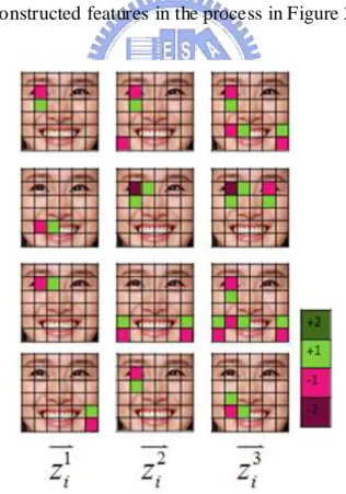
We give some constructed features in the process in Figure 3-12.
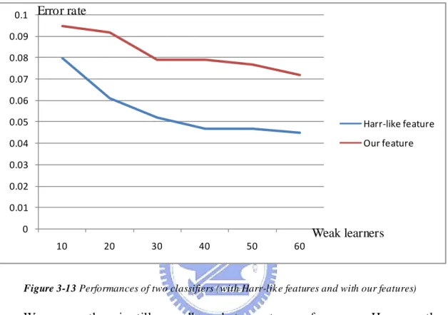
Now we want to compare the features we found to original Harr- like features. We use 1000 training faces and 1000 training non-faces to train two classifiers. O ne uses our features and the other one use Harr-like features. The grid size we chose is 6 cells*6 cells and we run 3 iterations in the progressive process. The test data are 1000 faces and 2000 non- faces. The result is in Figure 3-13.
Figure 3-13 Performances of two classifiers (with Harr-lik e features and with our features)
We can see there is still a small gap between two performances. However, the gap is less than 3%. We can run more iteration to get even closer results. And in next section, we will add another measurement to our features. It can cross the gap to achieve better performance.
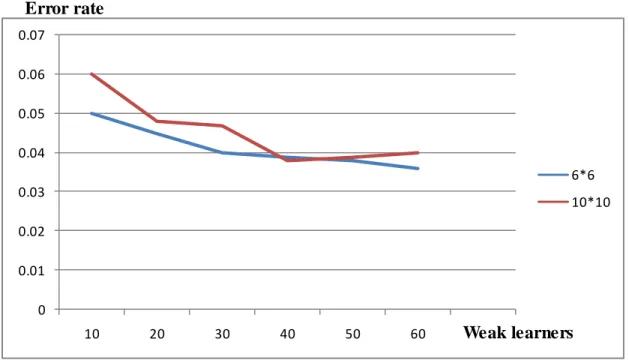
The last issue we want to discuss in this section is the grid size. Different grid sizes have different performances and training times. In our experiments, we’ve tried 10 cells *10 cells, 6 cells*6 cells and 5cells *5cells three sizes in 30*30 windows. They all use the same progressive strategy to create features. Again, the training data are 1000 faces and 1000 non-faces and the test data are 1000 faces and 2000 non- faces. The performances of former two are very close and much better than the later one. We only plot the performances of former two here.
0 0.01 0.02 0.03 0.04 0.05 0.06 0.07 0.08 0.09 0.1 10 20 30 40 50 60 Harr-like feature Our feature Error rate Weak learners
Figure 3-14 Performances of 10*10 and 6*6 grid sizes
Although their results are very close, we notice there is a little overfitting in 10*10 grid size case. So in later experiments, we always use 6*6 grid size. This also supports our words that the grid representation is less chance to have overfitting (as long as we use too big grid size or too small cell size).
3.3
V
ARIANCE
M
EASUREMENT
In the above sections, we always use the sum measurement in each cell of the grid. The goodness is that the computation is very easy and fast. The drawback is that sometimes the sum measurement can’t give us enough information. Or we can say the sum measurement has no discrimination in some situations. For example, in Figure 3-15 (a) the sums of two rectangles are very near. It can’t distinguish the mouse with many details from the smooth cheek. In Figure 3-15 (b), if we can apply a measurement which tells the difference between two green rectangles, we can use them to construct a good feature.
0 0.01 0.02 0.03 0.04 0.05 0.06 0.07 10 20 30 40 50 60 6*6 10*10 Weak learners Error rate
Figure 3-15 (a) The su m of two rectangles are close. (b) The rectangles with new measurement may be a good feature
Because of the above defect, we bring in another measurement, variance. We not only compute the sum of each cell but also compute the variance. There are two main advantages to use the variance as our measurement. First, it’s the second moment which tells us extra information than the first mo ment. Besides, the computation is affordable. After we compute the sum of each cell, we already know the means and it lessens the computation of variance. We use Figure 3-16 to illustrate what the feature looks like after we add the variance measurement.
Figure 3-16 the grid feature with the variance measurement
The right side is a grid feature. It equivalent to
( )
( )
( )
( )
sum J
sum I
variance L
variance J
Eq 3-1 We want to know the influence of the variance measurement so we train two classifiers again. This time we use the same training data and test data in order to compare with the results in the before experiment. We plot the comparison infollowing figure.
Figure 3-17 Performances of three classifiers (Harr-lik e features, grid features with sum measurement and grid features with sum & variance measurement) .
After we add the variance measurement, our performance is better than the classifier with Harr- like features. In other words, the variance can help us to classify faces from others.
We show the first three features we find in this experiment in Figure 3-18.
Figure 3-18 The first three features with the variance measurement
0 0.01 0.02 0.03 0.04 0.05 0.06 0.07 0.08 0.09 0.1 10 20 30 40 50 60 Harr-like feature Our feature with sum measurement Our fiture with sum & variance measurement
Chapter 4.
E
XPERIMENTS
In this chapter, we use the grid feature to train a face classifier with 200 weak learners. We compare its performance with the one using Harr-like features. Before we show the result, we discuss three notable issues in the training process. The first one is how we collect training data. Then second is the symmetric property of front faces. The last one is the overall cascade structure.
4.1
T
RAINING
D
ATA
4.1.1
P
OSITIVE TRAINING DATA
Training data takes an important position on the learning type classifier. If the data is abnormal, we may not find real boundary between two classes. O ne of the most famous training databases is built by MIT cbcl. They collect 2429 faces and 4548 non-faces in 19*19 pixels as training data. Another 472 faces and 23573 non- faces are used for testing. However, both Viola and we found the too small size couldn’t give us enough information for detection. So we build a new database for our experiments. We collect 2678 faces in the 30*30 pixels size. A half is male and the other half is female. Most of these faces come from Asians, especially Taiwanese and Japanese. Before we fully construct our database, we notice the different marking area (only face or include the hair) also affects the training result. From our small test, the former is more robust so we adopt it in our experiments. We show both in Figure 4-1
Figure 4-1 Positive training data (a) only face (b) include the hair
4.1.2
N
EGATIVE
D
ATA
The asymmetric property is the main problem when we collect the negative training data. Because there are too many different classes belonging to negative set, we need a very large negative set to represent them. But when we train our classifier, the amount of two training set size should be close; otherwise the boosting algorithm will focus on the small set at beginning (we give equal weights for two training set). After a few iterations, the weight of miss classified data would be reweighted too large to find the real boundary. If we randomly use a subspace of the large negative set, we might find a set which is easy to be separated from positive data. The boundary of these training data has no generalization. So we need to choose our negative data near to positive data as close as possible. We use Figure 4-2 and Figure 4-3 to demonstrate this problem.
Figure 4-2 Using wrong negative data can’t find real boundary
In order to conquer the problem, we use our collected faces and non-faces from MIT cbcl to train a classifier first. The classifier is used as a filter to eliminate those absolute non- faces candidates. We pass many non- faces patches to the filter and only collect the miss-classified ones. These miss-classified ones have more similarities to faces. We show the source of negative data and details of the procedure in Figure 4-4
Figure 4-4 The procedure to find our negative set
We do uniformly sampling in the last step because there are many redundancies created in the second step. And the size of negative data is also 30*30 pixels. In the after experiments, we use these three negative sets to train our cascade classifiers.
Here we show some samples of each set.
Figure 4-5 (a) negative set A (b) negative set B (c) negative set C
4.2
S
YMMETRIC
P
ROPERTY OF
F
RONT
F
ACE
We all know that human faces have highly symmetric property and we want to add this knowledge into our training process. So when we train our front face classifiers, we only find features on the left half face. Then we map each feature from this side to right half side to form a new symmetric feature. In ideal case, we should double the threshold of each original feature because we have double cells in our new feature. But considering there are still some asymmetric parts on most human faces, we need to find a new suitable threshold. The threshold is changed with different training dada. If our training negative data is highly asymmetric, we can use a low threshold to achieve a good discriminatio n and vice versa.
In our experience, if we normalize the original threshold to 1, the best new threshold which separate training faces from non-faces mostly usually locates around 1.45 to 1.75 times. Later when we train the cascade classifiers, we adjust the threshold according to different training set.
We show how we map half features to new symmetric features in Figure 4-6. And in Figure 4-7 we plot different thresholds to its error rates (the original threshold is normalized to 1).
Figure 4-6 Train features on half side then map them to the other side of face
4.3
C
ASCADE
S
TRUCTURE AND
B
OOTSTRAP
M
ETHOD
There are two reasons to use the cascade structure on the face detection. First, it can reject most non-faces at the beginning few layers. It decreases the computation loading and makes real-time applications possible. Another advantage of cascade structure is allowing us use more negative training data. In section 4.1, we mention the asymmetry problem of training set. Although we filter out many redundancies, the negative training set is still larger than the positive one. To cooperate with the large negative training set, we can train several classifiers with the same positive training data but different parts of negative set. When we cascade these classifiers together, our final classifier is equivalent to see the whole negative training set.
Furthermore, we adopt the bootstrap method in the cascade structure. We collect those miss-classified negative training data at this layer and use them as negative data again in the next layer. Through this way, our classifier can focus on those “hard” training data which is not easily classified, and the boundary is also more robust. We use Figure 4-8 to illustrate how to construct the cascade structure with the bootstrap method.
At the first layer, we use our collected 2678 faces and 3500 non- faces from MIT cbcl to train a classifier with 25 weak learners. At this layer, we have to set to detection rate very high so faces can pass to the next layer. Usually we adjust the threshold of classifier A to allow more than 99% training faces pass. At the second and third layers, we use the same faces set but d ifferent negative set B and C to train the classifier B and C. We also set the detection rate higher than 99%. At last two layers, we still use the same positive training data but we collect miss-classified negative data from before layers. If those negative data are not enough, we can add some negative data which we don’t use in before layers. The last layer we use 100 weak learners because the negative data here are miss-classified from above layers. It means these are “hard” negative data. We want to find more precise boundary to separate training faces from those hard training non- faces. And from chapter 3 we know the number of weak learners can control the discriminative capability of the classifier. That’s the reason we adopt 100 weak learners at this layer.
4.4
R
ESULTS
4.4.1
C
OMPARISON
B
ETWEEN
G
RID
F
EATURE AND
H
ARR
-
LIKE
F
EATURES ON
T
EST
P
ATTERN
O
NE
In order to compare our new feature to the original Harr-like feature, we randomly collect 74 photos with 140 faces from the internet as our test pattern. We use our training database and the cascade structure to train two classifiers with overall 200 weak learners. One classifier uses Harr- like features and the other one uses our grid features. We run 4 iterations in the progressive feature space process and each time we keep the best 40 features. In the beginning forth layers, we all adopt symmetric gird features to training our classifier. Only in the last layer we don’t limit it. The reason is as mentioned above. We want construct a more complex classifier to handle those hard negative data at the last layer. We show the first two features in each layer in Figure 4-9.
The ROC curves are plotted in Figure 4-10 and detection rates of two classifiers are listed at Table 4-1 and Table 4-2
Figure 4-10 ROC curves of two classifiers (with grid features and Harr-like features)
Table 4-1 The detection rate to false positive rate of the classifier with Harr-lik e features
False positive rate(*10-4) 0.16 0.66 3.1 8.7 23
Detection rate (Harr-like) 35.71% 58.57% 78.57% 93.57% 97.86%
Table 4-2 The detection rate to false positive rate of the classifier with grid features
False positive rate(*10-4) 0.22 1 3.8 10
Detection rate (Grid) 55.71% 82.86% 92.14% 97.71%
We show some detected photos in Figure 4-11. False positive rate Detection rate
Grid features
4.4.2
C
OMPARISON
B
ETWEEN
G
RID
F
EATURE AND
H
ARR
-
LIKE
F
EATURES ON
T
EST
P
ATTERN
T
WO
We use the classifiers mentioned above on another test pattern. This time we test one of CMU test files (This file is not related to those files whic h we used to create negative data). It contains 60 photos and 172 faces.
The ROC curves are showed below.
Figure 4-12 ROC curves of two classifiers (with grid features and Harr-like features) on CMU test pattern
Grid features
Harr-like features
False positive rate Detection rate
The detection rates to false positive rates of both classifiers are list in Table 4-3 and Table 4-4.
Table 4-3 The detection rate to false positive rate of the classifier with Harr-lik e features
False positive rate(*10-4) 0.16 2.5 6.3 10 12 25
Detection rate (Harr-like) 48.26% 76.16% 81.98% 86.63% 88.37% 92.44%
Table 4-4 The detection rate to false positive rate of the classifie r with grid features
False positive rate(*10-4) 0.47 1.69 4.74 8.37 13 28
Detection rate (Grid) 51.74% 78.49% 87.79% 92.44% 94.19% 95.93%
Figure 4-13 Some detected photos in CMU test file by the classifier with grid features
CMU test pattern is harder than those photos we find on internet, so both two classifiers can’t achieve nearly 100% right by 200 weak learners. We show our worse case in Figure 4-14.
4.4.3
S
UMMERY OF
E
XPERIMENTS
In the above two experiments, the classifier using our gird features performs better than the one with Harr- like features on both test patterns. Although the test patterns are not big enough to claim our feature is exactly better. At least the results show that our grid features are useful on the face detection problem. There are still many parameters (such as the iteration times…) we don’t optimize them yet. It might be helpful to the performance. If we want to apply grid features in real-time applications, we can use only sum measurements in first few layers. So the integral image is still applicable.
Chapter 5.
C
ONCLUSION
In this thesis, we develop a new feature named “grid feature” for boosting-kind classifiers. There are three main differences from before works. First, we use the grid representation to construct our features. It reduces the redundancy between features so we have space to do further design. Second, adopt a progressive method to gradually enlarge our feature space toward the good direction. It combines two simple features into a more complex and discriminative feature. In this way, we can find more different type features but don’t need to create a huge initial feature space. Lastly, we add the variance measurement inside the feature. It can compensate the insufficiency of the original sum measurement.
In order to apply harder negative data in the training process, we trained one classifier as a filter to eliminate easy classified negative data. And we use uniform sampling to reduce the redundancy. When we train the front face, we take advantage of its symmetric property. We find half face features first and map them to the other side to create new symmetric features. This method can not only save training time but also constructs more robust features.
Our experiment results support our grid features. Both using 200 weak learners in 5 cascade classifiers (layers), our grid features perform better than Harr- like features on two test patterns. To apply other measurements on this structure is a possible way for future works.
R
EFERENCES
[1] R.E. Schapire. “The boosting approach to machine learning: An overview. ” Nonlinear Estimation and Classification. Springer, p149-p172, 2001.
[2] R. Meir and G. Rätsch. “An introduction to boosting and leveraging. ” Advanced Lectures on Machine Learning (LNAI2600), p118-p183, 2003.
[3] R.E. Schapire, Y. Freund, P. Bartlett, and W.S. Lee, “Boosting the Margin: A New Explanation for the Effectiveness of Voting Methods.” Proc. Fourth Int’l Conf. Machine Learning, p322-330, 1997.
[4] P. Viola and M. Jones, “Rapid Object Detection Using a Boosted Cascade of Simple Features.” Proc. IEEE Conf. Computer Vision and Pattern Recognition, p511-p518, 2001.
[5] P. Viola and M. Jones. “Robust Real-Time Face Detection” International Journal of Computer Vision 57(2), p137-p154, 2004.
[6] Li Fei-Fei. “Recognizing and learning object categories” Proc. IEEE Conf. Computer Vision and Pattern Recognition (CVPR). Short Course, 2007.
[7] A. Torralba, K. P. Murphy and W. T. Freeman. "Sharing features: efficient boosting procedures for multiclass object detection" Proc. IEEE Conf. Computer Vision and Pattern Recognition (CVPR). p762-p769, 2004.
[8] C. Rudin, R.E. Schapire and I. Daubechies. “Analysis of Boosting Algorithms using the Smooth Margin Function” Annals of Statistics, Vol. 35, No. 6, 2723-2768, Mar. 2007.
[9] M.-H. Yang, D.J. Kriegman, and N. Ahuja, “Detecting Faces in Images: A Survey” IEEE Trans. Pattern Analysis and Machine Intelligence, vol. 24, no. 1, Jan. 2002.
[10] C. Huang, H.Z. Ai, Y. Li, and S.H. Lao, “Vector Boosting for Rotation Invariant Multi-View Face Detection” IEEE Trans. Pattern Analysis and Machine Intelligence, p671-p686, 2005.