國
立
交
通
大
學
資訊科學與工程研究所
碩
士
論
文
時間序列資料處理與相似性擷取
Time Series Processing and Similarity Retrieval
研 究 生:賴鵬屹
指導教授:李素瑛 教授
Time Series Processing and Similarity Retrieval
研 究 生:賴鵬屹 Student:Peng-Yi Lai
指導教授:李素瑛 Advisor:Suh-Yin Lee
國 立 交 通 大 學
資 訊 科 學 與 工 程 研 究 所
碩 士 論 文
A ThesisSubmitted to Institute of Computer Science and Engineering College of Computer Science
National Chiao Tung University in partial Fulfillment of the Requirements
for the Degree of Master
in
Computer Science
July 2008
時間序列資料處理與相似性擷取
研究生:賴鵬屹
指導教授:李素瑛
國立交通大學資訊科學與工程研究所
摘要
時間序列資料的相似性擷取在很多應用中都是不可或缺的,例如:金融資料 分析與金融市場預測、動態物體的搜尋與追蹤和醫學上的治療。因此,如何有效 且有效率地在時間序列資料庫中,搜尋到和查詢相似的序列成為一個非常重要的 議題。經由觀察,我們知道序列的形狀或趨勢在相似性上是一個決定性的特徵, 為了補足現有方法當中的不足,我們需要一個用來處理序列的形狀或趨勢的新方 法。這篇論文中我們提出一個等量分段線性表示法,用角度來代表時間序列資料 的形狀或趨勢。以這個表示法為基礎,我們提出一個二階層的相似性測量方。第 一個階層是較粗略主要趨勢的比對,也就是兩個序列的主要趨勢必須是相配的, 在第二個階層是較精細比對,我們使用一個距離函數來比較兩個在第一階層配對 成功的序列的距離。實驗結果顯示我們的表示法能夠正確地代表時間序列資料, 而且比之前提出分段聚集近似表示法和分段線性表示法在準確率上還要優秀。實 驗也顯示我們的相似性測量方式不僅是有效的,而且也是有效率的。 檢索詞:時間序列資料、表示法、相似性測量方式Time Series Processing and Similarity Retrieval
Student:Peng-Li Lai
Advisors:Suh-Yin Lee
Institute of Computer Science and Engineering
College of Computer Science
National Chiao-Tung University
Abstract
The similarity retrieval of time series is required for many applications, such as financial data analysis and market prediction, moving object search and tracking and medical treatment. As a result, how to effectively and efficiently search subsequence which is similar to query in time series database is an important issue. By some observations, we know the shape or trend of time series is a dominant feature of similarity. A similarity measure for dealing with shape or trend is needed. In this thesis, we propose a new representation, called Equal Piecewise Linear Representation (EPLR), to represent time series by angles. Based on EPLR, we further present a two-level similarity measure with to define our subsequence similarity. The first level is major trends match that the major trends of two subsequences must be matched. In the second level, we use a distance function to compute the distance between two subsequences which are matched in the first level. The experimental results show that our representation can correctly represents time series data and is superior to previously proposed representations, Piece Aggregate Approximation (PAA) and Piece Linear Representation (PLR), in accuracy. Besides, our similarity measure is not only effective but also efficient.
Acknowledgement
I greatly appreciate the guidance from my advisor, Prof. Suh-Yin Lee. Without her suggestion and instruction, I can’t complete this thesis.
Besides, I want to express my thanks to all the members in the Information System Laboratory and all sincere friends for their suggestions and encouragements. Finally, I want express my appreciation to my parents and my brother for their supports. This thesis is dedicated to them.
Table of Contents
Abstract (Chinese) ... i Abstract (English) ... ii Acknowledgement ... iii Table of Contents ... iv List of Figures ... vi List of Tables ... ix Chapter 1 Introduction ... 11.1 Overview and Motivation ... 1
1.2 Related work ... 4
1.3 Organization of the Thesis ... 5
Chapter 2 Problem Definition and Background ... 6
2.1 Time Series Data ... 6
2.2 Basic Distance Functions ... 6
2.2.1 Manhattan Distance ... 6
2.2.2 Euclidean Distance ... 7
2.2.3 Dynamic Time Warping (DTW)... 7
2.3 Normalization ... 8
2.4 Two Representations by Segmentation ... 9
2.4.1 Piecewise Aggregate Approximation (PAA) ... 9
2.4.2 Piecewise Linear Representation (PLR) ... 10
2.5 Subsequence Similarity Matching ... 16
Chapter 3 Proposed Subsequence Similarity Matching Method ... 18
3.1 Matching Process Overview ... 18
3.2 Equal Piecewise Linear Representation (EPLR) ... 18
3.2.1 Concept of EPLR ... 19
3.2.2 Advantages of EPLR ... 22
3.3 EPLR Similarity Retrieval ... 24
4.1 Experiments of EPLR ... 35
4.1.1 Clustering ... 35
4.1.2 Classification ... 39
4.2 Experiments of EPLR Similarity Retrieval ... 43
Chapter 5 Conclusion and Future Work ... 49
5.1 Conclusion of Our Proposed Work ... 49
5.2 Future Work ... 50
Bibliography ... 51
List of Figures
Figure 1-1 Features of both time series appear at the same time ... 2
Figure 1-2 Examples of features shift and different scaling ... 2
Figure 1-3 Time series of the same class have the same shape in real data sets ... 2
Figure 1-4 Dynamic Time Warping distance ... 3
Figure 2-1 DTW Algorithm ... 7
Figure 2-2 Example of DTW ... 8
Figure 2-3 Step-Patterns ... 8
Figure 2-4 Example of PAA ... 9
Figure 2-5 Problem of PAA ... 10
Figure 2-6 Linear Regression ... 11
Figure 2-7 Algorithm of Sliding Windows... 12
Figure 2-8 Algorithm of Top-Down ... 13
Figure 2-9 Algorithm of Bottom-Up ... 14
Figure 2-10 Need to align segments to compare two time series ... 16
Figure 2-11 Subsequence Similarity Matching ... 17
Figure 3-1 Example of EPLR ... 19
Figure 3-2 Difference between PAA and EPLR ... 19
Figure 3-3 Problem of EPLR ... 20
Figure 3-4 Data overlapping ... 21
Figure 3-5 EPLR with 1/2 data overlapping ... 21
Figure 3-10 Different range of angles ... 27
Figure 3-11 MDTW Algorithm ... 32
Figure 3-12 Example of MDTW ... 33
Figure 3-13 Mapping of DTW ... 33
Figure 3-14 Mapping of MDTW ... 33
Figure 4-1 The Cylinder-Bell-Funnel data set ... 36
Figure 4-2 Comparison of Sim between EPLR with 1/2 data overlap and Euclidean Distance... 38
Figure 4-3 Comparison of error rate between EPLR with no overlapping and Euclidean Distance ... 41
Figure 4-4 Comparison of error rate between EPLR with 1/3 overlapping and Euclidean Distance ... 41
Figure 4-5 Comparison of error rate between EPLR with 1/2 overlapping and Euclidean Distance ... 42
Figure 4-6 Comparison of error rate between EPLR with 1/2 overlapping and PAA 42 Figure 4-7 Comparison of error rate between EPLR with 1/2 overlapping and PAA 43 Figure 4-8 Pruning rate and Miss rate with length of query = 64, and length of timeseries in Database = 512 ... 46
Figure 4-9 Pruning rate and Miss rate with length of query = 128, and length of timeseries in Database = 512 ... 46
Figure 4-10 Pruning rate and Miss rate with length of query = 256, and length of timeseries in Database = 512 ... 47
Figure 4-11 Pruning rate and Miss rate with length of query = mix of 64, 128, 256 and length of time series in Database = 512 ... 47
Figure 4-13 CPU cost of Power Data between Euclidean Distance, Proposed Method
and MDTW ... 48
List of Tables
Table 3-1 The Comparison between three algorithms of PLR and EPLR ... 23
Table 3-2 The summarization of major trends ... 29
Table 4-1 Comparison of Sim ... 37
Table 4-2 Comparison of Error Rate ... 40
Table 4-3 Parameter settings for 24 data sets ... 44
Table 4-4 Summarization of pruning rates and miss rates for different length of data ... 44
Chapter 1
Introduction
1.1 Overview and Motivation
Time series data are important in many database research fields, such as data warehousing and data mining [1, 2, 3]. A time series is a sequence of data points which is ordered in time. Many applications include stock market analysis, economic and sales forecasting, multimedia data retrieval, medical treatments and weather data analysis, etc. Similarity retrieval in large time series databases, finding a time series that is similar to a given query time series, is a widely used technique in these applications and is useful for exploring time series databases [1, 3, 5, 6, 7, 8, 9]. Take stock market as an example. If there is a pattern of stock prices we want to know its following trend, similarity search can be used to find similar subsequences in database and then the trend can be predicted. Subsequence matching is one of the research areas in similarity search and is applied in pattern matching, future movement prediction, new pattern identification and rule discovery [4, 11, 14, 15]. In contrast to whole sequence matching, subsequence matching is a more encountered problem in applications.
A similarity measure, which provides a measurement to find subsequences similar to a query sequence within a large time series database, is needed for subsequence similarity matching. Existing techniques on similarity measure is mainly focused on comparing distance of real value data and some normalizations such as “mean of zero” and “standard deviation of one” are needed to apply to the data before measuring similarity. Two distance functions, Euclidean distance and Manhattan distance, are commonly used to measure the similarity between two time series, especially when features such as peaks and valleys of both two time series appear at the same time. The example is showed in Figure 1-1.
Figure 1-1 Features of both time series appear at the same time
However, peaks and valleys of two time series are not always synchronized. Features between two time series may shift in time and two time series may have the same shape but different scale. The examples are described in Figure 1-2. In these cases, Euclidean distance and Manhattan distance are not effective to find real similarity. We say that the similarity in these cases is shape-based.
Figure 1-2 Examples of features shift and different scaling
We can also find that time series of the same class always have the same shape in real data sets, so there is no doubt that shape plays an important role for measuring the similarity. Some real data sets examples are illustrated in Figure 1-3 and every class contains two time series.
Dynamic Time Warping distance (DTW) computed by dynamic programming is the most successful method to deal with shape-based similarity [32]. Figure 1-4 shows how DTW works. Although DTW is able to handle the shape, its time complexity is very high due to the large dimensionality of time series data and dynamic programming. As a result, a new representation is needed to handle the shape.
Figure 1-4 Dynamic Time Warping distance
Many high level representations of time series for dimensionality reduction have been proposed [1, 4, 5, 6, 10, 12, 13, 20, 21], including the Discrete Fourier Transform (DFT) [1], the Discrete Wavelet Transform (DWT) [6, 8], Piecewise Linear Representation (PLR) [20], Piecewise Aggregate Approximation (PAA) [13] and Singular Value Decomposition (SVD) [19]. The majority of work has focused only on indexing power and recent work suggests that there is little to choose in terms of indexing power [31]. However, they are based on real value data and far less attention has been paid to use angles to represent the shapes of time series. To handle the shape, Piecewise Linear Representation (PLR) is the most commonly used technique to preserve the trends of time series by segmentation. Segmented time series can be regarded as a set of trends. Nonetheless, it is difficult to compare trends directly. Most researches still choose the segmented points to represent time series and need a mechanism to align the segmented points.
In this thesis, we focus on subsequence similarity matching in time series databases, trying to find subsequences similar to the query based on shape from the larger sequences effectively and efficiently. For this purpose, we propose a new representation called Equal Piece Linear Representation (EPLR) which can segment a
matched by a sequence of major trends, which can be viewed as a further indexing method based on EPLR to efficiently filter out most non-qualified time series during subsequence matching processing. In the second level, we use a distance function which is modified from dynamic time warping distance function to match in detail.
1.2 Related work
Time series data mining has attracted much interest in last decades. Similarity searching in time series is one of the main research works in this area. Agrawal et al. [1] has first proposed an approach for whole sequence similarity matching. Euclidean distance is used in his work to measure the similarity between two time series. By using Discrete Fourier Transformation (DFT), the time series can be transformed from time domain to frequency domain. Then only a small number of features are extracted and indexed in an R-tree to speed the search. Faloutsos et al. [4] generalized it to apply to subsequence similarity matching and introduced the GEMINI framework which built around lower bounding to guarantee no false dimissals for indexing time series.
Studies in subsequence matching have revolved around two main issues. The first issue is the efficiency of matching process, in other words, dimensionality reduction techniques or indexing methods and the second issue is about similarity measure between two time series. Concerning the first issue, Keogh et al. presented two representations, Piecewise Aggregate Approximation (PAA) [13] and Adaptive Piecewise Constant Approximation (APCA) [12], which are dimensionality reduction techniques for sequence matching to index time series. Other representations, such as the Discrete Fourier Transform (DFT) [1], the Discrete Wavelet Transform (DWT) [6, 8], Piecewise Linear Representation (PLR) [20], Singular Value Decomposition (SVD) [19], and Symbolic Aggregate approXimation (SAX) [21, 26, 27] have been proposed to reduce the dimensionality of time series, yet all of them are still based on real values.
As regards to the second issue, the Euclidean distance and Manhattan distance is the most commonly used distance function to measure similarity. However, due to its weakness of handling noise, sequences with different lengths and local time shifting, new similarity measures are necessary. Berndt and Clifford [3] first introduced DTW to the database community to provide a better match between two time series with
different lengths by allowing expanding and compressing the time axis. Although DTW incurs a heavy computation cost since the distance of DTW is calculated by dynamic programming, it is more robust against noise. More sophisticated similarity measures based on DTW include the Longest Common Subsequence (LCSS) [18], Edit Distance on Real sequences (EDR) [16], and Edit distance with Real Penalty (ERP) [17]. There are some papers which have focused on indexing methods for DTW [7, 22, 24, 25, 28, 33], LCSS [23] and EDR [16] because of their high time complexity.
Recently more and more attention is paid to time series data mining over data streams [10, 14, 15, 20, 29]. The focuses of most research on streams are basic statistics and how to define and evaluate continuous queries. Wu et al. [14] proposed a method of subsequence similarity matching on data streams, but only on financial data. Xiang et al. [29] introduced future subsequence prediction techniques and perform a similarity search over them.
1.3 Organization of the Thesis
The rest of this thesis is organized as follows. In Chapter 2, we discuss basic definitions and the terminology used in the rest of the thesis. In Chapter 3, we present our proposed representation, called Equal Piece Linear Representation (EPLR) and introduce a subsequence similarity matching mechanism. In Chapter 4, we describe the experiments and the performance evaluations. In Chapter 5, we state the conclusion and future work.
Chapter 2
Problem Definition and Background
In this chapter, we introduce basic definitions and the terminology. In Section 2.1, time series data is introduced. Two basic distance functions as similarity measure are described in Section 2.2. Normalization for time series is depicted in Section 2.3. Two representations by segmentation are introduced in Section 2.4. Finally, we describe subsequence similarity matching in Section 2.5.
2.1 Time Series Data
A time series is a sequence of data points, typically measured every specific time interval which can be one minute, one hour, one day or longer. The notation for a time series with n data points is often represented as
S = {s1, s2, …, si, …, sn}
where si is the state record at time i. A time series database is also a sequence database, but a sequence is not necessarily a time series database. Any database consisting of sequences of ordered events with or without concrete notions of time can be a sequence database. For instance, customer shopping transaction sequences are sequence data, but may not be time series data.
2.2 Basic Distance Functions
2.2.1 Manhattan Distance
Given two time series Q and S, of the same length n, where:
Q = {q1, q2, …, qn}
S = {s1, s2, …, sn}
The Manhattan distance D(Q, S) between Q and S is computed in Eq. (1)
D(Q, S) =
∑
=−
n
2.2.2 Euclidean Distance
Given two time series Q and S, of the same length n, where:
Q = {q1, q2, …, qn}
S = {s1, s2, …, sn}
The Euclidean distance D(Q, S) between Q and S is computed in Eq. (2)
D(Q, S) =
∑
=(
−
)
n
i 0
q
is
i 2(2)
2.2.3 Dynamic Time Warping (DTW)
Given two time series Q and S, of length n and m respectively, where:
Q = {q1, q2, …, qi, …, qn}
S = {s1, s2, …, sj,…, sm}
Let D(i, j) be the minimum distance of matching between (q1,q2, …, qi) and (s1,s2, …,
sj), the DTW distance can be computed in Eq. (3)
D (i, j) = distdtw(qi, sj) + min{D(i-1, j-1), D(i-1, j), D(i, j-1)} (3)
where distdtw(qi, sj) can be Manhattan distance or Euclidean distance. An algorithm for
computing DTW distances by dynamic programming is shown in Figure 2-1. Here
distdtw(qi, sj) is in terms of the Manhattan distance. The example of the process is
presented in Figure 2-2. A path is called a warping path which is traced out by the gray cells in Figure 2-2. The direction of warping path noted as step-patterns is described in Figure 2-3.
Figure 2-2 Example of DTW
Figure 2-3 Step-Patterns
2.3 Normalization
Given a time series S = {s1, s2, …, si, …, sn}, it can be normalized by using its
mean (μ) and standard deviation (σ) [17]:
⎭ ⎬ ⎫ ⎩ ⎨ ⎧ − − − = σ μ σ μ σ μ s sn s S Norm( ) 1 , 2 ,...,
Normalization is highly recommended so that the global shifting and amplitude scaling of time series will not affect the distance between two time series. However, considering shape-based similarity, the different global shifting of time series still have the same shape, but amplitude scaling sometimes may indicate different time series which are impossible to be similar in shape. Therefore, when we compare the shape-based similarity between two time series, we don’t want global shifting to influence the consequence. A time series only needs to normalized by mean (μ):
{
−μ −μ −μ}
= s s sn
S
Norm( ) 1 , 2 ,..., . In this thesis, the method we proposed does not depend on real values but angles, that is to say, we even do not need to normalize our
time series by mean (μ).
2.4 Two Representations by Segmentation
The data of time series may resemble other data in a period. These resembling data in a period can be noted as one representative data. How to decide the segments with representative data is referred to as segmentation problems. Segmentation problems can be classified into the following three categories.
1. Producing the representation of a time series S in K segments.
2. Producing the representation of a time series S that the maximum error for any segments can not be larger than a threshold.
3. Producing the representation of a time series S that the total error of all segments must be less than a threshold.
In this section, we introduce two kinds of representations by segmentation. In section 2.4.1, Piecewise Aggregate Approximation is described and then Piecewise Linear Representation is depicted in Section 2.4.2.
2.4.1 Piecewise Aggregate Approximation (PAA)
2.4.1.1 Concept of PAA
Keogh et al. [13] proposed PAA as a representation of time series data for dimensionality reduction. As shown in Figure 2-4, the algorithm of PAA transforms a time series from n dimensions to k dimensions which is lower than original data. PAA is also a segmentation of time series that the data is divided into k segments with equal length and the mean value of each segment forms a new sequence as the dimension-reduced representation.
A time series S of length n is represented in a k-dimensional space by a vector S’
= s’1, s’2, …, s’i, …, s’k. The i-th element of S’ is calculated in Eq. (4)
∑
+ − ==
n k i k n j j is
n
k
s
1 ) 1 ('
2.4.1.2 Problems of PAAAlthough the advantages of PAA are obvious that it is very fast, easy to implement, can reduce dimensionality and can be applied to existing distance function, there are still some disadvantages which are illustrated in Figure 2-5. As introduced previously that PAA reduces dimensionality via the mean values of equal segments. It is possible to lose some important information in some time series. The trends of the data, the sequences S1 and S2 in Fig 2-5, are hard to identify because of mean value. They are much similar in PAA, but their trends are much different. Another problem of PAA is that in some applications the data need to be normalized before converting to the PAA representation.
S1
S2 S1
S2
Figure 2-5 Problem of PAA
2.4.2 Piecewise Linear Representation (PLR)
2.4.2.1 Linear Regression: Method of Least Squares
Regression is one kind of statistic methods for modeling and analyzing numerical data. One of its objectives is to find the best-fit line of data. Linear regression is a form of regression analysis and its model parameters are linear
widely used to determine a trend line, the long-term movement in time series data. Among the different criteria that can be used to define what is best-fit, the method of least squares measured by an error value is commonly used and very powerful. The error value as a measuring way is the sum of squared residuals, which is the difference between observed value and the value on the line at the same time point. The best-fit line is located while the error value is minimal. The concept of the best-fit line and least squares are shown in Figure 2-6.
Figure 2-6 Linear Regression 2.4.2.2 Algorithms for PLR
Despite a lot of existing algorithms with different names and slightly different implementation details, they can be grouped into three kinds of types [20]. In the following algorithms, linear regression with the method of least squares is applied to decide segments.
1. Sliding Windows: The Sliding Windows algorithm is simple and widely used in online process. At first, it fixes the most left data of an input time series for a potential segment, and then the segment is grown by including the data in the potential segment while the error value of linear regression does not exceed some threshold defined by the user. Therefore, a segment is formed by a subsequence
say, the best segment is computed for a larger and larger window. Figure 2-7 shows the process of the sliding windows algorithm.
Figure 2-7 Algorithm of Sliding Windows
2. Top-Down: The Top-Down algorithm starts from viewing the whole time series as a single segment and recursively partitions the time series into segments until the error value is less than some threshold defined by the user. The idea tries to find a best segmentation from all possible segmentations. It assumes each data point may be a breakpoint for partitioning and after both error values of the two partitioned segments for each breakpoint are computed, the best splitting location can be decided. At this time, time series is separated into two segments, and then both segments are checked to see if their error values are below some threshold defined by the user. If not, the whole process is repeatedly executed on the both segments respectively until the criteria of all the segments are met. The Top-Down algorithm is illustrated in Figure 2-8.
Figure 2-8 Algorithm of Top-Down
3. Bottom-Up: The Bottom-up algorithm is the opposite of the Top-Down algorithm. In the beginning, the n-length time series is divided into n/2 segments, each of which is formed only by two data points. Assume that any pair of adjacent segments may be merged to generate a new segment, so the error value of each pair is computed and put in an error pool. Then the entire process recursively selects the pair with the least error value in the error pool to merge until the error value exceeds some threshold defined by user. Before deciding which pair is to merge next, the error values of the new pairs of the new merged segments and their adjacent segments must be calculated to update the error pool. The Bottom-Up algorithm is described in Figure 2-9.
Figure 2-9 Algorithm of Bottom-Up 2.4.2.3 Comparison of Time Complexity
In this part, we continue to discuss the running time of three different algorithms. Since the running time for each method is highly data dependent, only two situations, best-case and worst-case are considered. For an easy understanding, we assume that the number of data points is n, and for n data points, a best-fit line as a segment is computed in θ(n) by linear regression.
1. Sliding Windows:
Best-case: Every time a segment is grown by including in one data point, the linear
regression has to be applied. Hence, the less data points form a segment, the less running time is needed. In the best-case, every segment of the n-length time series is created by 2 points and the number of segments is n/2. The time complexity for each single segment is θ(2), so the total time complexity is θ(n).
Worst-case: It occurs if all n data points become a single segment and the only
segment is grown from 2 up to n. The sum of computation time is
∑
n= =i 2 i n 2 ) ( ) ( θ θ . 2. Top-Down:
Best-case: It occurs if every segment is always partitioned at the midpoint. In the first
iteration, for each data point i as breakpoint, the algorithm computes the best-fit line from points 1 to i and the best-fit line from points (i+1) to n. The time complexity for each data point as breakpoint is θ(n) and for all n data points is θ(n2
). Because this
algorithm is recursively applied to partitioned segments, the total time complexity for best-case can be derived from a recursive equation: T(n) = 2T(n/2) + θ(n2
). The
equation can be solved to T(n) = θ(n2 ).
Worst-case: In contrast to best-case, the breakpoint of worst-case is always at near
end rather than the middle and leaves one side with only 2 points. The total time complexity can also be derived from a recursive equation: T(n) = T(2) + T(n-2) + θ(n2
). The equation stops after n/2 iterations and T(n) = θ(n3).
3. Bottom-Up:
Best-case: It occurs if we segment merges are needed. The first iteration always takes
θ(n) for dividing n data points into n/2 segments of 2 points. Then the computation time of each pair of adjacent segments needs θ(n). Thus the time complexity is θ(n).
Worst-case: Compared to no merges in best-case, worst-case must continue to merge
until one single segment is left. After first merge with two 2-length segments, the merges always involve a 2-length and long segment and the length of final single segment is n. Accordingly, each merge increases the length of the merged segment from length 2 to n. The time to compute a merged segment with length i is θ(i), and the time to reach a length n segment is θ(2) + θ(4) + … + θ(n) = θ(n2
), so the time
complexity for worst-case is θ(n2 ). 2.4.2.4 Problems of PLR
reduction but approximately obtains the trend of the data. However, some weaknesses of PLR are obvious. First of all, the threshold used to decide segments is difficult to specify. According to the threshold we choose, the consequence of segmentation can be different. Secondly, algorithms for PLR are complicated. Linear regression must be applied to a data point in the same segment more than once. Although how many times of linear regression needed is highly data dependent, it is inevitable to compute linear regression on a segment with the same data repeatedly. Time complexity may be an issue. Last but not least, PLR is not capable of using existing distance function directly. Most researches about similarity measurement with PLR need a rule to align segments to compare two sequences rather than comparing segments one-to-one as shown in Figure 2-10.
Figure 2-10 Need to align segments to compare two time series
2.5 Subsequence Similarity Matching
Subsequence similarity matching is the retrieval of similar time series. Given a database D and a query Q, where D and Q both includes multiple time series. The length of each time series in D is larger than the length of each time series in Q. The task tries every time series in Q to find similar subsequences of every time series in D. To complete this task, a subsequence similarity should be defined in advance. For
flexibility, each discovered similar subsequence for a query time series may have different length. The task is illustrated in Figure 2.11.
Chapter 3
Proposed Subsequence Similarity Matching Method
3.1 Matching Process Overview
The whole matching process consists of two parts. In the first part, an approximation of the data is created, which can retain the features of the shape or trend of the original data. The original data should be faithfully represented by this approximate representation. In our work, we proposed a representation, called Equal Piecewise Linear Representation (EPLR). Goals of our EPLR include reducing dimensionality, preserving trends information and simple algorithm. For a start, both the data in the database and the query data have to be transformed into EPLR. After this work, the process proceeds to the second part.
In the second part, EPLR similarity retrieval is performed by a shape-based similarity measure with two levels. First level tries to match subsequences in larger sequences with the same major trends, which can be easily derived from EPLR. This level is also a kind of index to filter out lots of unqualified time series. Second level is detailed match that the distance of the matched subsequences is calculated by modified DTW to check whether they are really similar or not. Effectiveness and efficiency are important issues in this part.
3.2 Equal Piecewise Linear Representation (EPLR)
In this section, we proposed a new representation, called Equal Piecewise Linear Representation, to segment a time series effectively and efficiently. EPLR is a special type of PLR, but is much simpler and easier to implement. In section 3.2.1, we
describe the concept of EPLR. In section 3.2.2, advantages of EPLR are discussed.
3.2.1 Concept of EPLR
3.2.1.1 Angle Representation
In EPLR, a time series of length n is divided into equal segments. Each segment is formed by k points. Not like PAA, which uses mean value of the segment as the new representation, here linear regression is applied to each equal segment and the new sequence as a dimension-reduced representation is composed of the angles of the best-fit line of segments. The example of EPLR is showed in Figure 3-1. We can also easily see the difference between PAA and EPLR in Figure 3-2. As representing by angles, normalization can be totally ignored. The only thing we care about is the trend of data, not the exact value.
3.2.1.2 Data Overlapping
Using angles of segments with equal length as new representation of a time series seems a good idea, but thinking deeply, there is a problem that we must deal with. The problem is illustrated in Figure 3-3.
Figure 3-3 Problem of EPLR
In Figure 3-3, we can see that some loss of information occurs, such as an up trend followed by an up trend in the last. It is uncertain about the trend between two up trends because it may be either an up trend or a down trend. That is, the data may rise all along across two segments, or may rise first and then suddenly fall a lot near the breakpoint with another rise following. For this reason, overlapping the data to create a new segment is used to solve the problem. The work of overlapping data is described in Figure 3-4 and EPLR with 1/2 data overlapping is shown in Figure 3-5. By compensating the loss of information, it is easy to discriminate between above the
two situations. The range of overlapping data is discussed in Section 4.
Figure 3-4 Data overlapping
Figure 3-5 EPLR with 1/2 data overlapping 3.2.1.3 Formal Definition
S’ = {s’1, s’2, …, s’i…,s’m}
m = n/k
The i-th element s’i of S’ is the angle of the best-fit line of the i-th segment with
overlapping q/p data of (i-1)-th segment. i-th segment are points in S from sh to sg,
where: p > q h = ×(1− )(i−1)+1 p q k g = ((1 ) ) p q i p q k× − +
The time series is reduced from dimension n to dimension m, and each new data represents a set of original data with equal size.
3.2.2 Advantages of EPLR
EPLR segments a time series equally with data overlap and find a trend of each segment by linear regression. In the following, some advantages of our proposed EPLR are discussed.
1. As mentioned above, a time series is reduced from higher dimension n to lower dimension m. Although allowing data overlap may increase the size of m, m is still much smaller than n.
2. The effect of time shifting and noise can be reduced by segmentation. As for time shifting, the Euclidean distance of two time series may be huge even if one time series is the other one which only shifts a data point to right or left. After segmentation, this kind of difference can be ignored. The situation of noise is the same.
As shown in Figure 3-2, we can intuitively see that the trends of data are easily identified by EPLR. In addition to subjective perception, some more specific evidence is demonstrated in our experiment results.
4. Even though EPLR and PLR both discover trends of time series by linear regression, EPLR is much faster and simpler than PLR. Firstly, EPLR does not need any threshold to determine segments since the length of segments is fixed and the trend of data still can be represented effectively. Secondly, existing distance function can be easily applied to EPLR without aligning segments. Two different time series of the same length n can be transformed into the new representations of the same length m by EPLR, so one-to-one matching is available and a segment aligning is not necessary. Finally, the time complexity for EPLR is always θ(n) due to the fact that each segment only needs to do linear regression once. Compared to the algorithms of PLR, our proposed method is much better. The comparison between EPLR and the three algorithms of PLR is summarized in Table 3-1.
Table 3-1 The Comparison between three algorithms of PLR and EPLR
Algorithm Define threshold Worst-case complexity
EPLR No θ(n)
Sliding Window PLR Yes θ(n2)
Top-Down PLR Yes θ(n3)
Bottom-Up PLR Yes θ(n2)
5. We do not need to normalize the raw data in some applications because our transformed data are represented by angles. The trends of data remain consistent no matter how we vertically shift the data..
3.3 EPLR Similarity Retrieval
In our similarity retrieval, a sequence is represented as a series of angles of equal segments and we find the subsequences of angles of equal segments that are similar to the query. In order to accomplish this task, a similarity measure is necessary. In this section, a 2-level similarity measure based on EPLR is proposed to define subsequence similarity. In section 3.3.1, level-1 major trends match is introduced to prune off a lot of non-qualified time series to speed the retrieval. Then section 3.3.2 discusses level-2 detailed subsequence match to compute the distance of major trends matched subsequences. Lastly, our subsequence similarity is defined in section 3.3.3.
3.3.1 Level-1 Major Trends Match
By intuition and some observations, we believe that two time series with the same shape are similar. On the contrary, if two time series are similar, their shape, especially the major trends is similar. Figure 3-6 shows the importance of major trends. In Figure 3-6, there are four time series of different class in a data set. Obviously, each time series contains two significant patterns made of major trends, which are either “Down-Up-Down” or “Up-Down-Up”. The combination of these two patterns generates four different kinds of time series. If we have a time series now, we can easily identify which class it is by its major trends. Concerning this characteristic, a method of major trends match is proposed based on EPLR. The EPLR segments a time series into a sequence of angles. With these angles, the trends of data can be easily determined. The relationship between EPLR and major trends is described in Figure 3-7. For simplicity, data overlap is not shown in the figures from now on. As shown in Figure 3-7, in EPLR, the trends of segments of both time series are “up-down-down-up” and “up-up-down-up” respectively, but their sequences of major
Figure 3-6 Importance of Major Trends
Figure 3-7 The relationship between EPLR and major trends
The concept of the proposed major trends match is shown in Figure 3-8. We merge multiple segment trends into a major trend, and then do subsequence matching by a sequence of major trends. In the first place, we assign each segment a segment trend. They are u for up, d for down, f for flat, fu for flat up and fd for flat down.
Figure 3-8 Concept of Major Trends Match
Corresponding to Figure 3-9, five categories of segment trends are defined as follows:
Def 2: 1. u, if degrees > α 2. d, if degrees < -α 3. f, if β ≥ degrees ≥ -β 4. fu, if α ≥ degrees > β 5. fd, if -α ≤ degrees < -β
α and β are user-defined parameters, and α > β.
Before discussing how to define α and β, some characteristics of datasets need to mention first. As described above, a time series is divided into equal segments which are represented by angles. However, according to the different datasets, the ranges of angles vary a lot. The ranges of some data sets may be distribute normally as our common sense, such as from 75 degrees to -75 degrees, but for some data sets, the angles may range from 1 degree to -1 degree, which is too small to test the difference by eyes of human being. As examples shown in Figure 3-10, the range of angles in R1 is large, but in R2, all angles are near 0 degree. Although the angles for some data sets are extremely small, the difference still exists. For instance, the range of a data set is from 2 degrees to -2 degrees. In this case, we can say that positive angles are much dissimilar to negative angles and 0.2 degrees is distinct from 1.5 degrees. Thus, parameters α and β are dependent on different data sets. We can decide the range of angles by running one or two time series. One thing should be noticed that the range of angles is almost the same for all time series in a data set, so there is no need to worry about the change of the range. Parameters α and β are specified as follows:
Def 3:
α = maximum degrees × a β = maximum degrees × b
Next, we merge multiple segment trends into a major trend. Before introducing how to generate a major trend, some definitions are given as follows:
Def 4:
1. (x1, x2, …, xv )z: Randomly select z items from v items in ( ), where z ≤ v, and
items can be selected repeatedly.
Example: (u, d, f)2, including 9 possibility, could be uu, dd, ff, ud, du, uf, fu,
df or fd.
2. <x>: The item x in < > appears once or not at all.
Example: <u> could be none or u. <du> could also be none or du. 3. [x]: The item x in [ ] appears zero or more times.
Example: [u] could be none, u, uu,or uuuu. [du] could be none, du or dudu. 4. |x|: The item x in | | appears one or more times.
Example: |u| could be u, uu or uuuuu. |du| could be dudu or dududu.
With these definitions given above, it is easy to define major trends. There are also five kinds of major trends, U, D, F, FU and FD. U is formed by one or multiple
segment trends u with only one segment trend f, fu or fd inserted between two u or
inserted at last. D, resembling U, is composed of one or multiple segment trends d with only one segment trend f, fu or fd inserted between two d or inserted at last. Since
u is distinct from d apparently, u never merges with d in U or D. As for F, more than two f, fu or fd are able to form a F. Only one f, fu or fd is not qualified to be significant.
FU and FD are two special kinds of F. F converts to FU if the number of fu minus the
number of fd more than 3. F converts to FD if the number of fd minus the number of fu
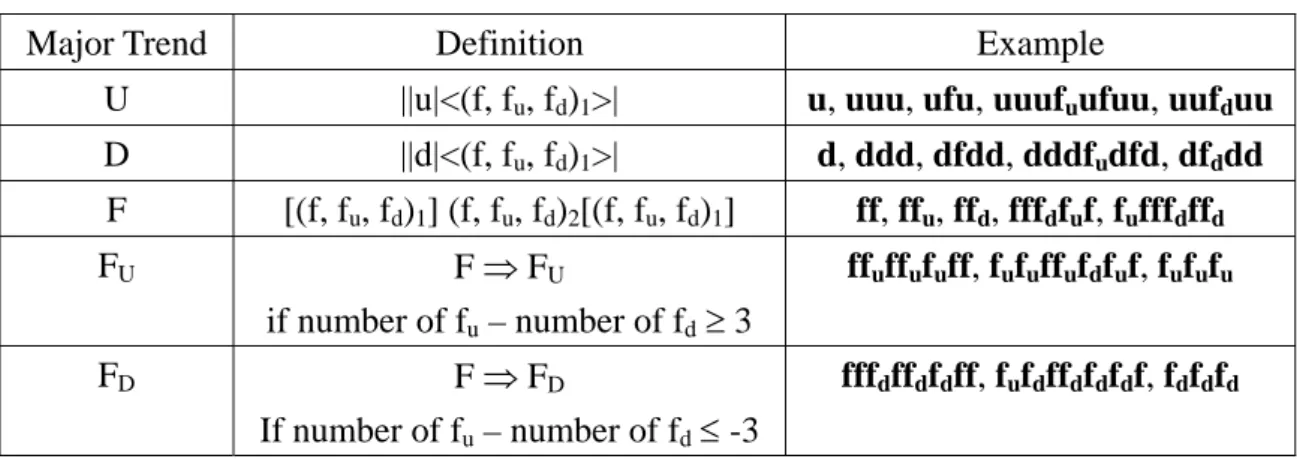
Table 3-2 The summarization of major trends
Major Trend Definition Example
U ||u|<(f, fu, fd)1>| u, uuu, ufu, uuufuufuu, uufduu
D ||d|<(f, fu, fd)1>| d, ddd, dfdd, dddfudfd, dfddd F [(f, fu, fd)1] (f, fu, fd)2[(f, fu, fd)1] ff, ffu, ffd, fffdfuf, fufffdffd FU F ⇒ FU if number of fu – number of fd ≥ 3 ffuffufuff, fufuffufdfuf, fufufu FD F ⇒ FD If number of fu – number of fd ≤ -3 fffdffdfdff, fufdffdfdfdf, fdfdfd
The time series already transformed via EPLR is further represented by a sequence of major trends to perform a rough match first. The idea of major trends match is already shown in Figure 3-8. Each major trend should match with another major trend with the same feature, namely, U should match with U, D should match with D and F is not allowed to match with U or D. However, it is not the only kind of match that a sequence of major trends matches with exactly the same sequence of major trends. Major trends F, FU and FD are capable of matching with each other for
the reason that FU and FD are two special kinds of F and should be much similar to F.
Besides, FU is allowed to match with U and FD is allowed to match with D because we
don’t want any possible miss and they both represent up or down. The following are our matching rules for each major trend:
Def 5:
1. U: U, FU, Mix of U & FU
2. D: D, FD, Mix of D & FD
3. F: F, FU, FD
For instance, U can match with U, FU and Mix of U & FU, such as UFUU.
Example: Consider a sequence of major trends, DFUDFUFDD, which is the same as
the following sequences of major trends: 1. DFDFUFD
2. DUDFUFD 3. DFDFUD 4. DUDFUD
For simplicity, we do not make any difference among F, FU and FD. In the above
four sequences of major trends, F can be replaced by FU or FD, so any subsequence
which is the same as the above four sequences can be matched.
3.3.2 Level-2 Detailed Subsequence Match
As shown in Figure 3-8, one major trend only matches with another major trend. Each major trend has to calculate the distance with the major trend it matches and the distance is called a major trend distance. Then the final distance between a query and a subsequence which is similar to query is the sum of all major trend distance. The following is the formal definition:
Def 6:
Given two time series Q and S, they are major trends matched sequences of the same length r, where:
Q = {qt1, qt2, …, qti, …, qtr}
S = {st1, st2, …, sti, …, str}
qti and sti are ith major trend of Q and S.
The ith major trend distance is noted as MTD(qti, sti) and the distance between S and
Q, Dist(S, Q), is computed in Eq. (5)
∑
= r MTD qti sti
Q S
An asymmetric distance function modifying DTW is used to compute the major trend distance based on query because our concern is that how subsequences similar to query but not how query similar to subsequences. Considering two times series Q and S, a distance function is asymmetric if the distance between Q and S, Dist(Q, S), is distinct from the distance between S and Q, Dist(S, Q). We called this DTW-based distance function Modified DTW (MDTW) to discriminate from original DTW. We allow expanding and compressing the time axis to provide a better match, but the each element of query needs to match and is always compared once. The only consideration is how the shape of the matched subsequence is similar to query. We do not want the length or noise of the matched subsequence affect the result of similarity matching, so the number of compared elements is fixed to the number of elements contained in query. That is, every element in the query should be matched. In our application, time is not an issue because the data needed to calculate is localized. Segments in a major trend are much less than the whole time series. The definition of distance function MDTW is as follows:
Def 7:
Given two time series Q and S, of length n and m respectively, where:
Q = {q1, q2, …, qi, …, qn}
S = {s1, s2, …, sj,…, sm}
Let D(i, j) be the minimum distance of matching between (q1,q2, …, qi) and (s1,s2, …,
sj), the MDTW distance can be computed as in Eq. (6)
D (i, j) = min{ distmdtw(qi, sj)+D(i-1, j-1), distmdtw(qi, sj)+D(i, j-1), D(i-1, j) } (6)
Figure 3-11 MDTW Algorithm
An algorithm used by dynamic programming for MDTW distance is given in Figure 3-11. An example is also shown in Figure 3-12. One thing should be noticed that although the step-patterns are the same for DTW and MDTW, one of the directions have a little different meaning. Due to the definition that each query element only compares one time, the right direction of warping path means that query skips one element to compare with next element. In Figure 3-12, the cells underlined mean these elements are skipped and their distances are not included in the final distance. The mapping example of DTW and MDTW is described in Figure 3-13 and Figure 3-14, respectively. As we can see in Figure 3-13 and Figure 3-14, there are three time series Q, S1 and S2, where Q = {6, 1, 6, 7, 1}, S1 = {2, 7, 1, 7, 2, 1, 1} and S2 = {4, 3, 6, 1}. It is obvious that Q is more similar to S1 than to S2. Let us consider distance function of DTW and MDTW, respectively. DTW(S1, Q) = 7 and DTW(S2, Q) = 5. Instead of our intuition, the distance between S1 and Q is more than the distance between S2 and Q for comparing every element. As for MDTW, MDTW(S1, Q) = 2 and MDTW(S2, Q) = 5. The result is more reasonable because some elements are skipped to find if the shape is similar to Q.
Figure 3-12 Example of MDTW Figure 3-13 Mapping of DTW Figure 3-14 Mapping of MDTW
the subsequence similarity.
Def 8: Given two subsequences Q and S which are both represented by EPLR, Q and
S are similar if they satisfy the following two conditions:
1. Major trends of Q and S match with each other.
2. Dist(Q,S) < γ where Dist(Q,S) is the sum of all major trend distances as computed in Eq. (5) and γ ≥ 0 is user-specified parameter.
In our definition of subsequence similarity, the first condition can be referred to as an index quickly to check and filter out a lot of time series which are not qualified. Our experiment shows that major trends match is reliable on the ground truth acquired by DTW. The second condition makes sure which one is truly similar and Dist(Q,S) can be a basis of ranking.
Chapter 4
Experimental Results
In this chapter, we evaluate the performance of the proposed subsequence similarity matching mechanism. As for implementation environment, all the programs are implemented in Java SE 6 and run on hardware with Intel Pentium 4 CPU 1.6 GHz with 512 Mbytes memory and software with Windows XP Professional Version 2002 system. The experimental results include two parts. In section 4.1, the experimental validation of EPLR is shown by clustering and classification. In section 4.2, we demonstrate the similarity retrieval is effective and efficient.
4.1 Experiments of EPLR
Keogh et al. [31] introduced two methods, clustering and classification, to evaluate similarity measure. Lin et al. [21] also utilized these two methods to validate their Symbolic Aggregate approXimation (SAX) representation. Here, we verify the reliability of EPLR by these two methods.
4.1.1 Clustering
Clustering is one of the most common data mining tasks. The Cylinder-Bell-Funnel data set which consists of three classes is shown in Figure 4-1. The goal of clustering is to separate each class in Figure 4-1 into a cluster, time series in each class respectively, such as (1), (2) and (3) in a cluster and (4), (5) and (6) in another cluster. We experiment clustering on 20 datasets with class labels known (data
randomly chosen. Each cluster has a centroid and each time series in a cluster has a distance with the centroid of its cluster. If the distance between a time series and the centroid in the same cluster is larger than the distance with the centroid of another cluster, the time series is move to that cluster. The final result is received when we do not need to change clusters anymore. We compute the distance with two methods to experiment which one can get better clustering results. One is raw data with Euclidean distance and the other one is EPLR with Manhattan distance. We only compare the difference of angles of segments. The data overlap of EPLR is set to 1/2. We will show overlapping 1/2 segment size is much reliable in later experiments. Since EPLR allows dimensionality reduction by defining how many data points k generate a segment, the experiments are run on different size of a segment and the best one is reported. k is experimented from 16 × 20 up to 16 × 25
if k does not exceed n/2, where
n is the length of time series.
Figure 4-1 The Cylinder-Bell-Funnel data set
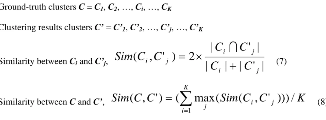
To evaluate the clustering results, an approach is needed to show whether the clustering results are good or not. [35] and [36] introduces a similarity measure between two clusters as follows:
Ground-truth clusters C = C1, C2, …, Ci, …, CK
Clustering results clusters C’ = C’1, C’2, …, C’j, …, C’K
Similarity between Ci and C’j,
|
'
|
|
|
|
'
|
2
)
'
,
(
j i j i j iC
C
C
C
C
C
Sim
+
×
=
I
(7)Similarity between C and C’,
Sim
C
C
Sim
C
C
K
K i j i j
(
(
,
'
))
)
/
max
(
)
'
,
(
1∑
==
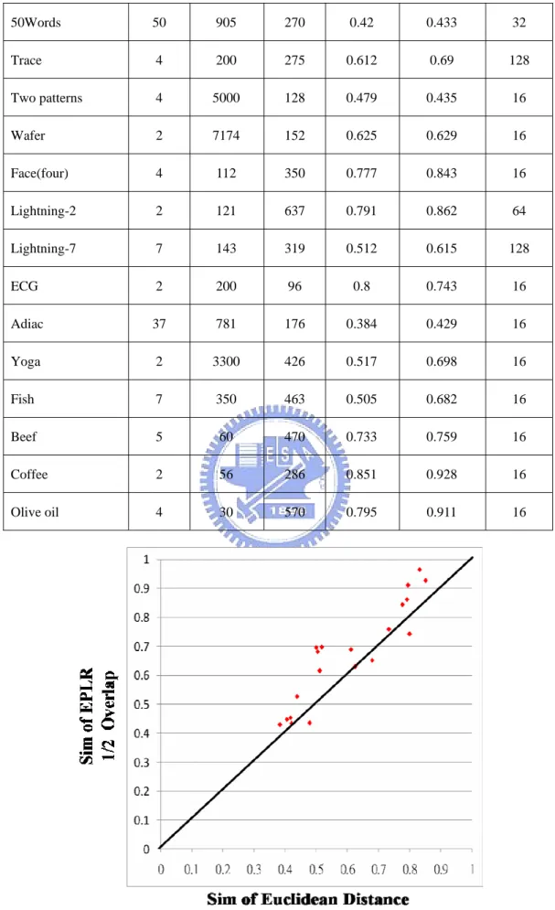
(8)Here, we use the symbol Sim to represent the similarity measure between two clusters. Sim is equal to 0 if two clusters are completely different and Sim is equal to 1 if two clusters are identical. The comparison of Sim over 20 datasets is shown in Table 4-1. For clarity about the comparisons, the Sim for each data set is plotted in a 2-dimensional plan in Figure 4-2. The x-axis represents the Sim of Euclidean distance and the y-axis represents the Sim of EPLR with 1/2 overlapping. If a point is located at the lower triangle, then Euclidean distance is more accurate than that of the EPLR with 1/2 overlapping and vice versa for the upper triangle. Because the results of K-Means change with cluster centroids chosen initially, K-means is executed fifty times and the best result is reported.
Table 4-1 Comparison of Sim
Data Sets Number of Classes Size of Data Set Time Series Length Sim of Euclidean Distance Sim of EPLR 1/2 Overlap Segment Size k Synthetic Control 6 600 60 0.679 0.652 16 Gun-point 2 200 150 0.5 0.696 16 CBF 3 930 128 0.832 0.965 32
50Words 50 905 270 0.42 0.433 32 Trace 4 200 275 0.612 0.69 128 Two patterns 4 5000 128 0.479 0.435 16 Wafer 2 7174 152 0.625 0.629 16 Face(four) 4 112 350 0.777 0.843 16 Lightning-2 2 121 637 0.791 0.862 64 Lightning-7 7 143 319 0.512 0.615 128 ECG 2 200 96 0.8 0.743 16 Adiac 37 781 176 0.384 0.429 16 Yoga 2 3300 426 0.517 0.698 16 Fish 7 350 463 0.505 0.682 16 Beef 5 60 470 0.733 0.759 16 Coffee 2 56 286 0.851 0.928 16 Olive oil 4 30 570 0.795 0.911 16
Distance
In this experiment, we examine that our method is better than raw data with Euclidean distance because most datasets are located at upper triangle. However, the results of K-Means are affected a lot by cluster centroids chosen initially, so we further use classification to verify the reliability EPLR.
4.1.2 Classification
Classification of time series has attracted much interest from the data mining community. To demonstrate the advantage of EPLR, the 1-nearest neighbor algorithm proposed by Keogh et al. [31] is used with following methods. Raw data with Euclidean distance, PLR with a similarity measure for PLR [37], PAA with Manhattan distance and EPLR with Manhattan distance (no, 1/3, 1/2 overlap). The similarity measure for PLR processes the time series first by breaking some segments at a point which corresponds to an endpoint in the other time series and then compute the Manhattan distance of both endpoints of each segment. For PAA, the equal length of each segment is set to 16 which is the best segmentation in our application. The 1-NN algorithm is evaluated by using leaving-one-out. In the first place, given a database of labeled time series, the database is partitioned into two sets, one is called training set and the other one is called testing set. Then the leaving-one-out is applied to each time series in testing set. That is, the class label of time series in testing set is regarded as unknown and is assigned the class label of its nearest neighbor in training set, based on a distance function defined. It is a hit if the class label is the same as the original class label, or it is a miss. The error rate is defined in Eq. (9).
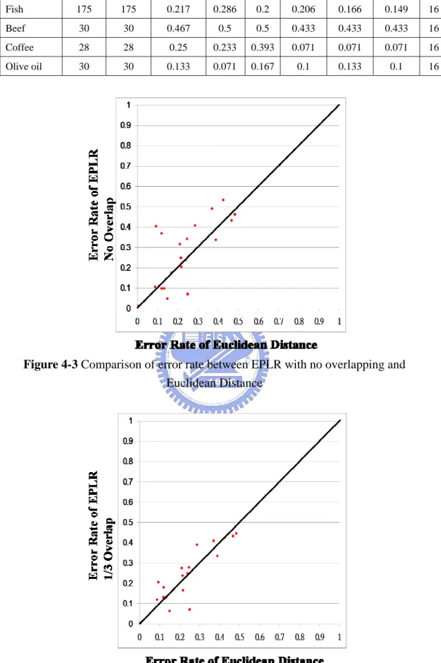
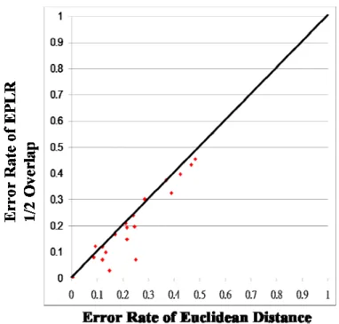
clarity in the comparisons, the error rate for each data set is also plotted in a 2-dimensional plan. Assume the x-axis represents the error rate of Euclidean distance and the y-axis represents the error rate of EPLR with 1/2 overlapping. In contrast to clustering results, if a point is located at the lower triangle, then EPLR with 1/2 overlapping is more accurate than that of Euclidean distance. Error rates of Euclidean distance and EPLR with no overlapping, EPLR with 1/3 overlapping and EPLR with 1/2 overlapping are shown in Figure 4-3, Figure 4-4 and Figure 4-5, respectively. Error rates of EPLR with 1/2 overlapping and PAA and PLR are also illustrated in Figure 4-6 and Figure 4-7, respectively.
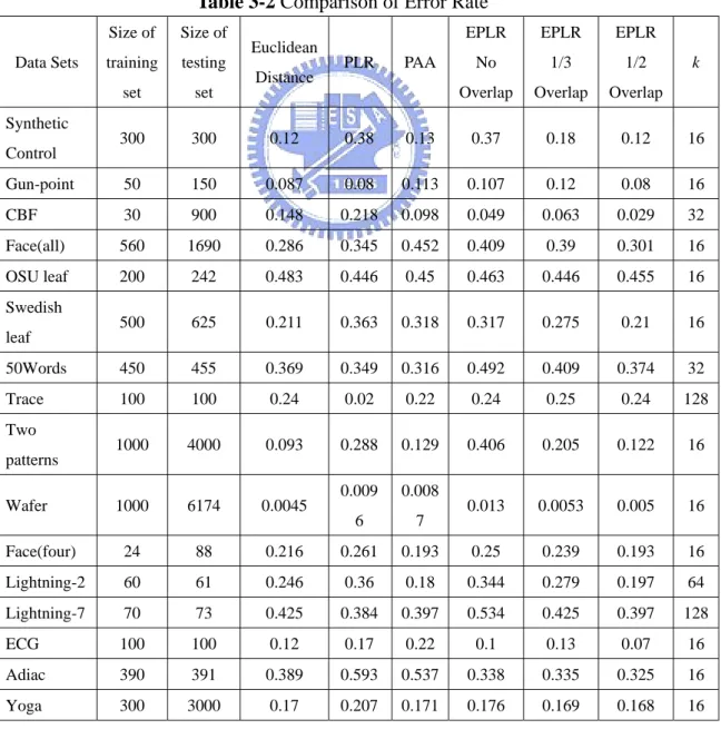
Table 3-2 Comparison of Error Rate
Data Sets Size of training set Size of testing set Euclidean Distance PLR PAA EPLR No Overlap EPLR 1/3 Overlap EPLR 1/2 Overlap k Synthetic Control 300 300 0.12 0.38 0.13 0.37 0.18 0.12 16 Gun-point 50 150 0.087 0.08 0.113 0.107 0.12 0.08 16 CBF 30 900 0.148 0.218 0.098 0.049 0.063 0.029 32 Face(all) 560 1690 0.286 0.345 0.452 0.409 0.39 0.301 16 OSU leaf 200 242 0.483 0.446 0.45 0.463 0.446 0.455 16 Swedish leaf 500 625 0.211 0.363 0.318 0.317 0.275 0.21 16 50Words 450 455 0.369 0.349 0.316 0.492 0.409 0.374 32 Trace 100 100 0.24 0.02 0.22 0.24 0.25 0.24 128 Two patterns 1000 4000 0.093 0.288 0.129 0.406 0.205 0.122 16 Wafer 1000 6174 0.0045 0.009 6 0.008 7 0.013 0.0053 0.005 16 Face(four) 24 88 0.216 0.261 0.193 0.25 0.239 0.193 16 Lightning-2 60 61 0.246 0.36 0.18 0.344 0.279 0.197 64 Lightning-7 70 73 0.425 0.384 0.397 0.534 0.425 0.397 128 ECG 100 100 0.12 0.17 0.22 0.1 0.13 0.07 16 Adiac 390 391 0.389 0.593 0.537 0.338 0.335 0.325 16
Fish 175 175 0.217 0.286 0.2 0.206 0.166 0.149 16 Beef 30 30 0.467 0.5 0.5 0.433 0.433 0.433 16 Coffee 28 28 0.25 0.233 0.393 0.071 0.071 0.071 16 Olive oil 30 30 0.133 0.071 0.167 0.1 0.133 0.1 16
Figure 4-3 Comparison of error rate between EPLR with no overlapping and Euclidean Distance
Figure 4-5 Comparison of error rate between EPLR with 1/2 overlapping and Euclidean Distance
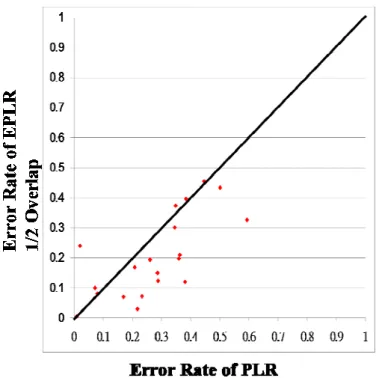
Figure 4-7 Comparison of error rate between EPLR with 1/2 overlapping and PAA Our experiments demonstrate that data overlapping is necessary. Besides, overlapping 1/2 data of previous segment is good enough to beat Euclidean distance. We do not need more data overlap because it can cause more overhead. The comparisons between EPLR and PAA and PLR are also shown that EPLR is superior to PAA and PLR in most of the data sets.
4.2 Experiments of EPLR Similarity Retrieval
Since the superiority of EPLR is proven, the following experiments are all based on EPLR. In this section, we use pruning rate, miss rate and CPU cost to test our similarity retrieval. Pruning rate refers to efficiency that how many time series pruned by major trends match. In order to verify effectiveness, we compare the time series matched by major trends and the ground truth is acquired by DTW distance applied to
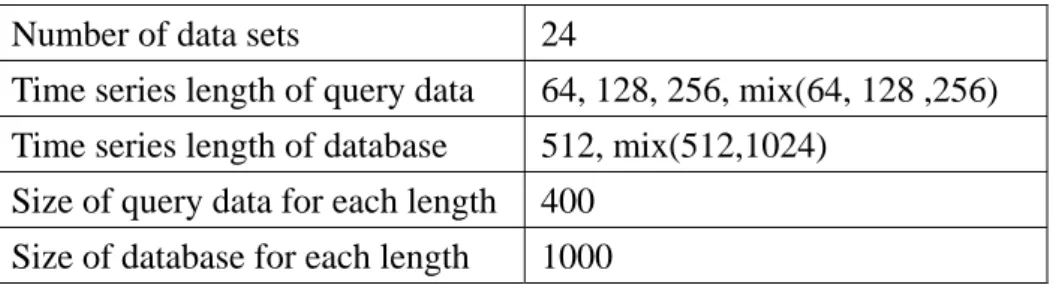
Euclidean distance and the proposed method without major trends match. The experimental results are presented based on 24 data sets out of 32 benchmark data sets used in [22]. Table 4-3 shows the parameter settings for 24 data sets. The symbol mix( ) means mix the items in ( ).
Table 4-3 Parameter settings for 24 data sets
Number of data sets 24
Time series length of query data 64, 128, 256, mix(64, 128 ,256) Time series length of database 512, mix(512,1024)
Size of query data for each length 400 Size of database for each length 1000
Each data set contains query data and database data and the length of query data is less than the length of database data. Before experimenting, there are still some parameters needed to define. Parameters a and b in Def 3 for major trends match are set to 0.4 and 0.2. For simplicity, each time series is divided into equal segments with 16 data points. We define a DTW distance threshold ε as a ground truth for similarity. Each time series in query data and each time series in database have a minimum subsequence distance, called MSSD. ε is set to 1/5 of average MSSD. Figure 4-8, 4-9, 4-10 and 4-11 show the results of four combinations of different length of query data and database, respectively. In Figure 4-8, the length of query data is 64 and the length of database is 512. We change the length of query data to 128 and 256 in Figure 4-9 and Figure 4-10. In Figure 4-11, we mix the length of 64, 128 and 256 for query data and the length of 512 and 1024 for database. As for CPU cost, two data sets, Fetal ECG and Power Data, are chosen to compare. CPU cost of Fetal ECG is shown in Figure 4-12 and CPU cost of Power Data is described in Figure 4-13.
Table 4-4 Summarization of pruning rates and miss rates for different length of data
64-512 64-512 128-512 128-512 256-512 256-512 mix-mix mix-mix ballbeam 15.76 0 31.33 0 32.37 0.17 22.94 0.05 ballon 13.45 0 24.86 0 38.87 0.2 21.08 0.03 power_data 12.73 0.1 23.75 0.5 56.8 0.6 26.71 0.01 network 3.64 0 15.04 0 22.99 0 16.17 0 chaotic 12.46 1.1 54.82 1.3 93.18 1.4 45.49 0.6 cstr 9.52 0 16.35 0 32.52 0.007 15.78 0 dryer2 28.65 0.03 25.68 0.005 41.8 0.07 28.51 0.04 eeg 14.04 0.1 61.83 0.2 95.65 1.1 50.09 0.1 ERP_data 9.52 0 23.24 0 39.7 0.6 20.66 0 evaporator 13.38 0 22.83 0 33.43 0 19.9 0 foetal_ecg 25.82 0.007 55.57 0.5 79.31 0.7 50.78 0.8 koski_ecg 9.12 0 23.74 0.09 55.38 1 22.54 0.05 ocean 3.05 0 13.07 0.49 38.01 3.1 12.57 1 pHdata 18.61 0.04 27.99 0.05 49.04 0.2 30.94 0.03 powerplant 13.34 0 33.74 0.9 62.25 1 30.04 0.3 random_walk 9.32 0 40.95 0.7 80.96 1.3 31.2 0 robot_arm 14.5 0 31.1 0.03 57.75 1.1 28.58 0.05 shuttle 4.23 0 10.72 0 21.07 0.2 10.21 0 soiltemp 15.54 0 35.07 0.1 50.67 1 27.62 0.2 steamgen 17.11 0.07 32.23 0.6 43.73 1.2 26.04 0.1 sunspot 11.13 0 42.55 0.4 86.12 1 42.07 0.4 tide 17.63 0 75.43 0.1 97.76 2.9 58.52 0.5 winding 21.85 1.2 60.74 2.88 81.55 3.5 49.97 1.8 wool 24.46 0 28.42 0.002 48.11 0.5 25.21 0.05
Figure 4-8 Pruning rate and Miss rate withlength of query = 64, and length of time series in Database = 512
Figure 4-9 Pruning rate and Miss rate with length of query = 128, and length of time series in Database = 512
Figure 4-10 Pruning rate and Miss rate with length of query = 256, and length of time series in Database = 512
Figure 4-11 Pruning rate and Miss rate with length of query = mix of 64, 128, 256 and length of time series in Database = 512
Figure 4-12 CPU cost of Fetal ECG between Euclidean Distance, Proposed Method and MDTW
Figure 4-13 CPU cost of Power Data between Euclidean Distance, Proposed Method and MDTW
Observe that the miss rates of all data sets are low enough for different length of query. The miss rate rises a little only on the condition that the pruning rate is too high, such as tide and winding in Figure 4-10. Besides, the results indicate that pruning rates are quite satisfactory for most data sets. By Figure 4-12 and Figure 4-13, we can further prove that our proposed method is much faster than Euclidean distance. Even
Chapter 5
Conclusion and Future Work
5.1 Conclusion of Our Proposed Work
In this thesis, we proposed a subsequence similarity retrieval mechanism to deal with the shape-based similarity. A new representation EPLR is presented and for similarity retrieval, a similarity measure for EPLR is proposed. EPLR is a kind of segmentation technique, divides a time series of the length n into m segments with equal length k. Each segment overlaps parts of data with previous segment and is represented by the angle of its best-fit line segment. Since segments are equally split and presented by angles, there are many advantages, such as easy to implementation, retaining information of trends and dimensionality reduction. Experimental results show that the representation EPLR not only reduces the dimension but is also reliable to handle shape or trend of time series. In contrast with PLR and PAA, EPLR is superior to them.
We define 2-level similarity measure based on EPLR. On first level, the major trends of two subsequences have to be matched because if two time series are similar, their shape should be similar. We can prune a lot of non-qualified time series to speed the retrieval. We assign each segment a segment trend in accordance with its angle. Then a merge mechanism is applied to segment trends to form major trends. After that, we can perform major trends match by specific rules. As regards to the second level, the distance of two subsequences which is the sum of all major trend distance must
conditions are met. Experiments demonstrate that the pruning rate of our similarity measure is satisfactory with acceptable miss rates and CPU cost is of the proposed method is low enough.
5.2 Future Work
Our work uses angles as the representation of shape or trend of time series and the similarity retrieval based on this representation is discussed. There is an extended research on applying EPLR to other data mining tasks such as anomaly detection and motif discovery. As for EPLR, how many data points in a segment is highly data dependent. We may analyze the data distribution to decide the number of data points in a segment. Furthermore, only the trends but not the real values of data are concerned in the work. It may be possible to combine the real values with angles to make the similarity retrieval more robust and powerful.
Bibliography
[1]. R. Agrawal, C. Faloutsos, and A. R. Swami, Efficient Similarity Search Databases, Proceedings of the 4th International Conf. Foundations of Data Organization and Algorithms (FODO), pp. 69-87, 1993.
[2]. R. Agrawal and R.Srikant, Mining Sequential Patterns, Proc. of 11th IEEE Intel. Conf. on Data Engineering (ICDE), pp. 3-14, Mar. 1995
[3]. D.J. Berndt and J.Cliford, Using Dynamic Time Warping to Find Patterns in Time Series. AAAI-94 Workshop on Knowledge Discovery in Databases, pp.350-370, 1994.
[4]. C. Faloutsos, M. Ranganathan, and Y. Manolopoulos, Fast Subsequence Matching in Time-Series Database, Proc. of the ACM SIGMOD Intel. Conf. on Management of Data, pp. 419-429, 1994.
[5]. G. Das, D. Gunopulos, and H.Mannila, Finding Similar Time Series, Proc. of Principles of Data Mining and Knowledge Discovery, 1st (PKDD), Pages 88-100, 1997.
[6]. K-P. Chan and A. Fu, Efficient Time Series Matching by Wavelets, Proc. of the 15th IEEE Intel. Conf. on Data Engineering (ICDE), pp. 126-133, 1999.
[7]. B.-K. Yi, H.V. Jagadish, and C.Faloutsos, Efficient Retrieval of Similar Time Sequences under Time Warping, Proc. of the 14th IEEE Intel. Conf. on Data Engineering (ICDE), pp. 201-208, 1998.
[8]. K-P. Chan, A. Fu, and C. Yu, Haar Wavelets for Efficient Similarity Search of Time-series: With and Without Time Warping, Journal of Transactions on