線狀液晶光學圖像形成之研究

國

立

交

通

大

學

光電工程研究所

博

士

論

文

線狀液晶光學圖像形成之研究

Study on the Optical Pattern Formation through

Nematic Liquid Crystal Films

研究生：徐旭寬

指導教授：王淑霞 教授

賴暎杰 教授

線狀液晶光學圖像形成之研究

Study on the Optical Pattern Formation through

Nematic Liquid Crystal Films

研究生: 徐旭寬 Student: Hsu-Kuan Hsu 指導教授: 王淑霞 教授 Advisor: Prof. Shu-Hsia Chen

賴暎杰 教授 Prof. Yinchieh Lai

國

立

交

通

大

學

電

機

資

訊

學

院

光

電

工

程

研

究

所

博

士

論

文

A Dissertation

Submitted to Institute of Electro-Optical Engineering College of Electrical Engineering and Computer Science

National Chiao Tung University in Partial Fulfillment of the Requirements

for the Degree of Doctor of Philosophy

in

Electro-Optical Engineering June 2004

Hsinchu, Taiwan, Republic of China

線狀液晶光學圖像形成之研究

研究生: 徐旭寬

指導教授: 王淑霞 教授

賴暎杰 教授

國立交通大學光電工程研究所

摘 要

近十年來，非線性光學系統中光學圖像形成的研究吸引了很多學者 投入心思探討。在這些研究中，理論的分析和模擬大致可以分為兩大類 的光學系統，一為被動系統，一為光學共振腔系統；本論文將針對被動 非線性光學系統中的光學圖像形成加以探討。被動光學系統指的是由外 場驅動的光學系統，理想來說是穩定且固定的，並沒有考慮到例如光學 共振腔中的居數反轉的現象。由於外場和非線性材料的作用，在系統存 在微擾或雜訊時，透過強大的非線性作用，外場原本的狀態會受到雜訊 的微擾而變得不穩定，因而造成光學圖像的產生。 在本論文中，我們探討利用外加似靜電場偏壓的線狀液晶在單一光 回饋的系統中，其光學圖像形成的特性，雖然在此單一光回饋系統中光 學圖像形成的穩定和控制已有很多的研究，但是線狀液晶基本的物理特 性對於此光學圖像形成的現象影響尚未有深入的探討。在以往利用線狀 液晶做此類研究的文獻中，據我們所知並無考慮電場效應的影響，是故 我們針對在外加電壓偏壓下的線狀液晶其本身物理非等向特性，研究此 光學圖像形成現象的影響。在理論分面，我們根據線狀液晶連續體理 論，藉由系統最低能量的 Euler-Lagrange 分析步驟過程中推導出液晶分子

在外場條件下的橫向分佈之擴散方程，根據此擴散方程，我們可以明顯 看出液晶本身的彈性非等向性會造成擴散方程中擴散長度的非等向性； 針對此系統的擴散方程作線性穩定性分析，我們可以得到光學圖像形成 所需的臨界入射光強度，分析此臨界光強我們發現擴散長度的非等向性 也會造成臨界光強在橫截面分佈的非等向特性。在外加電場偏壓下的線 狀液晶樣品，由於其本身的介電非等向性，液晶分子的排列可以利用外 加電場加以適當地控制。在理論分析中，我們發現擴散長度和系統的非 線性強度會和液晶分子的分佈有關。 所以，考慮液晶的彈性非等向性及液晶分子分佈的可電調特性，我 們提出了不外加傅立葉空間濾波器的條件下，利用液晶本身非等向性造 成臨界光強度非等向的特性，簡單地控制入射光強，即可得到條狀和六 角狀的光學圖像。此外，由於彈性非等向性會造成臨界光強分佈的非等 向性，所以我們更針對液晶法蘭克彈性常數的相對值對此光學圖像之形 成會有哪些更進一步的影響作更深入的理論分析。另一方面，由於系統 的非線性強度會和液晶分子的分佈有很大的關係，所以我們也就外加偏 壓對系統非線性強度的影響作了進一步的分析。考慮電壓和臨界光強度 非等向分佈的特性，我們更提出了在適當單一入射光強下，藉由電壓控 制系統的非線性強度調變臨界光強的分佈曲線，也可以得到條狀和六角 狀的光學圖像的證據。 在理論分析中我們所提出的圖像形成特性，不論是利用控制入射光 強或是電壓調變臨界光強分佈的方法，皆可以實驗加以印證。我們的實 驗結果也可定性的和理論分析相符。

Study on the Optical Pattern Formation through

Nematic Liquid Crystal Films

Student: Hsu-Kuan Hsu Advisor: Prof. Shu-Hsia Chen Prof. Yinchieh Lai

Institute of Electro-Optical Engineering

National Chiao Tung University

Abstract

Optical pattern formation in nonlinear optical systems has been widely studied in the last decade. Analysis and simulations of pattern formation in two classes of systems are presented. These are passive systems and the cavity systems. Here, we focus on the pattern formation in passive nonlinear optical systems. Passiveness means that the excitation is driven by anexternally field, smoothly and constantly in the ideal case, rather than through population inversion. Optical pattern formation results from the nonlinear interaction between the external field and the nonlinear materials. Once a perturbation exists in this nonlinear system, such as the scattering light or the noise, the initial state of the external field may be perturbed and become unstable through the high nonlinearity of the system.

In this dissertation, we investigate the optical pattern formation phenomena by using the quasi-static electric-field-biased liquid crystal

(NLC) films in combination with the one-feedback-mirror system proposed by Firth and Pare. Though the controlling and stabilizing methods have been widely studied the basic physical uniqueness of the nematic liquid crystals appeared in these optical pattern formation phenomena has not been explored very clearly. The governing diffusion-like equation of the optical field induced phase variation in the transverse plane used in most theoretical analysis is assumed to be isotropic based on Firth’s method. However, the diffusion-like equation should be modified when nematic liquid crystals are used. Unlike the previously used operating modes such as the hybrid-aligned films, the vertically aligned films or the liquid crystal light valve (LCLV) samples, we further consider the parallelly planar-aligned NLC films biased by a quasi-static electric field. To our knowledge, the electric field effect on the optical pattern formation phenomena has not been included in the earlier theoretical analysis. From our previous works, we know that the optical nonlinearity of such NLC films can be effectively modulated by suitably applying a quasi-static electric field.

Therefore, considering the anisotropic properties of the nematic liquid crystals, we derive the governing diffusion-like equation for the optical field induced phase variation in the transverse plane. Furthermore, the threshold intensity distribution for the patterns to be formed is also derived by the results of the linear stability analysis (LSA) of the governing diffusion-like equation. By analyzing the anisotropic threshold intensity distribution we propose a possible method to obtain the roll and the hexagon patterns without canceling the anisotropic property of the threshold intensity. We successfully observe the roll and the hexagon patterns by simply controlling the input light intensity. Furthermore, from the theoretical analysis, we know that the anisotropic distribution of the

threshold intensity results from the elastic anisotropy of the nematic liquid crystals. Hence, we analyze the issue of how the elastic anisotropy affects the optical pattern formation phenomena. From the results of the analysis of the effects of the elastic anisotropy, we further study the influence of the applied electric field. The nonlinearity of the system can, indeed, be modulated by the applied electric field through the modulation of the orientation of the liquid crystal molecules electrically. Therefore, a simple electric-method is achieved to obtain different optical patterns with a single input light intensity. The experimental results in our work qualitatively agree with the theoretical results well and the suggested pattern-forming properties in our theoretical analysis can be reasonably proved.

致謝

不知不覺在交大已是第六個年頭, 此時此刻也將為博士生求學生涯劃下一個句 點。鳳凰花開, 和風徐徐, 伴著我邁向人生的下一個階段。求學階段中苦樂交織, 感謝我的雙親徐添貴先生與胡秀銀女士, 長久以來給予我支持與鼓勵, 也讓我無 後顧之憂的完成我的學業。 感謝我敬愛的大姊, 二姊和姊夫, 無時無刻的為我打 氣。家人的支持與鼓勵是我完成學業的最大支柱, 謝謝你們。 踏進交大, 多年來在我的指導教授王淑霞老師的教導下讓我於人生的課題上得到 許多的啟發, 不僅僅是在專業的學術領域研究上讓我有更深入的了解, 更重要的 是王老師的一字一句與諄諄教誨對我為人處世有深刻的影響。 感謝您,我人生的 導師 ! 感謝傅永貴教授, 是您帶我進入了光學的世界, 感謝賴暎杰教授, 您親切的指導讓 我能堅持下去。 感謝大師兄吳俊傑教授, 大師姊梁寶芝教授, 有了你們的建議與 幫忙, 我才得以完成我的論文。 李偉教授, 感謝您在我低潮時都適時拉了我一把, 您的鼓勵感懷於心。 實驗室的眾多學長姊, 同學和學弟妹們, 謝謝你們讓我的研究生生活充滿了挑戰 和歡樂。毓仁學長, 慶逸學長, 伯綸學長, 立宜學長, 秋蓮學姊感謝你們給了我很 多寶貴的意見與協助。 景翔學長, 勇勳學長, 仰恩學長, 鵲如學姊, 志成學長感謝 你們讓我能很快適應研究生的生活。我的同學們菱芝, 傅丞, 建賢感謝你們給我 快樂的研究生活與回憶。 怡欣, 您長久來的鼓勵是我非常感激的。佳成, 信全, 乾煌, 揚宜, 彥廷, 梓傑, 朝旭, 惠雯, 英豪, 德源, 建宏, 世郁, 美琪, 品發, 庭毅, 瑞傑 謝謝你們豐富了我的研究生活。 勇兒, 夏青, 庭瑞, 葦俐謝謝你們長久以來的照 顧和關懷, 有你們的鼓勵讓我堅持下去完成我的論文。范姜, 舒展我志同道合的 學弟們, 謝謝你們! 俊雄, 怡安, 芝珊學姊謝謝你們幫了我很多忙, 讓我在最後 的關鍵時刻可以專心完成工作。

感謝我生命中的好友知己們, ouch, 正桑, 小莉, 逸凱, blue, daff 謝謝你們的鼓勵, 最後, 感謝我生命中最重要的伴侶, 筱慧, 謝謝你一路陪著我, 陪我哀傷, 陪我快樂, 一直以來都默默付出與承受, 感謝您~

新竹國立交通大學

Table of contents

Abstract (in Chinese) i

Abstract (in English) iii

Acknowledgement (in Chinese) vi

Table of Contents vii

List of Figures and Tables x

List of Symbols xv

Chapter 1 Introduction ………. 1

1-1 Overview ………... 1

1-1-1 Types of liquid crystals ………. 1

1-1-2 The thermotropic liquid crystals ………... 2

1-2 Nonlinear optics ……… 5

1-2-1 General overview of nematic-optical nonlinearities ………….. 6

1-2-2 Optical pattern formation in passive nonlinear optical systems 7 1-3 A survey of the optical pattern formation observed in a nematic liquid crystal film in one-feedback-mirror system ……… 9

1-4 Aim of the research ……….. 10

Chapter 2 Theory ……….. 12

2-1 Field-induced optical phase variation in the transverse plane when an electric-field-biased liquid crystal film is used ………... 12

2-2 The threshold intensity for patterns to be formed ……… 19

3-1 Anisotropic threshold intensity distribution results from the

elastic anisotropy of nematic liquid crystals ………. 25

3-2 Influence of Frank elastic constant anisotropy on optical pattern formation phenomena ………... 28

3-3 Analysis of the influence of dielectric anisotropy of nematic liquid crystals on optical pattern formation phenomena ………….. 40

Chapter 4 Experiments ……… 44

4-1 Sample preparation, experimental setup and measurements ……… 44

4-2 Experimental observations ………... 46

4-2-1 Optical pattern formation in a parallelly planar-aligned NLC film ………. 46

4-2-2 Obtaining different optical patterns by the optical method … 48 4-2-3 Obtaining different optical patterns by the electric method … 50 Chapter 5 Discussion and Conclusions ………... 54

5-1 Discussion ……… 54

5-1-1 Discussion about the observed patterns obtained by the optical method

………...

54

5-1-2 Discussion about the observed patterns obtained by the electrical method ………. 56

5-1-3 Overall discussion ………... 58

5-2 Conclusions and future works ……….. 59

Appendix I ………. 64

List of Figures and Tables

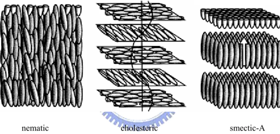
Chapter 1

Fig. 1.1 The schematic molecules arrangement of nematics, cholesterics and smectic-A liquid crystals.

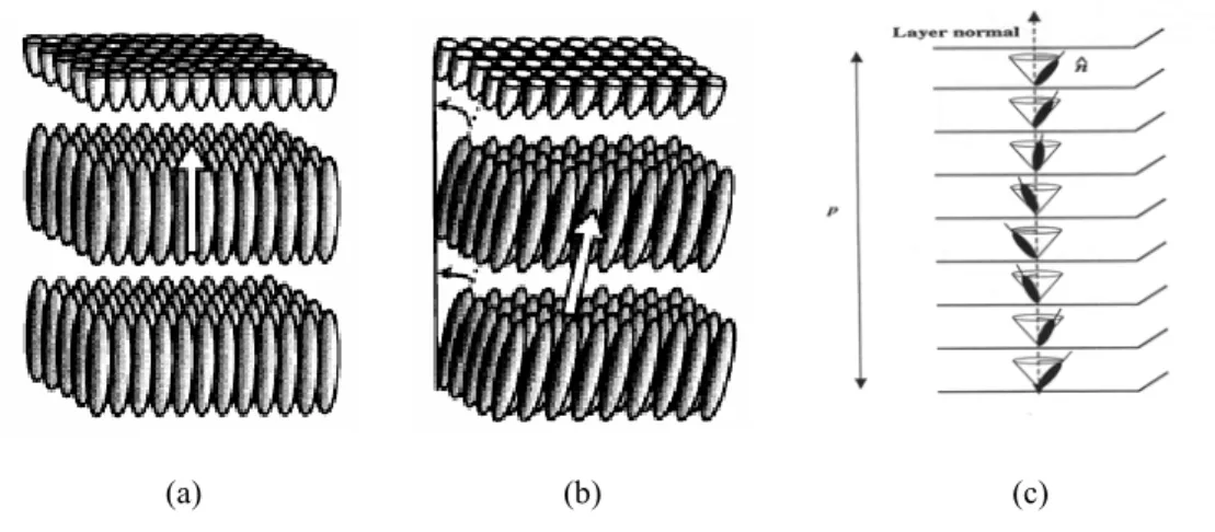
Fig. 1.2 The schematic molecules arrangement of smectic-A, smectic-C and smectic-C* liquid crystals.

Chapter 2

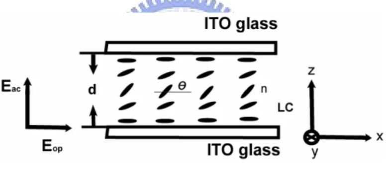
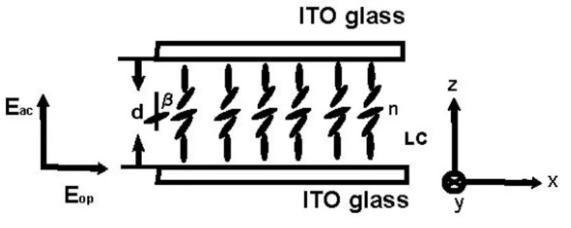
Fig. 2.1 The planar-aligned nematic liquid crystal cell: LC, liquid crystal; θ, molecular orientational angle; Eop , optical field; Eac, electric

field; , molecular director; d, cell thickness, and ITO, indium tin oxide.

nˆ

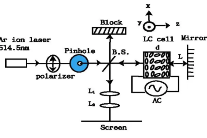
FIG. 2.2 Geometric scheme of the one-feedback-mirror system: B.S., beam splitter; d, cell thickness; L, feedback length; LC, liquid crystal; L’i, lens.

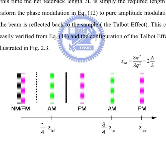
Fig. 2.3 The transferring between the phase modulation and amplitude modulation based on the Talbot Effect (Ztal: Talbot length).

Fig. 2.4 The vertically-aligned nematic liquid crystal cell: LC, liquid crystal; β, molecular orientational angle; Eop , optical field; Eac,

electric field; n , molecular director; d, cell thickness, and ITO,

indium tin oxide.

ˆ

Chapter 3

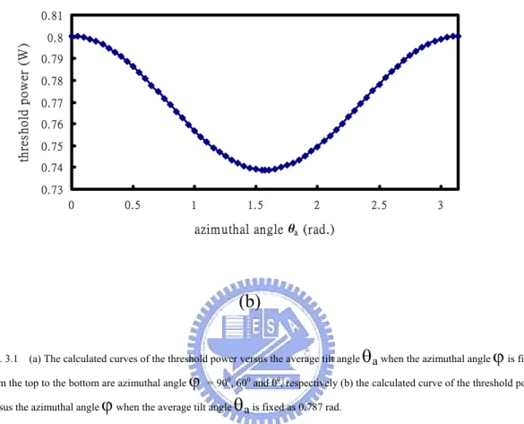
Fig. 3.1 (a) The calculated curves of the threshold power versus the average tilt angle θa when the azimuthal angle ϕ is fixed; from

the top to the bottom are azimuthal angle ϕ = 900_{, 60}0 _{and 0}0_,

respectively (b) the calculated curve of the threshold power versus the azimuthal angle ϕ when the average tilt angle θa is

fixed as 0.787 rad.

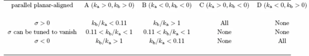
Table 3.1 Classification of regions according to the Frank elastic constant anisotropy.

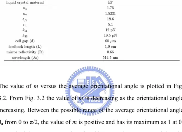
Table 3.2 The liquid crystal parameters, cell properties, and optical system parameters used in the calculations

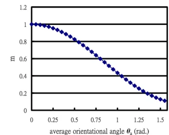
Fig. 3.2 The calculated value of m versus the average orientational angle θa.

Fig. 3.3 The calculated effective diffusion anisotropy σ versus the elastic anisotropies. (a) for region A; with ka = 1.5 (b) for region B; with ka = −0.5.

Fig. 3.4 The calculated diffusion lengths versus the average tilt angle θa.

(a) for region A; with ka = 1.5 (b) for region B; with ka = −0.5.

Please note that lx is the same for different kb/ka if ka is not

changed.

Fig. 3.5 (a) The calculated diffusion lengths versus the average tilt angle θa (b) The calculated threshold intensity versus the average tilt

angle θa when the azimuthal angle ϕ is fixed (c) The calculated

threshold intensity versus the azimuthal angle ϕ when the average tilt angle θa is fixed With ka = 0.625, kb/ka = 0.512

Fig. 3.6 (a) The calculated threshold intensity versus the average tilt angle θa when the azimuthal angle ϕ is fixed; with ka = 0.625, kb/ka =

−0.4. (b)The calculated threshold intensity versus the average tilt angle θa when the azimuthal angle ϕ is fixed with ka = −0.2, kb/ka

= −1.

Fig. 3.7 (a) The calculated curve of the average tilt angle θa versus the

biasing voltage (b) the effective nonlinear coefficient α versus the average tilt angle θa; with beam diameter=1.4 mm, d=68 µm,

Fig. 3.8 (a) the calculated threshold power distribution for different θa;

from the top to the bottom are θa = 0.6, 0.75 and 0.9 rad,

respectively (b) the calculated threshold power distribution for different θa; from the bottom to the top are θa = 0.9, 1.05 and

1.2 rad, respectively; with beam diameter=1.4 mm, d=68 µm, L=1.9 cm, R=0.65, input light power=0.91 W.

Chapter 4

Fig. 4.1 Experimental setup: B.S., beam splitter; d, cell thickness; L, feedback length; LC, liquid crystal; L’i, lens.

Fig. 4.2 Conoscopic picture for the planar aligned NLC sample.

Fig. 4.3 Near-field patterns observed on the screen; input power=0.83 W, biased voltage=1.117 Vrms, d=68 mm, L=1.9 cm, R=0.65, beam diameter=1.4 mm,and exposure time=1.25 ms.

Fig. 4.4 Stable roll patterns observed on the screen (a) input power=0.74 W (b) input power=0.78 W

Fig. 4.5 Pattern sequence showing the competition between the roll and the hexagon patterns; input power=0.8 W.

Fig. 4.6 Stable hexagon and chaotic patterns observed on the screen (a) input power= 0.83 W (b) input power= 0.98 W

Fig. 4.7 Observed picture when the biasing voltage is zero with input light power= 0.91 W

Fig. 4.8 Stable hexagon patterns observed on the screen (a) V= 1.117 Vrms

(b) V= 1.114 Vrms

Fig. 4.9 Stable roll patterns observed on the screen; with V= 1.032 Vrms

Fig. 4.10 Pattern sequence showing the competition between the roll and the hexagon patterns; V= 1.096Vrms.

Chapter 5

Fig. 5.1 The calculated curve of the threshold power versus the azimuthal angle ϕ when the average tilt angle θa is fixed at about 0.787

radian and the biased voltage is 1.117 Vrms.

Fig. 5.2 The calculated curves of the threshold power versus the azimuthal angle φ, from the bottom to the top are biased voltage=1.114 Vrms and 1.032 Vrms, respectively; the horizontal

line indicates the input light power=0.91 W; with beam diameter=1.4 mm, d=68 µm, L=1.9 cm, R= 0.65.

List of Symbols

nˆ

molecular director

P polarization of vector form E electric field of vector form

χ(i) _{susceptibility of i-th order}

n refractive index NLC nematic liquid crystal LCLV liquid crystal light valve LSA linear stability analysis

θ orientation of liquid crystal molecules

ne, no extraordinary and ordinary refractive indices

ε//, ε⊥ dielectric constants, parallel and perpendicular to molecular

director d cell thickness ITO indium tin oxide L feedback length

f total free energy density

fd free energy density for elastic deformation fe free energy density for electric term

k11 splay elastic constant k22 twist elastic constant k33 bend elastic constant

D electric displacement of vector form H magnetic field of vector form

B magnetic induction of vector form

k k =(k₃₃/k₁₁)−1

k* k*=(k11/k33)-1

w w=1−ε// /ε⊥

µ

µ=1−(ne/no)2

I input light intensity

a

θ

average tilt angle

p

θ

optically modulating amplitude

t

θ

transverse orientational angle in the middle layer of the liquid crystal cell

γ

_{viscosity coefficient}

V root mean square value of the biased voltage li diffusion length in the i direction

) 2 ( _t

i

J θ Bessel function of the first kind of order i fr

th

V Freedericksz voltage

neff effective index of refraction

τ response time )

, ( yx

δφ Kerr induced optical phase variation α effective nonlinear coefficient

ρ perturbation amplitude E0 incident plane wave

Ef optical beam just after the NLC film q wave-vector

ϕ

azimuthal angle

Eb reflected beam on the NLC film

r mirror reflectance

u spatial frequency in the x direction v spatial frequency in the y direction

u0 spatial frequency of the phase grating in the x direction v0 spatial frequency of the phase grating in the y direction

Λx phase grating spatial period in the x direction Λy phase grating spatial period in the y direction

a

β average polar angle

ka ka=(k33/k11)−1 ka* ka*=(k11/k33)−1

kb kb=(k22/k11) − 1 kb* kb*=(k22/k33) − 1

σ effective diffusion anisotropy parameter

m a a a J J m θ θ θ ) (2 ) 2 ( 2 1 ( 2 1 ₁ 0 − + = ) R mirror reflectivity

Chapter 1 Introduction

1-1 Overview

In this dissertation, liquid crystals are classified by utilizing the classification scheme of De Gennes and Prost [1], and we will give a brief description of thermotropic liquid crystals. Furthermore, the optical properties of nematics are mentioned briefly.

1-1-1 Types of liquid crystals

Liquid crystals are beautiful and unique materials. The term liquid crystal signifies a state that is intermediate between the crystalline solid and the amorphous liquid. As a rule, a substance in this state is strongly anisotropic in some of its properties and yet exhibits a certain degree of fluidity. The first observations of liquid crystalline or mesomorphic behavior were made towards the end of the nineteenth century by Reinitzer [2] and Lehmann [3] (mesomorphic: of intermediate form). Several thousands of organic compounds are known now to form liquid crystals. An essential requirement for mesomorphism to occur is that the molecule must be highly geometrically anisotropic in shape, like a rod or a disc. Depending on the detailed molecular structure, the system may pass through one or more mesophases before it is transformed into the isotropic liquids. Transitions to these intermediate states may be brought about by thermal processes (thermotropic mesomorphism) or by the influence of solvents (lyotropic mesomorphism). Therefore, utilizing the classification scheme of liquid crystal by P. G. De Gennes and J. Prost [1],

there are four major types of liquid crystals: (i) thermotropic, (ii) lyotropic, (iii) polymer and (iv) amphiphilic compounds.

Among these four types, the molecules of the thermotropic liquid crystals are small organic molecules, either rod-like or disk-like, for which an amphiphilic character may or may not be crucial. The simplest way to induce a transition is to vary the temperature therefore they are commonly called thermotropic. Lyotropic liquid crystals are made up of two or more components. Generally, one of them is an amphiphile and another is water. A familiar example of such a system is soap in water. Here the temperature effects are difficult to control, and the nature parameter which one can adjust to induce phase transition is the concentration of the components. Lyotropic liquid crystals are receiving increasing scientific and technological attention because of the way they reflect the unique properties of their constituent molecules. Considering the main-chain or side-chain polymers that are thermotropic mesogens, aside from temperature the molecule weight may also be considered as a variable. Polymeric liquid crystals are potential candidates for electronic devices and ultra-high-strength materials. Amphiphilc compounds may give rise to associations and to mesomorphic behavior, either in the presence of selective solvent or as a pure phase. Thus, depending upon which of the above conditions holds, amphiphilic compounds may be lyotropic or thermotropic.

1-1-2 The thermotropic liquid crystals

well as the nonlinear optical properties are thermotropic liquid crystals. In this dissertation, only thermotropic materials are concerned. Thermotropic liquid crystal phases are observed in pure compounds and mixtures. As the temperature increases, these compounds go through a series of phase transitions: from solid to liquid crystal, to isotropic liquid, and finally to vapor phase. Following the nomenclature proposed originally by Friedel [4], thermotropic liquid crystals are classified broadly into three types: nematic, cholesteric and smectic, as shown in Fig. 1.1.

nematic cholesteric smectic-A

Fig. 1.1 The schematic molecules arrangement of nematics, cholesterics and smectic-A liquid crystals

The nematic phase has a high degree of long-range orientational order of the molecules, but no long-range translational order. The aligned nematic liquid crystal molecules, on the average, are characterized by one symmetry axis, call the director . The direction of is arbitrary in space and the state of director and - are indistinguishable. The director can be reoriented by an external field, such as electric field, magnetic field or optical field.

nˆ nˆ

nˆ nˆ

except for the chial-induced twist in the directors, as shown in Fig. 1.1. This property results from the synthesis of cholesteric liquid crystals; they are obtained by adding a chiral molecule to a nematic liquid crystal. Some materials, such as cholesteric esters, are naturally chiral. The helical structure can result in selective reflection in wavelength and circular polarizations. The polarization states of the reflected and transmitted waves depend on the pitch length of the cholesteric. Cholesteric liquid crystals have found important applications in areas such as laser cavity mirrors, color filters, and polymer dispersed cholesteric liquid crystal displays.

Smectic liquid crystals, unlike nematic, possess positional order; that is, the positions of the molecules are correlated in some ordered pattern. Form the structure point of view, all smectics are layered-structured with a well-defined interlayer spacing. Therefore, smectics are more ordered than nematics. For a given material, smectic phases usually occur at temperature below the nematic domain. Several subphases of smectics have been discovered, in accordance with the arrangement or ordering of the molecules and their structural symmetry properties. Here, we only briefly describe basic structures of smectic A, C, and C* phases as shown in Figs. 1.2(a)-(c).

The scheme diagram of layered structure of a smectic-A liquid crystal is shown in Fig. 1.2(a). In each layer the molecules are positionally random, but directionally ordered with their long axis normal to the layer normal. The system is optically uniaxial and the optical axis is normal to the plane of the layer.

(a) (b) (c)

Fig. 1.2 The schematic molecules arrangement of smectic-A, smectic-C and smectic-C* _{liquid crystals}

The smectic-C phase is a tilted form of smectic-A, i.e., the molecules are inclined with respect to the layer normal. (cf. Fig. 1.2(b)). The smectic-C* liquid crystals, as depicted in Fig. 1.2(c), is an interesting class of liquid crystal materials. The structure of smectic-C* is similar to that of smectic-C except for a helical tilt distributions from layer to layer. Another exciting feature of smectic-C* phase is that it exhibits ferroelectricity. Using this spontaneous polarization, a bistable LC modulator with microsecond response time has been demonstrated in a ferroelectric liquid crystal (FLC) cell.

1-2 Nonlinear optics

All optical phenomena occurring in a material arise from the optical field induced polarization P. In the electromagnetic theory of light, the material response to the illumination of light is described by the following equation:

where P is the induced polarization of the material, E is the electric field of the light and , and are the first-, second- and third-order susceptibilities, respectively. For low light intensity, the high order terms are very small and the optics is adequately described by the first term E. Linear optics is described by which is related to the

index of refraction by n ) 1 ( χ _χ(2) _χ(3) ) 1 ( χ _χ(1)

2_{=1+ . For the early days without laser light}

sources, the scientist can not obtain a reasonable nonlinear effect since a high intensity and coherent light source is required. In 1961, an early second harmonic generation experiment gave the first experimental confirmation for nonlinear theories. A ruby laser with a wave length at 0.6943μm was focused on the front surface of a crystalline-quartz plate. The emergent radiation was examined with a spectrometer and was found to contain radiation at twice the input light frequency.

) 1 ( χ

After the early second-harmonic generation experiments, the field of nonlinear optics has grown rapidly. Many different nonlinear optical phenomena have been observed. These include wave mixing, optical phase conjugation, stimulated scattering, optical pattern formation etc. As indicated above, these nonlinear optical phenomena require intense laser beam. The intensity requirements become even more stringent for higher order process.

1-2-1 General overview of nematic-optical nonlinearities

In linear optical process the physical properties of nematic liquid crystals, such as the molecular structure, the individual or collective molecule

orientation, the temperature, the density, the population of the electric levels, and so on, are not affected by the optical fields. The optical properties of nematics can be controlled by some external electric fields; this gives rise to a variety of electro-optical effects which are widely used in many electro-optical displays and image-processing applications.

Nematic liquid crystals are also optically nonlinear materials since their physical properties (molecular orientation, temperature and density) are easily perturbed by such an applied high-intensity optical field. Since commonly used liquid crystal molecules are dielectric anisotropic, a polarized light from a laser can induce a realignment of the molecules in the ordered phase. This results in a change of the index of refraction. Other commonly occurring mechanisms that give rise to the changes of the refractive index are laser-induced changes in the temperature and the density. These changes can arise from several mechanisms. Elevation in the temperature is a natural consequence of the photo-absorptions and the subsequent processes. In the nematic phase the index of refraction is highly dependent on the temperature, through their dependence of on the order parameters, as well as the density.

1-2-2 Optical pattern formation in passive nonlinear optical

systems

Optical pattern formation in nonlinear optical systems has been widely studied in the last decade. Analysis and simulations of pattern formation in two classes of systems are presented. These are passive systems and the cavity systems. Here, we focus on the pattern formation in passive

nonlinear optical systems. Passiveness means that the excitation is driven by an externally field, smoothly and constantly in the ideal case, rather than through population inversion. Optical pattern formation results from the nonlinear interaction between the external field and the nonlinear materials. Once a perturbation exists in this nonlinear system, such as the scattering light or the noise, the initial state of the external field may be perturbed and become unstable through the high nonlinearity of the system.

After the instability analysis made by Firth and Pare [5] and the experimental observation of hexagon patterns made by Grynberg [6] using the sodium vapor as the nonlinear material, the optical pattern formation phenomena under two counter-propagating pump-beams condition have been confirmed. In 1990, Firth further proposed and demonstrated the optical pattern formation by using a simple arrangement which places a thin Kerr medium in front of a planar feedback mirror [7]. Using this simple one-feedback-mirror system numerous experiments have been successfully performed by using different materials as the nonlinear medium, such as the atomic vapor, the photorefractive crystals and the liquid crystals. The hexagons are the usual patterns frequently observed in these experiments. To stabilize and select patterns other than the hexagons, one can add a Fourier filter in the feedback route [8-10] or break the rotational symmetry by applying the anisotropic nonlinear medium [11]. Up to now, the use of the liquid crystal light valve combined with a Fourier filter in the feedback route is the most favored choice [12].

1-3 A survey of the optical pattern formation in a nematic

liquid crystal film in one-feedback-mirror system

Utilizing the one-feedback-mirror mirror system the observation of optical pattern formation by using liquid crystals as the nonlinear materials has been studied for many years. In 1992, R. Macdonald and H. J. Eichler successfully observed the hexagon patterns by using a hybrid-aligned nematic liquid crystal (NLC) cell [13]. In the next year, E. Santamato used a clinic-positioned vertical-aligned NLC cell to perform the experiment and also observed the hexagon patterns [14, 15]. Furthermore, in 1994, Santamato observed the roll patterns by considering the unequal property in the diffusion lengths of the governing diffusion-like equation for this system [11]. By rotating the sample to reduce the anisotropy of the diffusion lengths Santamato obtained the hexagon patterns. Furthermore, by inserting a slit as a filter in the feedback route he also obtained the square-like patterns.

In 1995, using the photosensitive-electrode-coated liquid crystal light valve (LCLV), T. Tschudi performed a detailed study on the pattern formation phenomena [16]. In recent years, Tschudi paid more efforts at the stabilizing and pattern selecting topics by adding a Fourier filter in the feedback route [10, 12]. On the other hand, Santamato successfully observed the optical patterns in a defocusing Kerr-like film by adding dye materials into the nematic materials since in the past time one always obtained the optical patterns in a focusing material [17].

1-4 Aim of the research

In this dissertation, we investigate the optical pattern formation phenomena by using the quasi-static electric-field-biased liquid crystal (NLC) films in combination with the one-feedback-mirror system proposed by Firth.

Though the controlling and stabilizing methods have been widely studied, the basic physical uniqueness of the nematic liquid crystals appearing in these optical pattern formation phenomena has not been explored very clearly. The governing diffusion-like equation of the optical-field-induced phase variation in the transverse plane used in most theoretical analysis is assumed to be isotropic based on Firth’s method. However, as Santamato mentioned in Ref. 11, the diffusion-like equation should be modified and is anisotropic when nematic liquid crystals are used. Unlike the previously used operating modes, such as the hybrid aligned films, the vertically aligned films or the LCLV samples, we further consider the parallelly planar-aligned NLC films biased by a quasi-static electric field. To our knowledge, the electric field effect on the optical pattern formation phenomena has not been included in the theoretical analysis. From our previous works, we know that the optical nonlinearity for such NLC films can be effectively modulated by suitably applying a quasi-static electric field [18-20].

Therefore, considering the anisotropic properties of the nematic liquid crystals we derive the governing diffusion-like equation for the optical-field-induced phase variation in the transverse plane and the threshold intensity distribution for the patterns to be formed is also

derived by the results of the linear stability analysis (LSA) of the governing diffusion-like equation. By analyzing the anisotropic threshold intensity distribution we propose a possible method to obtained the roll and the hexagon patterns without canceling the anisotropic property of the threshold intensity as Santamato did in Ref. 11. We successfully observe the roll and the hexagon patterns by simply controlling the input light intensity [21].

With the results obtained in Ref. 21, we know that the anisotropic distribution of the threshold intensity is resulted from the elastic anisotropy of the nematic liquid crystals. Therefore, we analyze the issue of how the elastic anisotropy affects the optical pattern formation phenomena [22]. From the results we get in Ref. 22, we further study the influence of the applied electric field. The nonlinearity of this system indeed can be modulated by the applied electric field through the modulation of the orientation of the liquid crystal molecules electrically. Therefore, a simple electric-method to obtain different optical patterns is achieved with a single input light intensity [23].

In the following chapter, a general theoretical description of the governing diffusion-like equation and the analytical results of the threshold intensity for both the parallelly planar-aligned and the vertical-aligned NLC films are presented. In chapter 3, we give a discussion of how the intrinsic anisotropic properties affect the optical pattern formation phenomena. The experimental results concerning a parallelly planar-aligned NLC film are given in chapter 4. Finally, the discussion and conclusion are made in chapter 5.

Chapter 2 Theory

In this chapter, the general theoretical derivation of the governing diffusion-like equation for the optical-field-induced phase variation and the analytical results of the threshold intensity for the optical pattern formation for both the parallelly planar-aligned and the vertical-aligned NLC films are presented.

2-1 Field-induced optical phase variation in the transverse

plane when an electric-field-biased liquid crystal film is

used

In order to obtain the governing diffusion-like equation for the optical-field-induced phase variation the governing diffusion-like equation for the orientational distribution of the liquid crystal directors in the transverse plane with externally applied fields must be obtained first. We start from the continuum theory for the NLCs. If one assumes a p-polarized light beam impinges on an electric-field-biased liquid crystal film, then the liquid crystal directors will be reorientated when the electric and the optical fields are high enough. As the liquid crystal directors are reorientated, the light beam passing through the liquid crystal film will experience a phase delay according to the orientational distribution of the liquid crystal directors. Therefore, the orientational

distribution of the liquid crystal directors θ(x, y, z) must be calculated first.

Fig. 2.1 shows the configuration of the quasi-static electric-field-biased planar-aligned homogeneous NLC film considered in our derivation and Fig. 2.2 shows the geometric scheme of our one-feedback-mirror system for observing the optical pattern formation phenomena. The nematic material is assumed to have positive optical and dielectric anisotropies, namely ne > no and

ε

// >

ε

⊥ where n and

ε

denote the refractive

indices and dielectric constants, and the subscripts refer to the directions parallel and perpendicular to the director, respectively.

Fig. 2.1 The planar-aligned nematic liquid crystal cell: LC, liquid crystal; θ, molecular orientational angle; Eop ,

optical field; Eac, electric field; nˆ , molecular director; d, cell thickness, and ITO, indium tin oxide.

A quasi-static electric field is applied along the z-axis and is perpendicular to the unperturbed director . A p-polarized light impinges on the NLC film with its polarization direction parallel to the easy axis of the liquid crystal directors. After it passing through the NLC sample the light propagates freely to and from the planar feedback mirror and finally impinges on the sample again.

Fig. 2.2 Geometric scheme of the one-feedback-mirror system: B.S., beam splitter; d, cell thickness; L, feedback length; LC, liquid crystal; L’i, lens

In order to obtain the governing diffusion-like equation for the optical field induced phase variation in the transverse plane the orientational distribution of the molecules θ(x, y, z) should be calculated first. From the continuum theory, which is a macroscopic phenomenological theory of liquid crystals dealing with a slowly varying director field, the orientational distribution function θ(x, y, z) is obtained by minimizing the total free energy F dv. The total free energy density f for our system is

∫

= f f = fd + fe +fop , (1) where fd = [ ( ˆ) (ˆ ˆ) (ˆ ˆ) ] 2 1 2 33 2 22 2 11 n k n n k n n k ∇• + •∇× + ×∇× , fe = − _π Ee•De 8 1 _, and fop= [ ] 8 1 op op op op D H B E • + • − π ,

terms, respectively. In these relations, k11, k22 and k33 are the splay, twist,

and bend elastic constants, respectively. E and D represent the electric field and displacement while H and B are the magnetic field and induction, respectively. Therefore, choose the coordinate system with the z axis perpendicular to the cell walls, the x-y plane coincides with the input cell wall and the direction is along with the easy axis of the liquid crystal directors. Considering the director = (cosθ, 0, sinθ) the

free energy density f can be expressed as

xˆ

nˆ )] )( ( cos sin 2 ) )( sin 1 ( ) )( cos 1 [( { 2 1 2 2 2 2 11 z x k z k x k k f ∂ ∂ ∂ ∂ + ∂ ∂ + + ∂ ∂ + = θ θ θ θ θ θ θ θ _{2 2 1/2} 2 2 22 ) sin 1 ( ) sin 1 ( 8 } ) ( θ µ θ πε θ − − − − ∂ ∂ + ⊥ c In w D y k z e , (2) where k =(k₃₃/k₁₁)−1 , w=1−ε///ε⊥ , , is the z

component of the electric displacement, c is the velocity of light in vacuum, and I is the input optical intensity. Actually, it’s not easy to deal with the three dimensional equation directly. Instead of solving the distribution function θ(x, y, z) by the Euler–Lagrange equations directly, we assume a trial solution of θ(x, y, z) as

2 ) / ( 1− ne no = µ D_z

)

sin(

)]

,

(

[

)

,

,

(

d

z

y

x

z

y

x

θ

_a

θ

_p

π

θ

=

+

) sin( ) , ( d z y x t

π

θ

= . (3)

We also assume the hard-boundary condition, θ(z = 0)=θ(z = d)= 0. Here d is the thickness of the sample and

θ

a,

θ

p, and

θ

t represent the

electrically biased spatial average orientational angle, the optically modulated amplitude, and the transverse orientational angle in the middle layer of the liquid crystal cell, respectively. Substituting Eq. (3) into Eq. (2), integrating the total volume of the cell, and following the Euler- Lagrange optimization process, we can get the torque balance equation of the liquid crystal directors. After some algebra and considering the viscositic term, the torque balance equation can be expressed as

G J k I I V V y l x l t t fr th t t y t x t _]2 (2 ) 2 [ ) ( ) ( 1 2 2 2 2 2 2 2 2

θ

θ

_θ

θ

θ

γ

+ = − + ∂ ∂ − ∂ ∂ − ∂ ∂ , (4) with ]} ) 2 ( ) 2 ( 2 1 [ 2 1 { ) ( 1 ₁ 0 2 2 t t t x J J k d G l θ θ θ π + + − = , ) ( ) ( 1 11 22 2 2 k k d G l_y

π

= _,

)]}

2

(

)

2

(

[

2

2

{

k

k

J

_{0 t}

J

_{2 t}

G

=

+

−

θ

−

θ

_, 2 1 // 11 _] [ 2 ⊥ − =

ε

ε

π

π

k V_{th ,} and ) ( 1 ) ( 2 11

_µ

π

e fr ck _{d n} I − = _{. (5)}

Here

γ

is the viscosity coefficient, V is the root-mean-square value of the biased voltage, li (i = x, y) is the diffusion length in the i direction,

) 2 ( t i

J θ is the Bessel function of the first kind of order i, and and are the Freedericksz optical intensity and voltage. From Eq. (4), one can see that the viscosity term indicates the dynamic behavior of the orientation of NLC directors. Furthermore, the spatial orientation of NLC directors is also related with the spatial distribution of the external fields. Eq. (4) can be changed into the diffusion-like equation for the optical phase variation in the transverse plane since the effective index of refraction for the NLC materials can be expressed as

fr

I

th

V

₍

₁

_sin

2

₎

2 2

θ

µ

−

=

e eff

n

n

_{, (6)}

and the optical phase variation in the transverse plane is

Ψ

=

∫

d eff

dz

n

y

x

0 0

2

)

,

(

λ

π

. (7)

After substituting Eq. (3) into Eq. (6) and replacing in Eq. (7) by Eq. (6), the diffusion-like equation can be expressed as

eff

n

_I

I

S

T

V

V

y

l

x

l

t

th fr y x

_∂

+

Ψ

=

−

+

Ψ

∂

−

∂

Ψ

∂

−

∂

Ψ

∂

]

[

₂ 2 2 2 2 2 2 2

τ

_{. (8)}

Here

τ

is the response time related with the viscosity coefficient, S and T are the coefficients which are functions of the material parameters and the orientation of the liquid crystal directors. Now if we consider a uniform applied voltage, then the phase variation in the transverse plane directly comes from the light intensity variation in the transverse plane. It follows that the constant phase terms and the constant driving forces can be removed from Eq. (8). Therefore a simplified governing diffusion-like equation for the Kerr-induced optical phase variation δφ( yx, ) can be obtained and shown as

I y l x l t x y

δφ

αδ

δφ

δφ

δφ

τ

+ = ∂ ∂ − ∂ ∂ − ∂ ∂ 2 2 2 2 2 2 ; (9) G I J dJ n fr a t e 0 1 1(2 ) (2 ) 2

λ

θ

θ

µ

π

α

= − _{. (10)}

Eq. (9) is similar to the equation proposed by Firth in Ref.7 except the anisotropic property of the diffusion lengths in the transverse plane and α is the effective nonlinear coefficient affected by the molecular orientations as shown in Eq. (10). From Eq. (5) and Eq. (10), we can see that the relative coefficients can be obtained as the material parameters, the electrically biased spatial average orientational angle

θ

a, and the optically modulating amplitude

θ

p are known. The electrically biased spatial average orientational angle

θ

a can be determined by minimizing

the total free energy under the hard boundary condition and the assumption of a uniformly distributed electric field. Following the Euler-Lagrange optimization process, we find that

θ

_a has to obey the following equation ) 2 ( 2 ) 4 ( )]} 2 ( ) 2 ( 2 [ 2 2 { _{2 1} 2 2 0 a fr th a a a J k I I V V J J k

_θ

_θ

_θ

θ

+ − + = − + _{. (11)}

Eq. (11) can be calculated numerically if d, V, I, and the material parameters are all known. From our previous paper [22], the optically modulating amplitude is much smaller than the electrically biased spatial average orientational angle, . Therefore we can reasonably substitute

a

p θ

θ <<

t

θ

by

θ

_a in both Eq. (5) and Eq. (10).

2-2 The threshold intensity for patterns to be formed

To obtain the threshold intensity for patterns to be formed, we follow the linear stability analysis (LSA) in Ref. 11. Consider the geometric scheme shown in Fig. 2.2. The incident plane wave passes through the NLC film then propagates freely to and from the reflecting mirror and finally impinges on the NLC film. For such a system, the LSA of Eq. (9) can be performed by assuming that a noise with its azimuthal angle ϕ on the transverse plane interacts with the input plane wave . The noise and interfere with each other which results in the optical intensity

0 E 0 E 0 E

distribution on the transverse plane. Since the NLC molecules possess the dielectric anisotropic property, the orientation of the NLC molecules follows the distribution of the optical intensity. Therefore, when the plane wave passes through the NLC film the plane wave experiences a phase modulation. Now assume a small sinusoidal phase modulation

0

E

δφ

is applied to the forward plane wave . After the plane wave just passes through the sample, it will experience the phase variation as given by 0 E E₀ x y q ϕ

]}

)

sin

(

)

cos

cos[(

1

{

)

,

(

x

y

E

₀

i

q

x

q

y

E

_f

=

+

ρ

ϕ

+

ϕ

=

E

0

{

1

+

i

δφ

}

. (12)

Here

ρ

<<

1

is the perturbation amplitude and the terms related to the wave vector q have been written in the polar form with the azimuthal angle

ϕ

from the axis of the anisotropy to the wave vector clockwise. The beam then propagates freely to and from the reflecting mirror. This part of wave propagation can be readily modeled by the Fresnel propagation formula such as

) ,

( yx

_∫∫

− = e e ( ) E ( y ( e ( dx z y E j y j j z jkz λ π λ π λ π _{+ + +} ' ' ) ' ,' ) , , ( ' )' 2 ) ' '2 2 2 2 dy e x z j x z x y xx yy f x z λ ]} ) [( )] , ( 2 ) , ( 2 ) , ( {[ } )] ( 2 1 {[ } )] ' ' cos( 1 [ { } ) ' ,' ( { ) ( 0 0 0 0 ) ( 0 ) ' ' ( )' ' ( )' ' ( ) ( 0 ) ' ' ( ' ' 0 ) ( ) ' ' ( ) ( 2 2 2 2 2 2 ' ' ' ' 2 2 2 2 2 2 2 2 2 2 v u z j y x z j jkz y x z j y q x q j y q x q j y x z j jkz y x z j y x y x z j jkz y x z j t y x z j jkz e z j v v u u i v v u u i v u e z j e E e e e i F e z j e E e y q x q i E F e z j e e y x U F e z j e y x y x + − + + + − + + + + + + ⊗ − − + + + + (13) where , 1 ; 1 ; 1 ; 1 ; sin 2 ; cos 2 0 0 y x y y x x v u y v x u q q q q Λ = Λ = = = = Λ = = Λ =

π

ϕ

π

ϕ

here u0 and v0 are the spatial frequencies of the phase grating in the x and

y directions, respectively. Λx and Λy are the spatial period of the grating in

the x and y directions, respectively. Then the reflected beam on the film can be expressed as (14) = + + = + + πλ λ π λ π λ π λ π λ π λ π λ π λ ρ ρ δ λ ρ λ ρ λ λ = = )}, cos( 1 { )]} ( 2 cos[ 1 { ]} ) [( )] , ( 2 ) , ( 2 ) , ( {[ 2 2 2 0 2 0 2 2 2 2 4 0 0 0 ) ( 0 ) ( 0 0 0 0 ) ( _{i i} e π ρ ρ 0 y q x q e i e E y v x u e i e E e z j v v u u v v u u v u e z j E y x q z j jkz v u z j jkz v u z j y x z j jkz + + + + ⊗ − − + + + + = − + − + − + π πλ πλ πλ λ ρ π ρ λ δ λ = =

)].

cos(

(

_x

_y

_rE

_i

4

_x

_q

_y

E

,

,

2

)

=

[

1

ρ

π2

+

_y 2 2 2 0

e

e

q

L

_x q L j L jk b

+

− πλ

By squaring the reflected beam field to obtain the feedback intensity distribution which can be expressed as

I

b= {1 2 cos[( cos ) ( sin ) ]sin(₂ 0 )}. 2 0 L q y q x q R I λ π ϕ ϕ ρ + − (15)

Therefore, the total intensity

I = I

f

+I

b

=

)}, 2 sin( ] ) sin ( ) cos cos[( 2 ) 1 {( ₀ 2 0 L q y q x q R R I λ π ϕ ϕ ρ + − +

implying that the variational light intensity

)

2

sin(

]

)

sin

(

)

cos

cos[(

2

₀ 2 0

L

q

y

q

x

q

RI

I

λ

π

ϕ

ϕ

ρ

δ

=

−

+

) . 2 sin( 2 ₀ 2 0

_π

λ

L

δφ

q RI − = ₍₁₆₎

In Eqs. (15) and (16), L is the length between the sample and the reflecting mirror, R is the reflectivity of the reflecting mirror, and I0 is the

intensity of the forward beam and is the square of . Substituting Eq. (16) into the right side of Eq. (9) for performing the stability analysis, we can derive the following threshold intensity for the growing of the perturbation after some algebra:

0

)

2

sin(

2

)

sin

cos

(

1

)

,

(

0 2 2 2 2 2 2

L

q

R

l

l

q

q

I

_th x y

λ

π

α

ϕ

ϕ

ϕ

=

+

+

. (17)

From Eq. (17), the threshold intensity as a function of q is expected to reach its minimum approximately when sin(q2λ₀L/2π)=1 or equivalently when L q 0

λ

π

≅ ₍₁₈₎

At this time the net feedback length 2L is simply the required length to transform the phase modulation in Eq. (12) to pure amplitude modulation as the beam is reflected back to the sample ( the Talbot Effect). This can be easily verified from Eq. (14) and the configuration of the Talbot Effect is illustrated in Fig. 2.3. λ λ π ₌ Λ =8 ₂2 2 q z_tal

Fig. 2.3 The transferring between the phase modulation and amplitude modulation based on the Talbot Effect (Ztal: Talbot

Therefore, the threshold intensity in various azimuthal angles can then be readily obtained when the spatial frequency is known.

Fig. 2.4 The vertically-aligned nematic liquid crystal cell: LC, liquid crystal;β, molecular orientational angle; Eop ,

optical field; Eac, electric field; nˆ , molecular director; d, cell thickness, and ITO, indium tin oxide.

The derivation of the governing diffusion-like equation and the threshold intensity for the patterns to be formed for the case of the vertical-aligned sample as shown in Fig. 2.4 is the same as we do for the homogeneous sample. The results for the vertical-aligned sample are similar to that for the homogeneous sample and one just needs to change the average tilt angle

θ

a , G, k and k11 in Eq. (5)by the average polar

angle β ,a {2 [1 (1/2)[ 0(2 ) 2(2 )]]}, k * * a a J J k G = + −

β

−

β

*_=(k 11/k33)-1 and k33, respectively.

Chapter 3 Anisotropy analysis

From the theoretical results of the governing diffusion-like equation and the threshold intensity for the patterns to be formed we can know that when nematic liquid crystals are used as the nonlinear material to perform the optical pattern formation experiment the intrinsic physical properties, such as the optical birefringence, the unequal property of Franck elastic constants, and the dielectric anisotropy, all play important roles in the pattern formation phenomena. In this chapter, we investigate the influence of these anisotropic properties on the pattern formation phenomena and for convenience the parameters used in our numerical analysis are on the basis of the homogeneous E7 cell with its cell gap of 68 µm though the theoretical results hold for other nematic materials.

3-1 Anisotropic threshold intensity distribution results from

the elastic anisotropy of nematic liquid crystals

From Eq. (9) and Eq. (17) we can easily see that the anisotropic nonlinear response of NLC films indeed induces the anisotropic distribution of the needed threshold intensity for the pattern to be formed and from Eq. (5) we can see that the anisotropy of the diffusion lengths comes from the anisotropy of Franck elastic constants. Fig. 3.1(a) shows the theoretical calculated threshold power in various θa when the azimuthal angle is ϕ =

900, 600 and 00. The threshold power is calculated by the product of the threshold intensity and the beam area. Actually, the key physical

parameter for the optical pattern formation is the intensity and we use the threshold power for the consideration of the practical-experimental reality. From Fig. 3.1(a) we can see that for each fixed ϕ the minimum of the threshold power locates at about θa = 0.9 radian. For each fixed θa the

smallest threshold power is at ϕ = 900 _{and the largest threshold one is at ϕ}

= 00 and 1800. For convenience in Fig. 3.1(b), we plot the threshold power in various ϕ when θa is kept at 0.787 radian. From Fig. 3.1(b), one

can see that the anisotropic property of the threshold power in various azimuthal angles. It’s more clear that the minimum threshold power locates at ϕ = 900 _{and the maximum one locates at ϕ = 0}0 _{and 180}0_.

0 .6 5 0 .7 0 .7 5 0 .8 0 .8 5 0 .9 0 .9 5 1 1 .0 5 1 .1 0 .5 0 .7 0 .9 1 .1 1 .3

average tilt angle qa (rad. )

th re shol d pow er ( W ) j=0 j=p/3 j=p/2 (a)

0. 73 0. 74 0. 75 0. 76 0. 77 0. 78 0. 79 0. 8 0. 81 0 0. 5 1 1. 5 2 2. 5 3

azim uthal angle qa (rad.)

th re sh ol d p o w er (W ) (b)

Fig. 3.1 (a) The calculated curves of the threshold power versus the average tilt angle θ_a when the azimuthal angle ϕ is fixed;

from the top to the bottom are azimuthal angle ϕ = 900_{, 60}0 _{and 0}0_{, respectively (b) the calculated curve of the threshold power}

versus the azimuthal angle ϕ when the average tilt angle θ_a is fixed as 0.787 rad.

On the basis of this anisotropic distribution of the threshold power, we can propose a method to obtain different optical patterns. The formation of different patterns may be associated with the possibility of the appearance of the modes with different azimuthal angles allowed to exist under the applied input light power and other experimental conditions. When the input light power is above and close to the minimum threshold power, the modes with azimuthal angles close to ϕ = 900 _{are allowed to}

appear. However, these modes will not oscillate to form other patterns since they fulfill no momentum conservation conditions. Therefore, only the mode with the lowest threshold power (in our case the mode with ϕ =

900) will be enhanced and the roll pattern should be observed.

On the other hand, when the input light power is above but not far from the maximum threshold power, all the modes with azimuthal angle from ϕ = 00 _{to ϕ = 360}0 _{are allowed to appear. This is similar to that in the}

isotropic case and we can expect the oscillation of three ripple patterns leading to hexagons formation. This is because the hexagons satisfy the momentum conservation condition and the beams can enhance with each other.

3-2 Influence of Frank elastic constant anisotropy on optical

pattern formation phenomena

The intrinsic Frank elastic constant anisotropy induces the anisotropy of the diffusion length, which results in the anisotropic distribution of the threshold intensity for optical pattern formation. Therefore, the effects of the elastic constant anisotropy on optical pattern formation are studied in this subsection and the obtained numerical results can reasonably explain the optical patterns that can be formed.

From Eq. (9) one can see that the key factor is the anisotropy of the diffusion lengths. Therefore, in order to clearly analyze the effects of the Franck elastic constants on the pattern formation phenomena we rewrite the parameters in Eq. (5) as

,

)

(

)

(

;

)

2

(

2

);

1

(

)

(

1

);

1

(

)

(

1

2 11 0 2 1 2 2 2 2

µ

π

λ

θ

µ

π

α

π

π

e fr fr a e b y a x

n

d

ck

I

G

I

dJ

n

k

d

G

l

mk

d

G

l

−

=

−

=

+

=

+

=

(19) where ); ) 2 ( ) 2 ( 2 1 ( 2 1 )]}; 2 ( ) 2 ( [ 2 2 { 1 0 2 0 a a a a a a a J J m J J k k G

θ

θ

θ

θ

θ

− + = − − + =

,

)

(

1

;

1

;

1

2 11 22 11 33 o e b a

n

n

k

k

k

k

k

k

−

=

−

=

−

=

µ

In order to determine the anisotropic property of the threshold intensity distribution, one should calculate the anisotropy of the diffusion lengths first. From Eq. (17), the anisotropy of the diffusion lengths can be expressed as:

σ

π

)

]

(

1

[

2 2 2 2

d

G

l

l

l

=

_x

−

_y

=

∆

₍₂₀₎ where b a

k

mk

−

=

σ

(21)