ESTIMATING PROCESS CAPABILITY INDEXES FOR NONNORMAL PEARSONIAN POPULATIONS

(1)

386

MATHEMATICAL CORNER

ESTIMATING PROCESS CAPABILITY

PEARSONIAN POPULATIONS

INDICES FOR NON-NORMAL

W. L. PEARN AND K . S. CHEN

Department of Industrial Engineering and Management, National Chiao Tung University, Hsinchu, Taiwan

R. 0. C.

SUMMARY

Clements’ introduced a method for calculating the esti- mators of two classical process capability indices (PCI), C, and C

,

for non-normal Pearsonian populations. Pearn mation estimators of PCIs for non-normal populations to the two more advanced PCIs, C,, and C,,, developed by Chan et a/.’ and Pearn et aL4 In this paper, we consider a different approach for calculating the estimators of the four PCIs. The new approach may be viewed as a modifi- cation of Clements’ method. Comparisons between Clem- ents’ and the proposed new methods are also provided.

KEY WORDS:

lations; uncentred target

and Kotz

4”

applied Clements’ method to obtain first approxi-

capability indices;: non-normal Pearsonian popu-

1 . INTRODUCTION

Process capability indices (PCIs), whose purpose is to determine whether a manufacturing process is capable of producing items within a specified tolerance, have received substantial research attention in recent years. Several capability indices have been proposed to assess process performance. Examples include the two widely used indices in manufacturing industries,

c,

and c p k , and

the two more advanced indices, C,, and Cpmk. Dis-

cussions and analysis of these indices on estimation and construction of confidence intervals have been the focus of many statisticians and quality researchers (see References 3-6, and many others). Most of the investigations, how- ever, depend heavily on the assumption of normal varia- bility.

In a pioneering paper, Clements’ proposed a method for calculating the estimators of two classical process capability indices (PCI),

c,

and C p k , for non-normal Pearson-

ian populations. The method is essentially based on a set of available sample data for a well in-control process using estimates of the mean, standard deviation, skewness and kurtosis. Under the assumption that these four parameters determine the type of the Pearson distribution curve, Clements’ used the tables provided by Gruska et al.’ for percentages of the family of Pearson curves as a function of skewness and kurtosis. In this paper, we investigate Clements’ method, and propose another approach for calculating the estimators of PCIs. The new method may be viewed as a modification of Clements’. Numerical examples are provided to compare Clements’ and the proposed new methods.

2. CLEMENTS’ METHOD

To estimate the value of the index C, = (USL - LSL)/ 6u, where USL and LSL are upper and lower specification limits, and u is the standard deviation of the process, Clements replaced 6u by Up - L , where Up is the 99465 percentile and L , is the 0.135 percentile determined from Gruska et a1.k table’ for the particular values of skewness and kurtosis which are calculated from the sample data. The idea behind such replacements is to mimic the prop- erty of the normal distribution for which the tail prob-

ability outside the * 3 u limits from c~ is 0-27 per cent thus ensuring that if the calculated value of C, = 1 (assuming that the process is well-centred) the probability that the process is outside the specification limits (LSL, USL) will be negligibly small. The same approach is used for the index c p k , = minimum { (USL - p ) / 3 u , ( p - LSL)/3u} where p is the process mean estimated by the median, M , and the two 3 u a r e estimated by Up - M and M - Lp for the right-hand and left-hand sides, respectively. Clem- ents’ estimators for C, and c p k are thus defined as

USL - LSL

c,

= UP - LP USL - M M - LSL U p - M ’ M - L , c p k = minimum

Pearn and Kotz’ applied Clements’ method to obtain estimators of process capabilities for non-normal Pearson- ian populations to the two more advanced capability indices,

cpm3

and C P , , , ~ . ~ Those estimators are

USL - LSL cpm = 6d{ [( Up - L,)/6I2

+

( M - T)’} USL - M { 3 d { [ ( U p - M ) / 3 ] ‘ + ( M - T)’}’ Cpmk = minimum M - LSL

1

3 d { [ ( M - L,)/3]’

+

( M - T)’}J

The corresponding Vannman’s superstructures for the above four estimators may be written as

USL - LSL 6d{ [ ( Up - L,)/6]’

+

v ( M - T ) 2 } t , ( U , v ) = ( 1 - u ) USL - M

+

u x min { 3 d { [ ( U P - M ) / 3 ] ’ + v ( M - T)’}’ M - LSL 3 d { [ ( M - L P ) / 3 ] ’ + v ( M - T)’}

It is easy to verify that

Although cases with a centred target ( T = (USL

+

LSL)/2 ) are quite common in practical situations, there are other situations in which the target does not fall on the midpoint of the specification interval (the target is uncentred). For such cases, Vannman’s superstructure* can be easily generalized to the following:

ti(,,

v ) = min { USL - T , T - LSL}

₊

(’ - ’ ) 3 d { [( Up

+ L,)/6I2

+ v ( M

- T)’} (USL - T ) -

IM

- 7l

{

3 d { [ ( U , - M)/3]’

+

v ( M - T)’}’ u x min ( T - LSL) - J M -

4

3 d { [ ( M - L,)/3I2

+

v ( M - T)’}

Consequently, by setting u = 0 and 1,

v

= 0 and

1, we obtain t h e following four estimators for the indices, Cp, C p k ,

C,,

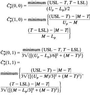
and C p m k , respectively:

(2)

MATHEMATICAL CORNER 387 minimum {

USL

-

T, T

-

LSL}

CE(0,O)

= (UP - L,)/2

(USL

-

T )

-

IM

-

q

C;(I,

0) = minimum 7

1

(T-LSL)-IM-T[1

M

- L, minimum {

USL

- T , T

-

LSL}

CE(0,l) = q(l,l) = 3 m u p - LP)/612 + ( M

-

T)’}

(T-LSL)-IM-

7l

3V{

[

(M - L,/3]’

+

(M

-

T)’}

3 . A

NEW

ESTIMATING METHOD In this section, we consider a new estimation method to obtain estimators of C and c p k for non-normal

Pearsonian populations. fnstead of estimating the two 3 a by

Up

-

M

and

M

- L,, respectively, we replace the two 3a by (Up - L,)/2. The new esti- mators of C, and c p k can be written as

-

USL-LSL

c,

=

UP

- LP

min{USL - M, M -

LSL}

dipk =

Applying the same method to the two more advanced (second and third generations) of PCIs, C,, and Cpmk, we obtain

USL

-

LSL

cpm = 6 d {

[(

Up

-

L,)/6]’

+

(M

-

T)’}

minimum{

USL

-

M , M

-

LSL}

Cpmk = 3 d {

[

( Up

-

L,)/6I2

+ (M

-

T)’}

The corresponding Vannman’s superstructure8 of these new estimators follows immediately:

d

-

ulM

-

ml

6V{

[

( Up - L,)/6]’

+

v

(M

- T)’}

Cp(u, v )

=

It is easy to verify that

In the case where the target is uncentred, Vannman’s superstructure can be easily generalized to the following:

min {

USL

-

T, T

-

LSL}

- ulM - 7l

3d{ [(

Up

- LP)/6]’

+

v

(M

-

T)’}

G(u,

v )

=

Consequently, by setting u =

0

and 1, v =

0

and 1, we obtain the following four estimators for the indices,

C,,

Cpk,

C,,

and C p m k , respectively:

q,

=

C(0,l)

- minimum {

USL

-

T, T

-

LSL}

- 3 d {

[

( Up - L,)/6]’

+

(M

-

T)’}

G m k = c:(1, 1) - minimum {

USL

-

T,

T

-

LSL}

-

IM

-

q

-

3V{

[ ( Up - L,)/6]’

+

(M - T)’}

LSL

Target USL 10 12 14 16 18 A 14-00 11.00 12.00 2.00 1-33 0-33 0.32 B 16.00 13.00 14.00 2.00 2-67 2-00 2-67 C 18.00 15.00 16@0 1 .00 1.33 0.32 0.32

(3)

388

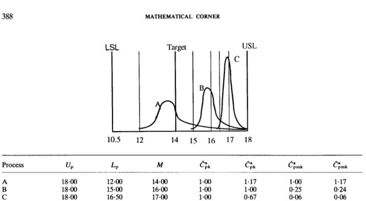
MATHEMATICAL CORNER

A 18.00 12.00 14.00 1.00 1.17 1.00 1.17

B 18.00 15.00 16-00 1.00 1.00 0.25 0.24

C 18.00 16-50 17-00 1 -00 0.67 0.06 0-06

Figure 2. An example of non-normal populations with an unentered target

4. COMPARISONS

To compare the new estimating method with Clem- ents’, we consider the examples depicted in Figure 1 and Figure 2. Figure 1 presents an example of three different non-normal populations with a centred target. The upper specification USL = 18, the lower specification LSL = 10. The target value

T

for this particular product is preset ot

14.

Figure 2 presents an example of three different non-normal populations with an uncentred target. The upper specification USL = 18, the lower specification

LSL

= 10.5. The target value

T

for this particular product is also preset to 14. The worksheet provided by Clements (Figure

3

of Reference 1) for calculating the estimators

of

the capability indices may be used to compute the values of those indices.

In Figure 1 we note that all three processes have same variabilities. Therefore, the quality of process B (which is on-target) is considered to be better than those of processes A and

C

(which are off- target). Clements’ estimator, t p k , in this case, shows

no sensitivity to the target at all ( t p k = 2.00 j o r processes A and B). But, the new estimator, Cpk,

clearly differentiates process

B

(which is on-target) from processes A and

C

(which are off-target).

In Figure

2,

the quality

of

process

A

is considered to be better than that of process

B.

Similarly, the quality of process B is considered to be better than that of process

C.

Clements’ estimator,

e

once again, shows no sensitivity to the target at aylin this particular case ( t p k =

1 . 0 ~

for all three processes).

But, the new estimator, Cpk, clearly differentiates

process A (which is on-target) from processes

B

and C (which are off-target).

5.

CONCLUSIONS

In this paper, we first investigated Clements’ method for calculating the estimators of the four capability indices, Cp, Cpk, Cp, and Cpmk for non-normal

populations. Then, we considered a new estimating method to calculate estimators of the four capability indices for non-normal Pearsonian populations. Both cases with centred and uncentred targets are investigated. Superstructures for those estimators

were also obtained for centred and uncentred cases. The analysis showed that the estimators calculated from the proposed new method can differentiate on-target processes from off-target processes better than those obtained by applying Clements’ method.

REFERENCES

1 . J. A. Clements, ‘Process capability calculations for non-nor- ma1 distributions’, Quality Progress, 22, 95-100 (1989). 2. W. L. Pearn and S. Kotz, ‘Application of Clements’ method

for calculating second and third generation process capability indices for non-normal Pearsonian populations’, to appear in

Quality Engineering.

3. L. K. Chan, S. W. Cheng and F. A . Spiring, ‘A new measure of process capability C,,’, Journal of Quality Technology, 20, 4. W. L. Pearn, S. Kotz and N. L. Johnson, ‘Distributional and inferential properties of process capability indices’, Journal of Quality Technology, 24, (4), 216-231 (1992).

5. V. E. Kane, ‘Process capability indices’, Journal of Quality Technology, 18, ( l ) , 41-52 (1986).

6. S. Kotz, W. L. Pearn and N. L. Johnson, ‘Some process

capability indices are more reliable than one might think’,

Journal of the Royal Statistical Society, Series C: Applied Statistics, 42, ( l ) , 55-62 (1993).

7. G . F. Gruska, K. Mirkhani and L. R. Lamberson, Non Nor- mal Data Analysis, Multiface Publishing Co., Michigan, 1989. 8. K. Vannman, ‘A unified approach to capability indices’, to

appear in Staristica Sinica.

(3), 162-175 (1988).

Authors’ biographies:

W. L. Pearn received his Ph.D. degree in Operations

Research from the University of Maryland at College

Park. He worked for AT&T Bell Laboratories Switch

Network Control and Process Quality Centers. Currently, Dr. Pearn is a professor of Operations Research at the Department of Industrial Engineering & Management,

National Chiao Tung University, Taiwan, Republic of

China.

K. S. Chen received his M.S. degree in Statistics from National Cheng Kung University. Currently, he is a Ph.D.

candidate at the Department of Industrial Engineering and Management, National Chiao Tung University.