Forecasting Time-Varying Covariance with a Robust Bayesian Threshold Model

(1)

Forecasting Time-Varying Covariance

with a Robust Bayesian Threshold Model

CHIH-CHIANG WU1

* AND JACK C. LEE2

1_{Department of Finance, Yuan Ze University, Taoyuan, Taiwan} 2

Graduate Institute of Finance, National Chiao Tung University, Hsinchu, Taiwan

ABSTRACT

This paper proposes a robust multivariate threshold vector autoregressive model with generalized autoregressive conditional heteroskedasticities and dynamic conditional correlations to describe conditional mean, volatility and correlation asymmetries in fi nancial markets. In addition, the threshold variable for regime switching is formulated as a weighted average of endogenous vari-ables to eliminate excessively subjective belief in the threshold variable deci-sion and to serve as the proxy in deciding which market should be the price leader. The estimation is performed using Markov chain Monte Carlo methods. Furthermore, several meaningful criteria are introduced to assess the forecast-ing performance in the conditional covariance matrix. The proposed methodol-ogy is illustrated using daily S&P500 futures and spot prices. Copyright © 2010 John Wiley & Sons, Ltd.

key words dynamic conditional correlation; generalized autoregressive con-ditional heteroskedasticity; hedge performance; Markov chain Monte Carlo; value at risk

INTRODUCTION

The vector autoregressive (VAR) model, popularized by Sims (1980), has been used widely and extensively by economists to study the dynamic behavior of economic variables. However, most covariance matrices of fi nancial asset returns are serially correlated, and multivariate generalized autoregressive conditional heteroskedastic (GARCH) models that have been introduced to take care of this problem have become increasingly popular in fi nancial econometrics in the past decade. A number of different multivariate GARCH models have been proposed, including the simplifi ed diagonal VECH model of Bollerslev et al. (1988), the BEKK model of Engle and Kroner (1995), the constant conditional correlation (CCC) model of Bollerslev (1990), the factor ARCH model of Engle et al. (1990) and the dynamic conditional correlation (DCC) model of Engle (2002). In par-ticular, the DCC-GARCH model is simpler and has successfully solved many practical problems. For example, hedges require estimates of the correlation between the returns on the assets. It is well Published online 25 May 2010 in Wiley Online Library

(wileyonlinelibrary.com) DOI: 10.1002/for.1183

* Correspondence to: Chih-Chiang Wu, Department of Finance, Yuan Ze University, 135 Yuan-Tung Road, Chungli, Taoyuan, Taiwan 320. E-mail: chihchiang@saturn.yzu.edu.tw

(2)

known that fi nancial market volatility changes over time. If the correlations and volatility are chang-ing, then the hedge ratio should be adjusted to account for the most recent information. In addition, the construction of an optimal portfolio with a set of constraints requires a forecast of the covariance matrix of returns.

Furthermore, multivariate threshold models are widely applicable, including co-integrated systems. A growing body of research in the recent time series literature has concentrated on incorporating nonlinear behavior in conventional linear reduced-form specifi cations such as autoregressive and moving average models. The motivation for moving away from the traditional linear model with constant parameters has typically come from the observation that many economic and fi nancial time series are often characterized by regime-specifi c behavior and asymmetric responses to shocks. For such series the linearity and parameter constancy restrictions are typically inappropriate and may lead to misleading inferences about their dynamics.

We next consider the situation in which each linear regime follows an autoregressive process. For instance, we have the well-known threshold autoregressive class of models, the statistical properties of which have been investigated in the early work of Tong (1990) and Tsay (1989). Multivariate threshold VARs are piecewise linear models with different autoregressive matrices in each regime, which is determined by a transition variable (one of the endogenous variables), a delay and a thresh-old (see Tsay, 1998). They were more recently reconsidered and extended in Hansen (2000) and Caner and Hansen (2001), among others. Hansen and Seo (2002) examined a two-regime vector error correction model with a single co-integrated vector and a threshold.

Bayesian methods have also recently become popular to researchers in econometrics. The VAR model usually has a large number of parameters, which are often estimated by means of maximum likelihood or least squares. In the threshold VAR, however, fi nite-sample frequentist analysis of the nonlinear functions is diffi cult. For instance, for some distributions of data, the maximum likelihood estimation (MLE) does not have an analytical form or simply does not exist, or in some applications of VAR models nonlinear functions of VAR parameters are the focus of research. The diffi culties faced in the frequentist approach to VAR inference can be circumvented by the Bayesian approach, which combines information from observations with researchers’ priors. When the objective of the model is to forecast, the Bayesian approach is more satisfactory. This approach consists of imposing prior restrictions on the VAR model parameters. The estimates of the model parameters are obtained by combining the prior belief and the likelihood, so that more accurate forecasts can be achieved (see Bauwens et al., 1999; Vrontos et al., 2003; Osiewalski and Pipien´, 2004; So et al., 2005).

In this paper, we present a robust threshold VAR (or VECM)-DCC-GARCH model and use the Metropolis–Hastings (MH) algorithm and the Gibbs sampling algorithm to estimate the parameters simultaneously. Our model extends existing approaches by admitting thresholds in conditional means, conditional volatilities and correlations of multivariate time series. Such an extension allows us to account for rich asymmetric effects and dependencies of conditional means, volatilities and correlations, as they are often encountered in practical fi nancial applications. In addition, we use the concept of Chen and So (2006) to defi ne the threshold variables as the linear combination of endog-enous variables. This setting can eliminate excessively subjective belief in threshold variable deci-sion. Besides, the weight coeffi cient can serve as the proxy in deciding which market is the price leader and which market is the price follower. Finally, the threshold values in our model are not fi xed ex ante but are estimated from the data, together with all other parameters in the model.

We investigate the empirical performance of our model in the S&P500 futures and spot markets. Our study attempts to use the posterior odds ratio and Bayes factors as a formal tool for making comparisons between competing models. We reduce our testing problem to a Bayesian model

(3)

selection problem. We can then select the model with a higher posterior odds ratio. We also present the performance comparison results of the one-step-ahead forecast in the conditional covariance matrix. The forecast results are assessed by several criteria which include the views of statistical loss and risk managers.

Based on the estimation results, we fi nd that the asymmetric dynamic structure is obvious in the dynamic relationship between the S&P500 futures and spot markets. We also detect that the S&P500 futures market is the price leader between the S&P500 futures and spot markets. Furthermore, based on several in-sample and out-of-sample performance measures in the conditional covariance matrix prediction, we fi nd that the threshold model outperforms the linear model across most measurement criteria.

The rest of the paper is organized as follows. In the next section, a robust multivariate threshold vector autoregressive is introduced. Then, the Bayesian approach is specifi ed including the setting of the priors, and then the conditional posterior distributions for relevant parameters are derived. In addition, the Markov chain Monte Carlo (MCMC) simulation method and implementation algorithm are taken into consideration. We then illustrate the empirical applications and the model performance comparisons. Finally brief conclusions are given.

1 , 0 ≤ wk ≤ 1, wk k K =

∑

= 1

1. Φ0(g) is the intercept vector, the Φl(g) for

l = 1, . . . , Lg are regression coeffi cient matrices in the gth regime, Lg∈ ⺞ is the lag of VAR in

the gth regime, εt is an innovation term, and d ∈ ⺞ is the threshold lag of the model with maximum delay d0. ᑣt-1 is the information set up to t − 1, and Ht is the time-varying

covariance matrix with elements hii,t and hij,t, i = 1, . . . , K, i = 1, . . . , K, j = i + 1, . . . , K. Rt is a

(4)

hii t i g , ⋅ω( )>0, αip (g) _{≥ 0, β} iq (g) _{≥ 0,} _α _β ip g p m iq g q n g g ( ) = ( ) =

∑

+

∑

< 1 1

1, 䊊 is the Hadamard matrix product operator, ηt= Dt−1εt is the vector of standardized errors, Q

−(g)

is the unconditional correlation matrix of εt in the gth regime, and the parameters A

(g)

and B(g)

are symmetric and positive semidefi nite matrices. To ensure that Q is positive semidefi nite, we also restrict (ıı′ − A(g)_{− B}(g)

) being positive semidefi nite. In addition, the threshold values rg must satisfy −∞ = r0< r1 < . . . < rG= ∞, and thus

the intervals [rg−1, rg), j = 1, . . . , G, form a partition of the space of zt−d.

The threshold variable zt−d is defi ned by a weighted average of yit−d and this can be viewed as a

extension of Tsay (1998) and Brooks (2001), who set the threshold variable to be a specifi c endog-enous variable,yit−d. We think that this setting of the threshold variable may have the following

advantages and economic meanings. First, when the yit−d are the returns of different markets, we can

regard wk and zt−d as the weight and the return of a portfolio without short sales, respectively, and

the dynamic structure or leverage effect may be infl uenced by the portfolio return. That is, the structural change in the markets may rely on the global economic conditions instead of a specifi c market condition. Second, the setting of the threshold variable can eliminate excessively subjective beliefs in the threshold variable decision and allow the data to choose a more appropriate zt−d by

estimating the weights, wk. Third, the weights wk can refl ect the relative signifi cance of each

endog-enous variable yit−d. This cannot only govern the time series behavior of Yt but from it we can also

fi nd which market is the price leader and which markets are price followers.

Under the assumption of conditional normality for the error process in equation (2), the likelihood function for the parameters can be expressed as

L K t t t t t P T K t t t y H H D R D q e e ( )= ( )

{

− ′

}

= ( ) − − − = + − −

∏

2 1 2 2 2 1 2 1 1 2 1 π π exp 2 2 1 1 1 2 exp

{

− ′( )−

}

= +

∏

et t t t et t P T D R D (7)

where θ is the set of all parameters, P = max(L1, . . . , LG, m1, . . . , mg, n1, . . . , ng, d0), and εt, Dt,

and Rt obey equations (1), (4), and (5), respectively.

However, when the variables Yt in the model are integrated and of order one or more, performing

the estimation by means of equation (1) is subject to the hazard of regressions involving nonstation-ary variables. In addition, Engle and Yoo (1987) have also argued that, in the presence of co-integration, a VAR model with an error correction mechanism should outperform a VAR over a longer forecasting horizon. Therefore, by taking into account the explicitly long-run equilibrium relationship, the mean equation (1) is modifi ed to the threshold vector error correction model, which can be written as DYt a b Yg t F F DY g l g t l l P g t d g g I r z r = ⎛ ′ + + ⎝⎜ ( ) − ( ) ( ) −⎞⎠⎟⋅

(

≤ < = − −

∑

1 0 1 1

))

⎡ ⎣⎢ ⎤ ⎦⎥+ =

∑

g G t 1 e (8)

where Δ denotes the difference operator, zt wk ykt k K = ⋅ =

∑

Δ 1

, b is the K × γ full rank matrix of co-integrating vectors, a(g)

(5)

correction terms, and the value γ determines the number of co-integrating relationships (γ < K). To Avoid the identifi cation problem, we impose the so-called linear normalization where b = (Iγ bo)′.

Thus the likelihood function for the parameters is similar to equation (7) except that εt must follow

equation (8).

BAYESIAN INFERENCE AND MCMC IMPLEMENTATION

In this section, we fi rst explain why the Bayesian method is used in this paper to analyze the threshold VAR (or VECM)-DCC-GARCH models. The reason is that by using the maximum likelihood method it is diffi cult to estimate the parameters in the threshold VAR-DCC-GARCH models. The main problems are the large number of parameters to be estimated and the diffi culty of estimation due to the positive defi niteness restrictions of the covariance matrix. This will therefore result in unstable estimates. In addition, due to the unknown threshold variable zt in this paper, we are

pre-vented from implementing a two-step estimation procedure similar to that considered by Tsay (1998) and Brooks (2001). Even if the threshold variable is known, Tsay (1998) showed that the asymptotic properties for the threshold lag, d, and the threshold parameter, rg, are hard to infer. Thus, to

deal with the above unfeasible procedure by using the maximum likelihood method, we extend the Bayesian method using MCMC techniques introduced by Chen and So (2006).

The implementation of the Bayesian analysis depends on a willingness to assign probability dis-tributions not only to the data variable y but also to all unknown parameters. Consider a situation in which absolutely weak previous subjective information is known about the phenomenon of interest, so as to mitigate frequentist criticisms of intentional subjectivity. In this paper, we choose non-informative or weakly non-informative priors for most parameters to interject the least amount of prior knowledge. The specifi cation of priors is listed below.

First, we assume that the discrete uniform prior for the threshold lag parameter d with maximum delay d0 can be written as π(d) = 1/d0, d = 1, . . . , d0, and does not favor any one of the candidate d values over any other. Since the weighted vector w = (w1, . . . , wK) relies on d, the conditional

prior of w given d, π(w|d) is assumed to be a symmetric Dirichlet distribution, w|d ~ D(δ, . . . , δ ), where the hyper-parameter δ > 0. Similarly, zt−d depends on d and w, and so we assume the condi-tional prior of every threshold parameter, rg, for g = 1, . . . , G − 1, to be a continuously bounded

uniform distribution, π(rg|d, w) = 1/(rup(g)− r(g)low), r(g)low ≤ rg≤ rup(g). The lower and upper bounds of the threshold parameters are employed to ensure that at least τ% of the observations are in each regime. In addition, τ depends on the number of observations. When the sample size is small, a higher τ is recommended. The purpose of this setting is to make the parameter estimates more effi cient and more reliable.

We subsequently divide the parameters in each regime into four independent blocks, which are the parameters in the VAR model (1, 8), the error correction term (8), the volatility process (4), and the dynamic correlation procedure (6), and we assume that the priors are independent between any two regimes. For the priors of the VAR parameters, Litterman (1980) and Kinal and Ratner (1986) have indicated that VAR sometimes suffers from overparameterization. The requirement that a large number of coeffi cients in VAR be estimated often leads to large standard errors for inferences and forecasts. The imposition by the Bayesian VAR of some prior restrictions on parameters will usually provide more accurate forecasts. In this paper, we adopt Litterman’s (1980) Minnesota prior for VAR parameters and make some appropriate modifi cations. For convenience, we defi ne Φ(g)_{= [Φ}

0 (g)

,

(6)

we denote by φ(g)

. We assume that the vector φ(g)

follows a multivariate normal distribution with zero mean and diagonal covariance matrix Σφ. That is, we believe in advance that the unconditional mean

and short-run dynamics center around zero, and that investors are unable to earn excess returns based on this short-run dynamic relationship. In addition, the priors are made independently across ele-ments of φ(g)

, and the standard deviation of the coeffi cient φijl

(g)

, which is an element of φ(g) and describes how variable i is affected by variable j of lag l in the gth regime, is given by

S φ λ η λ τ τ ijl g i j l i j l i j ( )

( )

= = ⋅ ≠ ⎧ ⎨ ⎪⎪ ⎩ ⎪ ⎪ if if (9)

where the hyper-parameter λ controls the tightness of beliefs on φ(g)

, τi/τj is a correction for the scale

of series i compared with series j, and the restriction 0 < η < 1 implies that the series are more likely to be infl uenced by their own lags than by the lags of other series.

The above model requires that we choose specifi c values for the hyper-parameters λ, τi, τj, and

η. The correction term τi/τjis used in modifying the inconsistency in variation of each series variable.

While in principle these should be chosen on the basis of a priori reasoning or knowledge, we will in practice follow Litterman (1986) in choosing these as the sample standard deviations of residuals from univariate autoregressive models that fi t the individual series in the sample. For the remaining hyper-parameters, λ is commonly set from 0.1 to 0.9, and η ranges from 0.2 to 0.5 (see Litterman, 1986; Doan, 1990). In addition, Villani (2001) showed that the selection of these two parameters is not sensitive to the forecasting results. We therefore use λ = 0.5 and η = 0.4 in our empirical analysis. We also set the standard deviation of the intercept coeffi cient to 1 to employ a more diffuse prior.

For the prior on the long-term structure (i.e., the error correction term) in each regime, we follow Geweke (1996) to choose uniform priors for both the matrix of co-integrating vectors b(g)

and the associated weighting matrix a(g)

, and the prior can be written as π(a(g) , b(g)

) ∝ 1. Furthermore, a uniform prior with some restrictions is assumed for the parameters of the GARCH and is written as

π w ag g b g ω α β α i g ip g iq g ip g p m I g ( ) ( ) ( ) ( ) ( ) ( ) ( ) =

(

, ,

)

∝ >0; ≥0; ≥0;

∑

+ 1 ββiq g q n i K g ( ) = =

∑

∏

⎛ < ⎝⎜ ⎞ ⎠⎟ 1 1 1 (10)

where I(·) is the indicator function, which takes on a value of unity if the constraint holds and zero otherwise, and ω(g)= (ω1 (g) , . . . , ωK (g) ), α(g)= (αi1 (g) , . . . , α(g)img, αK1 (g) , . . . , α(g)Kmg), and β (g) = (βi1 (g) , . . . , β(g) img, . . . , βK1 (g)

, . . . , β(g)Kmg). Finally, we also choose a uniform prior for the dynamic correlation

structure

π A B Qg g g I ( ) ( ) ( )

(

, ,

)

∝ ( ) (11)

where ϒ is the set of (A(g) , B(g),

Q−(g)), which must satisfy the requirement that A(g) , B(g)

, and (ıı′ − A(g) − B(g)

)are symmetric and positive semidefi nite matrices, and Q−(g)is a form of the correlation coeffi -cient matrix. Therefore, the prior of all unknown parameters in the threshold VAR-DCC-GARCH model can be expressed as

(7)

π π π π π π q f w a b ( )∝ ( ) ( )⎛_⎝⎜

(

)

⎞_⎠⎟ ⋅

( )

= − ( ) ( ) ( ) ( )

∏

d d r dg g G g g g g w ,w , , 1 1

((

)

(

)

⎛ ⎝⎜ ⎞ ⎠⎟ ( ) ( ) ( ) =

∏

π A B Qg g g g G , , 1 (12)

Bayesian inference regarding the parameter vector θ conditional upon the data matrix y is con-structed through the posterior density p(θ|y). Using Bayes’ theorem, the posterior density is formed by the prior density π(θ) and the likelihood L(y|θ), and it can be expressed as

p L L L q q q q q q q q y y y y ( )= ( ) ( ) ( ) ( ) ∝ ( ) ( )

∫

π π d π (13)

Therefore, the optimal Bayes estimator of θ under quadratic loss is simply the posterior mean, which is

ˆ

q=E(qY)=

_∫

q qp( y)dq (14)

However, for many realistic problems, the posterior distribution p(θ|y) may not have an analyti-cally tractable form, particularly for high dimensions, and so calculating the posterior mean is a diffi cult task. In fact, to settle our major problems, we can use numerical or asymptotic methods to compute the approximate posterior mean for the full Bayesian model. Because the posterior density has a very high dimension and is only known up to a constant, in this paper we adopt the MCMC sample algorithm as our tool for this purpose.

We will therefore subsequently use Bayes factors to select the appropriate order of the VAR process and to choose between linear (G = 1) and nonlinear (G ≥ 2) versions of our model. When comparing any two competing parametric Bayesian models (Mi, Mj) for the same data matrix y, the

Bayes factor (BF) can be calculated based on the marginal likelihood concept. In general terms, by letting θj be the appropriate set of parameters under model Mj, the marginal likelihood can be

written as p Mj p Mj p Mj j j y y

(

)

=

_∫

(

q,

) (

q

)

dq Θ (15)

where p(y|θ, Mj) and p(θ|Mj) are the sampling density function and the prior density function,

respectively.

For the Bayesian model selection, we can determine the posterior odds ratio (POR) of Mi against

Mj by the Bayes factors Bij = p(y|Mi)/p(y|Mj) and the prior odds ratio p(Mi)/p(Mj), and it can be

expressed as PORij i j i j ij p M p M p M p M B =

₍

( y_y)

₎

=

_{( )}

( ) (16)

If there is an absence of a prior preference for either model, i.e., p(Mi) = p(Mj) = 1/2, the Bayes

(8)

> 1 the data prefer Mi over Mj, and when Bij< 1 the data favor Mj over Mi. Thus, in this paper, we

can compare any two threshold VAR-GARCH time series models of different orders and regimes by computing Bayes factors as the ratio of the marginal likelihood concept evaluated along the route of Chib (1995).

EMPIRICAL APPLICATIONS

Data description

The models are applied to daily data on the S&P500 index and S&P500 index futures for the period 3 January 1995 to 31 October 2007. The sample size for each stock market is 3221. Both spot and futures prices are collected from TICK DATA. For S&P500 index futures, we switch to a new contract as the contract’s maturity approaches in order to construct a continuous futures contract series. To avoid thin markets and expiration effects, we roll over to the next nearest contract at least one week prior to the expiration of the current contract. The daily spot and futures returns are calculated as the differences in the logarithms of daily price indices multiplied by 100. In addition, intraday 5-minute prices are used to construct the series of realized covariances, as was the case in similar related studies in the past.

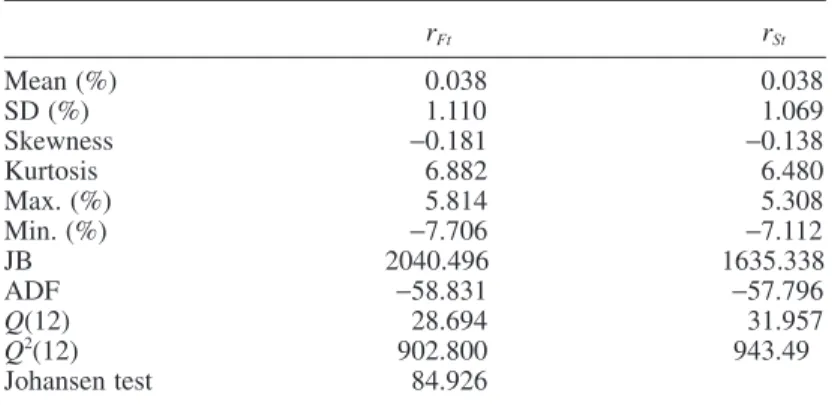
The descriptive statistics for S&P500 spot and futures returns are summarized in Table I. The statistics reported are the sample mean, standard deviation, maximum, minimum, Jarque–Bera (JB) statistics, and the Ljung–Box (LB) statistics for the return and the square return series. The standard deviation of futures returns is larger than that of the spot returns, indicating that the futures market is more volatile than the spot market. Both spot and futures returns are negatively skewed and present concerns for excess kurtosis. The JB test statistics provide clear evidence that reject the null

Table I. Descriptive statistics for S&P500 futures and spot returns

rFt rSt Mean (%) 0.038 0.038 SD (%) 1.110 1.069 Skewness −0.181 −0.138 Kurtosis 6.882 6.480 Max. (%) 5.814 5.308 Min. (%) −7.706 −7.112 JB 2040.496 1635.338 ADF −58.831 −57.796 Q(12) 28.694 31.957 Q2₍₁₂₎ _902.800 _943.49 Johansen test 84.926

Note: This table reports the descriptive statistics for daily S&P500 futures and spot returns for the sample period from 3 January 1995 to 31 October 2007. rFt and rSt

refer to S&P500 futures and spot returns, respectively. Daily returns are calculated by 100 × (ln(Pt) − ln(Pt−1)). The values in rows JB, ADF and Johansen are statistics

of the Jarque–Bera normality test, the augmented Dickey–Fuller unit root test, and the Johansen co-integration test, respectively. Q(12) and Q2_{(12) report the Ljung–}

Box (LB) portmanteau test statistics including 12 lags for the return and square return series. The critical values at the 5% level of the JB, ADF, Johansen, and LB statistics are 5.991, −2.862, 15.495, and 21.026, respectively.

(9)

hypothesis of normality for each returns series and this is mainly due to the presence of skewness and excess kurtosis. The augmented Dickey–Fuller unit root test results suggest that both return series are stationary. The LB Q statistics indicate possible serial correlations for both returns series. Moreover, the Q2

statistics suggest that there are autoregressive conditional heteroskedasticity effects on each returns series. The Johansen co-integration test indicates a long-run equilibrium relationship between S&P500 spot and futures indices.

Goodness-of-fi t results

In this section, we apply the bivariate threshold VECM-DCC-GARCH model to the S&P500 futures and spot markets. We also use two different time lengths (5 years and 10 years) to perform model comparisons. In addition, we simplify our model by assuming that L1 = . . . = LG = L, and the

GARCH(1,1) model is considered to be a parsimonious model that is found to be appropriate in most applications. The matrix parameters A(g)

and B(g)

in equation (6) are also reduced to scale parameters. Thus, to ensure that Q is positive semidefi nite, we restrict A(g)_{+ B}(g)_{< 1, for g = 1, . . . ,} G. Therefore, we only need to choose proper L and G based on the Bayes factor criterion.

To implement our MCMC sampling scheme, we carry out 30,000 iterations, which are performed with the fi rst 10,000 burn-in iterations discarded, to reach the convergence of every parameter. The logarithmic marginal likelihood, the logarithmic Bayes factors, which are on the basis of a simple linear VECM(1)-DCC-GARCH(1, 1) model, and the overall ranking of models for different L and G, are shown in Table II. For the period 2000–2004, Table II shows that the best model to describe the dynamic relationship between the S&P500 futures and spot markets is the two-regime threshold VECM(3)-DCC-GARCH(1, 1) model with a logarithm of the marginal likelihood value of −1926.714. If we compare the best model with the linear VECM(1)-DCC-GARCH(1, 1) model, i.e., a model in which there is no asymmetric effect on the mean, variance, and correlation equations, then the dif-ference in the logarithmic marginal likelihood is ln(B6,1) = 69.606, which yields a Bayes factor of B6,1 = 1.696 × 1030

. This means the two-regime threshold VECM(3)-DCC-GARCH(1, 1) model is 1.696 × 1030

times more likely than the linear VECM(1)-DCC-GARCH(1, 1) model. Table II also indicates that the two-regime threshold VECM(3)-DCC-GARCH(1, 1) model is more satisfactory than the other competitors considered here, regardless of whether 5-year or 10-year data are used. Generally speaking, the results in Table II show that models which consider asymmetric effects and longer lags have larger logarithms of marginal likelihood. This suggests that there are asymmetric effects on the mean, covariance, or error correction processes in regard to the dynamic relationship between the S&P500 futures and spot markets. In addition, the logarithmic marginal likelihood of the model with longer lags is larger than that with shorter lags, suggesting that taking longer lags into consideration will benefi t the model’s explanatory power.

Bayesian estimation results

In this section, we will illustrate the Bayesian estimation results for the period 1995–2004. The linear and threshold VECM(3)-DCC-GARCH(1, 1) models estimation results for the mean equation (8) and variance–covariance matrix equations (4–6) for the dynamic relationship between S&P500 futures and spot markets are presented in Table III. In the three-regime threshold model, the feedback effects between each pair of S&P500 futures and spot markets are observed for all kinds of market conditions (i.e., downside, neutral, and upside markets). That is, lagged spot (futures) returns help to predict current futures (spot) returns. In addition, most lagged spot (futures) returns have negative effects on current spot (futures) returns except for the futures returns in the upside market. The futures (spot) returns tend to decrease (increase) when the spread is large in order to restore the

(10)

T

able II.

Logarithms of mar

ginal likelihood and Bayes factors for S&P500 futures and spot markets

Model ( Mi ) Number of parameters 2000–2004 (5 years) 1995–2004 (10 years) ln[ p (y |Mi )] ln( Bi,1 ) Rank ln[ p (y |Mi )] ln( Bi,1 ) Rank M1 , VECM(1)-DCC-GARCH(1, 1) 18 − 1996.319 0 9 − 3724.953 0 9 M2 , VECM(2)-DCC-GARCH(1, 1) 22 − 1956.541 39.778 5 − 3663.752 61.201 6 M3 , VECM(3)-DCC-GARCH(1, 1) 26 − 1948.295 48.025 4 − 3633.945 91.007 4 M4 , 2R-VECM(1)-DCC-GARCH(1, 1) 38 − 1960.836 35.483 6 − 3680.614 44.338 7 M5 , 2R-VECM(2)-DCC-GARCH(1, 1) 46 − 1941.648 54.671 2 − 3614.597 1 10.355 2 M6 , 2R-VECM(3)-DCC-GARCH(1, 1) 54 − 1926.714 69.606 1 − 3589.465 135.488 1 M7 , 3R-VECM(1)-DCC-GARCH(1, 1) 56 − 1990.747 5.573 8 − 3710.036 14.916 8 M8 , 3R-VECM(2)-DCC-GARCH(1, 1) 68 − 1976.574 19.745 7 − 3649.549 75.404 5 M9 , 3R-VECM(3)-DCC-GARCH(1, 1) 80 − 1942.786 53.534 3 − 3627.081 97.871 3 Note :

The table shows the number of parameters, logarithms of mar

ginal likelihood, logarithms of Bayes factors, and the ranks of ma

rginal likelihood for several

models and two dif

ferent time lengths.

The data are based on the daily S&P500 futures and spot market prices for the sample per

iod from 3 January 1995 to 31

(11)

T

able III.

Bayesian estimation results for the S&P500 futures and spot markets One regime

T wo regimes Three regimes zt−1 ≤ r1 zt−1 > r1 zt−1 ≤ r1 r1 < zt− 1 ≤ r2 zt−1 > r2 Δ ln Ft Δ ln St Δ ln Ft Δ ln St Δ ln Ft Δ ln St Δ ln Ft Δ ln St Δ ln Ft Δ ln St Δ ln Ft Δ ln St Mean equations φ.0 0.031 0.109 − 0.209 − 0.175 0.008 0.088 − 0.237 − 0.175 − 0.025 0.103 0.529 0.629 (0.033) (0.030)** (0.097)* (0.106) (0.030) (0.043) (0.161) (0.147) (0.027) (0.043)** (0.162)** (0.155)** φ .F1 − 0.222 0.388 − 0.201 0.442 − 0.354 0.234 − 0.194 0.475 − 0.368 0.243 − 0.025 0.493 (0.045)** (0.041)** (0.069)** (0.062)** (0.049)** (0.053)** (0.084)* (0.084)** (0.090)** (0.083)** (0.077) (0.060)** φ .F2 − 0.128 0.199 − 0.105 0.219 − 0.159 0.196 0.064 0.383 − 0.1 1 1 0.244 − 0.379 0.012 (0.026)** (0.025)** (0.107) (0.102)* (0.048)** (0.043)** (0.058) (0.052)** (0.056)* (0.054)** (0.071)** (0.067) φ .F3 − 0.158 0.015 − 0.074 0.1 10 − 0.129 0.048 0.309 0.479 − 0.136 0.050 − 0.646 − 0.431 (0.043)** (0.039) (0.129) (0.1 1 1 ) (0.044)** (0.034) (0.1 12)** (0.101)** (0.047)** (0.050) (0.147)** (0.146)** φ .S1 0.247 − 0.358 0.049 − 0.591 0.404 − 0.197 0.031 − 0.633 0.407 − 0.210 − 0.193 − 0.756 (0.050)** (0.047)** (0.043) (0.047)** (0.048)** (0.053)** (0.079) (0.080)** (0.070)** (0.067)** (0.058)** (0.056)** φ .S2 0.131 − 0.187 0.044 − 0.261 0.150 − 0.201 − 0.155 − 0.455 0.123 − 0.228 0.324 − 0.063 (0.033)** (0.033)** (0.098) (0.098)** (0.049)** (0.042)** (0.068)* (0.062)** (0.061)* (0.061)** (0.080)** (0.075) φ .S3 0.130 − 0.038 0.006 − 0.166 0.134 − 0.046 − 0.393 − 0.549 0.168 − 0.025 0.664 0.452 (0.043)** (0.038) (0.133) (0.1 16)* (0.046)** (0.038) (0.1 18)** (0.108)** (0.048)** (0.050) (0.174)** (0.175)** a − 0.821 0.838 − 0.451 0.376 − 0.786 0.818 − 0.478 0.402 − 0.690 0.816 − 0.293 0.268 (0.151)** (0.127)** (0.428) (0.472) (0.173)** (0.155)** (0.351) (0.503) (0.264)** (0.138)** (0.490) (0.435) b − 1.007 − 1.006 − 1.01 1 (0.005)** (0.006)** (0.005)** Thr eshold parameters d 1 # 1 # 1 # w1 0.671 0.758 (0.180)** (0.076)** r1 − 0.601 − 0.620 (0.033)** (0.022)** r2 1.301 (0.019)** V ariance–covariance equations ω 0.033 0.029 0.342 0.312 0.034 0.025 0.332 0.297 0.044 0.030 0.193 0.183 (0.005)** (0.005)** (0.038)** (0.035)** (0.005)** (0.004)** (0.037)** (0.034)** (0.006)** (0.005)** (0.088)* (0.079)** α 0.075 0.085 0.069 0.080 0.056 0.064 0.075 0.090 0.020 0.044 0.044 0.048 (0.007)** (0.009)** (0.010)** (0.013)** (0.01 1)** (0.012)** (0.013)** (0.015)** (0.013) (0.015)** (0.017)** (0.016)** β 0.899 0.890 0.855 0.836 0.852 0.853 0.851 0.827 0.846 0.847 0.834 0.832 (0.010)** (0.012)** (0.025)** (0.029)** (0.010)** (0.01 1)** (0.023)** (0.025)** (0.01 1)** (0.010)** (0.052)** (0.056)** A 0.137 0.139 0.232 0.155 0.265 0.165 (0.016)** (0.039)** (0.026)** (0.040)** (0.034)** (0.059)** B 0.083 0.122 0.1 14 0.136 0.066 0.582 (0.056) (0.089) (0.060) (0.099) (0.047) (0.178)** ρ− 0.975 0.972 0.976 0.972 0.976 0.910 (0.001)** (0.003)** (0.001)** (0.004)** (0.001)** (0.202)** Note :

This table shows the parameter estimates for one, two and three regime threshold

VECM(3)-DCC-GARCH(1,1) models, respectively

, which are based on the daily S&P500 futures

and spot market returns for the sample period from 3 January 1995 to 31 December 2004. Numbers in parentheses are standard devi

ations.

Asterisks indicate statistical signifi

cance at the

*

5% and **

1% levels.

# Posterior mode of the threshold lag parameter

(12)

long-run equilibrium relationship only in the neutral market. The evidence suggests that the S&P500 futures (spot) price tends to converge to the spot (futures) price and the effect is more apparent in the neutral market. Furthermore, the structures of the error correction terms are asymmetric for dif-ferent market conditions.

The weighted coeffi cient in the threshold variable, w1, is signifi cantly larger than 0.5, especially in the three-regime threshold model. This indicates that the S&P500 futures market is the price leader whereas the spot market is the price follower. Furthermore, we fi nd that the threshold values, r1 and r2, are not symmetric and point out the asymmetric dynamic structures between downside and upside markets. For the coeffi cients of the variance covariance equations, we fi nd that the volatility is most persistent in the downside market for both the futures and spot markets. However, the persistence of the correlation between futures and spot returns has an opposite outcome. In addition, the uncon-ditional correlation coeffi cients, ρ−, in the downside market is larger than that in the upside market. The short-term effects of shocks on the correlation are apparent in all kinds of market conditions, while the long-term correlation only infl uences the current correlation in the upside market.

Covariance matrix forecast comparison

In this section, the data from 3 January 2000 to 31 December 2004, consisting of 1256 trading days, are used for in-sample estimation and forecasting performance evaluation in the one-step-ahead conditional covariance matrix. The 702 observations from 3 January 2005 to 31 October 2007 are used for out-of-sample performance evaluation purposes. The out-of-sample forecasting procedure is carried out as follows. The models are estimated 702 times based on 702 samples of 1256 obser-vations. The fi rst sample, starting 3 January 2000 and ending 31 December 2004, is used to forecast the covariance matrix of 3 January 2005 based on the estimated model for the fi rst sample. The forecast of the covariance matrix is generated for 4 January 2005 based on the estimated model for the second sample, starting 4 January 2000 and ending 3 January 2005.These estimation and fore-casting steps can be repeated 702 times for the available sample and we produce the 702 one-step-ahead covariance matrix forecasts.

In addition, we present two categories of criteria to measure the forecasting performance of dif-ferent competitive models. One category is based on the views of the statistical loss function, which is a non-negative function that generally increases as the distance between the actual value and the forecast value increases, and three different types of criteria are adopted here. The other category of performance measure is based on the views of risk managers and two types of criteria are introduced.

Statistical loss performance

denote the forecast and realized values at time t, respectively.

The fi rst two loss functions are symmetric, which are the mean absolute error (MAE) statistic and the mean square error (MSE) statistic, respectively. The third loss function is asymmetric, which is the linear-exponential (LINEX) loss. When ζ is close to 0, the LINEX loss function is nearly sym-metric and is not much different from the MSE statistic. In the LINEX loss function, positive errors are weighed differently from the negative errors when ζ ≠ 0. If ζ > 0 (ζ < 0), the LINEX loss func-tion is approximately linear (exponential) for FCMt− RCMt< 0 and exponential (linear) for FCMt

− RCMt> 0. This implies that an overestimate (underestimate) needs to be taken more seriously into

consideration. More specifi cally, in all the above cases, a lower loss measure indicates a higher forecasting power.

As a result of the unobservable property of the covariance matrices, here we use intraday 5-minute data to construct the proxies for the daily-realized covariance observations. The concept of the real-ized volatility has been proposed by French et al. (1987) and Andersen et al. (2001). The realreal-ized volatility is nothing more than the sum of the squared high-frequency returns over a given sampling period. Similarly, we can directly express the realized covariance (RCOV) as

RCOV t R t j R t j j ,Δ Δ Δ, Δ Δ, Δ ( )= ( − + ⋅ ) ( − + ⋅ )′ =

∑

1 1 1 1 (20)

where R(t, Δ) denotes the K × 1 vector of logarithm returns over the [t − Δ, t] time interval. A comparison of the results of the forecast performance measures in the conditional covariance matrix between S&P500 futures and spot returns for the different models is presented in Table IV. When looking at the in-sample prediction, we observe that the threshold model yields better perfor-mance relative to the linear model for the forecast of covariance between the S&P500 futures and spot returns, cov(rFt, rSt), regardless of which symmetric (MAE and MSE) or asymmetric (LINEX)

loss functions are used. The better covariance forecast mainly comes from the improvement in the volatility forecast of the S&P500 futures and spot returns, var(rFt) and var(rSt). The results of the

correlation forecasts between S&P500 futures and spot returns, corr(rFt, rSt), for linear or threshold

models are similar. For the out-of-sample forecast, two-regime threshold models perform more appropriately for the covariance forecast, while three-regime threshold models have worse forecast-ing ability than linear models except for the VECM(3)-DCC-GARCH(1, 1) model.

Risk management performance

Predictability in the covariance between two assets’ returns, as measured by traditional criteria that focus on the size of the forecast error, does not necessarily imply that an investor can make profi ts or reduce risk from a trading strategy based on such forecasts. Therefore, we also use the other category of performance measure which is based on the views of risk managers, and two types of

(14)

T

able IV

.

In- and out-of-sample covariance matrix forecast comparison of alternative models for theS&P500 futures and spot mark

ets Model (M i ) var( rFt ) var( rSt ) In-sample Out-of-sample In-sample Out-of-sample MAE MSE LIN(1) LIN( − 1) MAE MSE LIN(1) LIN( − 1) MAE MSE LIN(1) LIN( − 1) MAE MSE LIN(1) LIN( − 1) M1 0.570 1.403 0.388 1909.047 0.237 0.127 0.050 0.158 0.478 0.874 0.258 57.141 0.234 0.1 18 0.047 0.1 15 M2 0.575 1.423 0.375 1770.966 0.224 0.122 0.047 0.156 0.481 0.888 0.252 53.131 0.226 0.1 13 0.045 0.1 10 M3 0.578 1.433 0.373 1774.181 0.214 0.1 17 0.045 0.147 0.483 0.895 0.252 53.038 0.219 0.1 1 1 0.043 0.108 M4 0.528 1.222 0.359 2013.272 0.218 0.1 13 0.050 0.094 0.436 0.753 0.237 52.151 0.180 0.090 0.037 0.075 M5 0.532 1.214 0.370 2198.489 0.223 0.1 16 0.050 0.099 0.438 0.744 0.243 53.517 0.183 0.093 0.039 0.076 M6 0.532 1.223 0.390 2130.491 0.21 1 0.104 0.044 0.085 0.438 0.748 0.248 51.837 0.175 0.084 0.035 0.066 M7 0.570 1.232 0.331 1819.310 0.293 0.152 0.066 0.123 0.456 0.737 0.220 48.226 0.231 0.1 12 0.047 0.087 M8 0.561 1.219 0.338 1931.171 0.268 0.140 0.059 0.1 19 0.450 0.735 0.226 49.383 0.209 0.105 0.043 0.084 M9 0.549 1.213 0.348 2152.719 0.203 0.108 0.046 0.095 0.446 0.730 0.230 51.930 0.168 0.087 0.035 0.074 Model (M i ) corr( rFt ,rSt ) cov( rFt ,rSt ) In-sample Out-of-sample In-sample Out-of-sample MAE MSE LIN(1) LIN( − 1) MAE MSE LIN(1) LIN( − 1) MAE MSE LIN(1) LIN( − 1) MAE MSE LIN(1) LIN( − 1) M1 0.045 0.004 0.002 0.002 0.054 0.004 0.002 0.002 0.451 0.736 0.237 16.692 0.208 0.104 0.040 0.1 17 M2 0.044 0.004 0.002 0.002 0.053 0.004 0.002 0.002 0.454 0.748 0.230 18.597 0.200 0.101 0.038 0.1 13 M3 0.045 0.004 0.002 0.002 0.055 0.004 0.002 0.002 0.456 0.753 0.230 18.698 0.191 0.098 0.036 0.109 M4 0.045 0.004 0.002 0.002 0.053 0.004 0.002 0.002 0.417 0.625 0.219 10.042 0.176 0.085 0.034 0.075 M5 0.045 0.004 0.002 0.002 0.054 0.004 0.002 0.002 0.419 0.619 0.224 10.341 0.180 0.088 0.035 0.077 M6 0.045 0.004 0.002 0.002 0.055 0.004 0.002 0.002 0.420 0.627 0.231 9.676 0.171 0.079 0.032 0.067 M7 0.045 0.004 0.002 0.002 0.054 0.004 0.002 0.002 0.441 0.623 0.204 9.670 0.235 0.1 10 0.045 0.090 M8 0.045 0.004 0.002 0.002 0.055 0.004 0.002 0.002 0.434 0.619 0.208 9.558 0.215 0.103 0.041 0.088 M9 0.045 0.004 0.002 0.002 0.055 0.004 0.002 0.002 0.428 0.612 0.212 9.212 0.166 0.083 0.032 0.075

(15)

criteria are used. One involves calculating the value at risk (VaR) as an evaluation of the estimator. For a two-asset portfolio with δ1 invested in the fi rst asset and δ2 in the second asset, the one-step-ahead VaR at time t and at α%, assuming normality, is

VaRt( )α = − (δ1 1rt+δ2 2r t)− ⋅zα δ1h t+δ h t+ δ δ h 2 11 2 2 22 2 1 2 1 ˆ, ˆ, ˆ , ˆ , ˆ22,t ⎡ ⎣ ⎤⎦ (21)

where za is the right quantile at α%. To compare and evaluate model performances for several

different model specifi cations, we choose the following criteria. By defi nition, the failure rate (FR) is the proportion of returns (in absolute value terms) that exceed the forecast VaR, i.e.

FR=( ) ( + < −VaR ( )) =

∑

1T _t₁I 1 1rt 2 2r t t T

δ , δ , α , where I(·) is the indicator function. Hence, if the VaR

model is correctly specifi ed, the failure rate should be equal to the prespecifi ed VaR level. We also use the Kupiec (1995) LR test to examine whether the model is correctly specifi ed. To test H0 : f = α against H1 : f ≠ α, the LR statistic is LR = −2 ln(αN

(1 − α)T−N₎_{+ 2 ln((N/T)}N

(1 − (N/T))T−N_{), where} N is the number of VaR violations, T is the total number of observations and f is the theoretical failure rate. Under the null hypothesis, the LR test statistic is asymptotically distributed as χ2

(1).

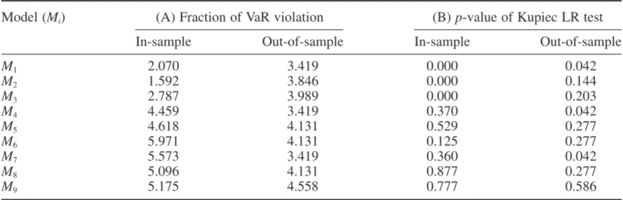
The fractions of VaR violations and p-values of the Kupiec (1995) failure rate test for a hedged portfolio with weights (δFutures, δspot) = (−1, 1) are reported in Table V. For in-sample data, the p-values for the null hypothesis of the hedged portfolio are all smaller than 0.05 when the linear model is considered. The threshold model performs very well as there are no p-values smaller than 0.05. Thus the switch from the linear model to the threshold model yields a signifi cant improvement in the VaR performance in the hedged portfolio. For the out-of-sample VaR performance comparison, the p-values of the linear and threshold models with the lag of VAR L = 1 are all smaller than 0.05. However, for L = 2 and L = 3, we fi nd that the fractions of the VaR violation based on the threshold model are closer to the prespecifi ed VaR level than those based on the linear model. In view of the in-sample and out-of-sample empirical results, we fi nd that the linear model may sometimes over-estimate the VaR, and so using the threshold model to calculate the portfolio’s VaR may be more appropriate.

Table V. In- and out-of-sample 5% VaR failure rate results for the S&P500 futures–spot hedged portfolio

Model (Mi) (A) Fraction of VaR violation (B) p-value of Kupiec LR test

In-sample Out-of-sample In-sample Out-of-sample

M1 2.070 3.419 0.000 0.042 M2 1.592 3.846 0.000 0.144 M3 2.787 3.989 0.000 0.203 M4 4.459 3.419 0.370 0.042 M5 4.618 4.131 0.529 0.277 M6 5.971 4.131 0.125 0.277 M7 5.573 3.419 0.360 0.042 M8 5.096 4.131 0.877 0.277 M9 5.175 4.558 0.777 0.586

Note: This table shows the 5% VaR forecast results of S&P500 futures–spot hedge portfolios for alternative models. Panel (A) is the fraction of VaR violations, and the results of the Kupiec LM test (1995) are shown in panel (B). The in-sample data period extends from 3 January 2000 to 31 December 2004 and the out-of-sample data period extends from 3 January 2005 to 31 October 2007. M1, M2, . . . , M9 refer to the same models as in Table II.

(16)

While futures contracts are popular among investors as a class of speculative assets, they are important in the fi nancial markets due to their use as a hedging instrument. Furthermore, hedging with futures contracts may be the simplest method to manage market risk resulting from adverse movements in the prices of various assets. In this section, we assume the hedger attempts to minimize the conditional variance of the spot–futures portfolio. It is well known that the optimal hedge ratio (OHR) is the ratio of the conditional covariance between spot and futures returns over the conditional variance of the futures return. Thus the one-step-ahead forecasts of optimal hedge ratios can then be calculated as

HR*t =covt+1t(r rs, f) vart+1t( )rf (22) where rs and rf are spot and futures returns, respectively. The variance of the estimated optimal hedged portfolio can be characterized as

var(rs,t−HR*t ⋅rf,t) (23)

To evaluate hedging performance, the typical criterion is based on the percentage variance reduc-tion (PVR) of the hedged portfolio relative to the unhedged posireduc-tion. It can be calculated as

PVR var hedged portfolio

var unhedged portfolio % ( )= − ( ) ( ) ⎛ ⎝⎜ ⎞⎠ 1 _⎟⎟ ⎡ ⎣⎢ ⎤ ⎦⎥×100% (24)

When the futures contract completely eliminates risk, PVR = 100 is obtained, otherwise PVR = 0 is obtained when hedging with the futures contract does not reduce risk. Hence a larger PVR indicates better hedging performance.

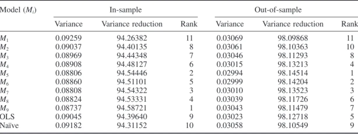
The in- and out-of-sample hedged portfolio variances and hedging effectiveness of alternative models for the S&P500 futures contract are presented in Table VI. The variances of hedged portfolio returns are calculated under the following 11 alternative models: three linear VECM-DCC-GARCH models with different lag parameters L(M1, M2, M3), six threshold VECM-DCC-GARCH models with different lag parameters L and the number of regimes G(M4, . . . , M9), hedging with a constant OHRs estimate using regression methods of returns and the naïve hedge with a hedge ratio of 1 at all times. The results show that the three-regime threshold VECM(3)-DCC-GARCH model has the lowest in-sample hedged portfolio variance, with a 94.587% in-sample variance reduction compared to the variance of the unhedged position. In addition, the in-sample hedging performance of the linear model with L = 1 is even worse than that of OLS or a naïve strategy.

However, active hedgers are likely to be more concerned about future hedging performance. Therefore, the comparison of out-of-sample performance is a better way to evaluate our hedging strategy. We fi nd that the ranking of out-of-sample hedging effectiveness is very similar to that of in-sample hedging effectiveness. The two-regime threshold VECM(2)-DCC-GARCH model has a 98.145% out-of-sample variance reduction and outperforms all of the linear dynamic and static hedging models that we considered. Overall, the dynamic hedge with a threshold model has better hedging performance than that with the linear VECM-DCC-GARCH model. This fact may indicate that the threshold model has a superior ability to forecast the optimal hedge ratios.

(17)

CONCLUSIONS

We have proposed a robust multivariate VAR-DCC-GARCH model that extends existing approaches by admitting multivariate thresholds in conditional means, conditional volatilities and conditional correlations. In addition, such threshold variables are defi ned by a weighted average of endogenous variables and the weights are estimated from the data. This threshold setting cannot only enhance the robustness of the model but also has some economic meaning or value. Moreover, the MCMC method is implemented for the Bayesian inference. We have studied the performance of our model in an application to daily S&P500 futures and spot prices.

We develop a Bayesian testing scheme for model selection among several competing models and select the model with a higher posterior probability. We also adopt several criteria, which are based on the views of statistical loss and risk managers, to evaluate the prediction performance of the conditional covariance matrix.

In our real data application we fi nd that estimated conditional volatilities are strongly characterized by both GARCH and multivariate threshold effects. Dynamic correlations are still apparent between the S&P500 futures and spot markets. In addition, the estimation results suggest that the S&P500 futures market is the price leader between the S&P500 futures and spot markets. Based on a com-parison of covariance matrix forecasting performance, it is found that the threshold model has better in-sample and out-of-sample forecasting performance relative to the linear model across most mea-surement criteria.

REFERENCES

Andersen T, Bollerslev T, Diebold F, Ebens H. 2001. The distribution of realized stock return volatility. Journal

of Financial Economics 61: 43–76.

Bauwens L, Lubrano M, Richard JF. 1999. Bayesian Inference in Dynamic Econometric Models. Oxford Univer-sity Press: New York.

Table VI. In-sample and out-of-sample hedging effectiveness of alternative models for S&P500 spot and futures markets

Model (Mi) In-sample Out-of-sample

Variance Variance reduction Rank Variance Variance reduction Rank

M1 0.09259 94.26382 11 0.03069 98.09868 11 M2 0.09037 94.40135 8 0.03061 98.10363 10 M3 0.08969 94.44348 7 0.03046 98.11293 8 M4 0.08908 94.48127 6 0.03015 98.13213 4 M5 0.08806 94.54446 2 0.02994 98.14514 1 M6 0.08860 94.51101 5 0.02999 98.14204 2 M7 0.08808 94.54322 3 0.03010 98.13523 3 M8 0.08824 94.53331 4 0.03039 98.11726 6 M9 0.08737 94.58721 1 0.03043 98.11479 7 OLS 0.09045 94.39640 9 0.03023 98.12718 5 Naïve 0.09182 94.31152 10 0.03058 98.10549 9

Note: The table reports the variance of the hedged portfolio, percentage variance reductions, and the ranks of hedging effectiveness for several different models. The data used are daily index futures and spot prices. The in-sample data period extends from 3 January 2000 to 31 December 2004 and the out-of-sample data period from 3 January 2005 to 31 October 2007. M1, M2, . . . , M9 refer to the same models as in Table II.

(18)

Bollerslev T. 1990. Modeling the coherence in short-run nominal exchange rates: a multivariate generalized ARCH model. Review of Economics and Statistics 72: 498–505.

Bollerslev T, Engle R, Wooldridge JM. 1988. A capital asset pricing model with time varying covariances. Journal

of Political Economy 96: 116–131.

Brooks C. 2001. A double-threshold GARCH model for the French Franc/Deutschmark exchange rate. Journal

of Forecasting 20: 135–143.

Caner M, Hansen BE. 2001. Threshold autoregression with a unit root. Econometrica 69: 1555–1596.

Chen CWS, So MKP. 2006. On a threshold heteroscedastic model. International Journal of Forecasting 22: 73–89. Chib S. 1995. Marginal likelihood from the Gibbs output. Journal of the American Statistical Association 90:

1313–1321.

Chib S, Greenberg E. 1995. Understanding the Metropolis–Hastings algorithm. American Statistician 49: 327–335. Doan TA. 1990. Regression Analysis of Time Series. VAR Econometrics: Evanston, IL.

Engle RF. 2002. Dynamic conditional correlation: a simple class of multivariate generalized autoregressive con-ditional heteroskedasticity models. Journal of Business and Economic Statistics 20: 339–350.

Engle RF, Kroner K. 1995. Multivariate simultaneous GARCH. Econometric Theory 11: 122–150.

Engle RF, Yoo B. 1987. Forecasting and testing in cointegrated systems. Journal of Econometrics 35: 143–159. Engle RF, Ng V, Rothschild M. 1990. Asset pricing with a factor-ARCH covariance structure: empirical estimates

for Treasury bills. Journal of Econometrics 45: 213–238.

French KR, Schwert GW, Stambaugh RF. 1987. Expected stock returns and volatility. Journal of Financial

Eco-nomics 19: 3–29.

Geweke J. 1996. Bayesian reduced rank regression in econometrics. Journal of Econometrics 75: 121–146. Hansen BE. 2000. Sample splitting and threshold estimation. Econometrica 68: 575–603.

Hansen BE, Seo B. 2002. Testing for two-regime threshold cointegration in vector error-correction models. Journal

of Econometrics 110: 293–318.

Kinal T, Ratner J. 1986. A VAR forecasting model of a regional economy: its construction and comparative accuracy. International Regional Science Review 10: 113–126.

Kupiec P. 1995. Techniques for verifying the accuracy of risk management models. Journal of Derivatives 3: 73–84. Litterman RB. 1980. Techniques for forecasting with vector autoregressions. Working paper, Massachusetts

Institute of Technology.

Litterman RB. 1986. Forecasting with Bayesian vector autoregressions: fi ve years of experience. Journal of

Busi-ness and Economic Statistics 4: 25–38.

Osiewalski J, Pipien´ M. 2004. Bayesian comparison of bivariate ARCH-type models for the main exchange rates in Poland. Journal of Econometrics 123: 371–391.

So MKP, Chen CWS, Chen MT. 2005. A Bayesian threshold nonlinearity test for fi nancial time series. Journal

of Forecasting 24: 61–75.

Sims C. 1980. Macroeconomics and reality. Econometrica 48: 1-48.

Tong H. 1990. Non-linear Time Series: A Dynamical System Approach. Oxford University Press: New York. Tsay RS. 1989. Testing and modeling threshold autoregressive process. Journal of the American Statistical

Association 84: 231–240.

Tsay RS. 1998. Testing and modeling multivariate threshold models. Journal of the American Statistical

Association 93: 1188–1998.

Villani M. 2001. Bayesian prediction with cointegrated vector autoregressions. International Journal of

Forecasting 17: 585–605.

Vrontos D, Dellaportas P, Politis DN. 2003. Inference for some multivariate ARCH and GARCH models. Journal

of Forecasting 22: 427–446. Authors’ biographies:

Chih-Chiang Wu is Assistant Professor of Finance at Yuan Ze University. His research interests include forecast-ing, quantitative fi nance, and risk management.

Jack C. Lee, an ASA Fellow, is University Chair Professor of Finance at National Chiao Tung University. His research interests include Bayesian inference, fi nancial statistics, forecasting, growth curve, and time series analysis.

Authors’ addresses:

Chih-Chiang Wu, Department of Finance, Yuan Ze University, 135 Yuan-Tung Road, Chungli, Taoyuan, Taiwan 32003. Jack C. Lee, Institute of Finance, National Chiao Tung University, 1001 Ta-Hsueh Road, Hsinchu, Taiwan 30050.