Identification of Time-Varying Autoregressive
Systems Using Maximum a Posteriori Estimation
Tesheng Hsiao, Member, IEEE
Abstract—Time-varying systems and nonstationary signals arise naturally in many engineering applications, such as speech, biomedical, and seismic signal processing. Thus, identification of the time-varying parameters is of crucial importance in the analysis and synthesis of these systems. The present time-varying system identification techniques require either demanding com-putation power to draw a large amount of samples (Monte Carlo-based methods) or a wise selection of basis functions (basis expansion methods). In this paper, the identification of time-varying autoregressive systems is investigated. It is formu-lated as a Bayesian inference problem with constraints on the conditional and prior probabilities of the time-varying parame-ters. These constraints can be set without further knowledge about the physical system. In addition, only a few hyper parameters need tuning for better performance. Based on these probabilistic constraints, an iterative algorithm is proposed to evaluate the maximum a posteriori estimates of the parameters. The proposed method is computationally efficient since random sampling is no longer required. Simulation results show that it is able to esti-mate the time-varying parameters reasonably well and a balance between the bias and variance of the estimation is achieved by adjusting the hyperparameters. Moreover, simulation results indicate that the proposed method outperforms the particle filter in terms of estimation errors and computational efficiency.
Index Terms—Maximum a posteriori estimation, time-varying autoregressive model, time-varying system identification.
I. INTRODUCTION
P
ARAMETRIC representations of time-varying systems and nonstationary signals are encountered frequently in various engineering applications. For example, the transitions between phonemes in speech can be modeled as time-varying autoregressive-moving-average (TV-ARMA) systems [1]; the joint effects of multipath fading channels and Doppler shifts in spread-spectrum communications are characterized by time-varying autoregressive (TVAR) systems [2]; in the study of seismic structural damage, the earthquake time his-tories are generated by TVAR models [3]; the event-related synchronization/desynchronization (ERS/ERD) of alpha waves of electroencephalogram (EEG) is nonstationary and is repre-sented by a TVAR model [4]. Thus, the need for identifying the time-varying system parameters arises naturally in these areas.Manuscript received May 31, 2007; revised January 8, 2008. The associate editor coordinating the review of this manuscript and approving it for publica-tion was Dr. James Lam.
The author is with the Department of Electrical and Control Engineering, National Chiao Tung University, Hsinchu 300, Taiwan, R.O.C. (e-mail: [email protected]).
Color versions of one or more of the figures in this paper are available online at http://ieeexplore.ieee.org.
Digital Object Identifier 10.1109/TSP.2008.919393
System identification is the process of estimating parameters from the input and output data. However, most system iden-tification techniques are developed for linear time-invariant (LTI) cases [5], [6] whereas there are relatively few studies on time-varying system identification.
The present time-varying system identification techniques can be classified into three categories. The first class of tech-niques is a natural extension of the well-known recursive algorithms, such as the recursive least square (RLS) algorithm. It takes advantage of the self-tuning properties of adaptive filters to estimate time-varying parameters. Since adaptive filters are designed for the purpose of online parameter esti-mation [7], the instantaneous value of each parameter can be identified based on the most recent input–output data, while the “old” data are discarded by incorporating the “forgetting factor” into the adaptive algorithms. Nishiyama proposed an optimization method to find out the “best” forgetting factor [8]. Carlos and Bershad analyzed the statistical behavior of the finite precision least mean square (LMS) adaptive filter for identification of a time-varying system [9]. However, adaptive filters can only trace “slowly-varying” parameters. For rapidly changing parameters, the performance is unsatisfactory.
In general, the identification of LTI systems’ parame-ters is formulated as an overdetermined problem. Then, the least-square solution is the optimal estimate of the parameters in the sense of minimum residual energy. However, if the pa-rameters vary with time, the problem becomes underdetermined and it is much more difficult to find out the “best” solution. The second class of time-varying system identification tech-niques resolves the underdetermined problem by expanding the time-varying parameters as a linear combination of a set of basis functions. Consequently, the unknown variables to the identification problem are transformed from a larger set of time-varying parameters into a smaller set of constant coeffi-cients of the basis functions. Hence, the problem is solvable.
The basis functions have significant effects on the smooth-ness and variation speeds of the estimated parameters; however, the selection of the basis functions is application dependent and is not trivial. Commonly used basis functions include Legendre polynomials which form an orthogonal set [1], prolate sphe-roidal sequences that are the best approximation to bandlimited functions [10], wavelet basis, which has a distinctive property of multiresolution in both time and frequency domains [11], [12], and discrete cosine transform (DCT) that is close to the optimal Karhunen–Loeve transform [13]. Besides, regulation conditions can be easily imposed on the Fourier basis by suppressing the high-order harmonics [14]; the algebraic properties of the “com-plete shifted polynomials” (such as Chebyshev, Legendre, and
Laguerre polynomials) were investigated in [15] and an isomor-phic matrix algebra-based method was proposed.
Additional constraints on the basis functions have been considered by other researchers. For example, Tsatsanis and Giannakis require linear independence of the “instantaneous correlation” of the basis functions [16]. They proposed a two-step method that estimates the correlations of the con-stant coefficients first and then extracts the coefficients by the subspace identification method. On the other hand, Kaipio and Karjalainen proposed a principal-component-analysis (PCA)-type approximation scheme to select the “optimal basis” [4]. The mutual correlations of the coefficients are also taken into account in their approach.
The basis expansion methods have been widely applied to solve various engineering problems. Eom [13] expanded a TVAR model over a set of DCT bases to analyze and classify acoustic signatures of moving vehicles. The extrema points of contours of planar shapes can be detected more accurately by expanding the TVAR parameters of the contours over a set of discrete Fourier transform (DFT) bases [14]. The accuracy of classifying high-range resolution (HRR) radar signatures is enhanced by means of TVAR models [17].
The last class of time-varying system identification tech-niques is based on Monte Carlo methods [18], [19] or particle filters [20]. The time-varying parameters are regarded as random variables and a large number of samples of each parameter are drawn with respect to the corresponding prob-ability distributions. Then, the sample means are calculated as approximations to the parameters. According to the law of large numbers, the sample mean approximation approaches the true parameter provided that the number of samples is sufficiently large. Moreover, particle filters make it possible to implement the Monte Carlo approximation online. The Monte Carlo methods have the potential to solve the underdetermined problem without worries about the selection of basis functions; however, the computation power is very demanding and the computation time increases dramatically as the length of data increases.
There are still other time-varying system identification methods that do not belong to any of the aforementioned classes. For example, Bravo et al. proposed a set membership method to estimate time-varying parameters with guaranteed error bounds [21]. Gemez and Maravall explored the state space representation of the autoregressive-integrated-moving-average (ARIMA) models with missing observations. Then, Kalman filters were applied to estimate, predict, and interpolate the nonstationary data [22].
It can be seen from the previous discussion that each time-varying system identification method has its own strength and weakness. The advantages of adaptive filters are their solid and well-developed theoretical foundations. Thus, the performance and limits are predictable. However, the applications are re-stricted to slowly varying systems. On the other hand, the basis expansion approaches are able to trace rapidly changing param-eters provided that appropriate basis functions are used. Unfor-tunately, there is no systematic way to achieve this goal. The Monte Carlo methods can also identify a wide range of classes of time-varying parameters by adjusting the underlying
proba-bilistic assumptions. However, the algorithms tend to be com-putationally inefficient, especially when the “acceptance rate” of the Monte Carlo sampler is low [23].
A novel TVAR system identification method is proposed in this paper. The identification problem is formulated in a Bayesian inference framework which evaluates the posterior probability of the parameters, conditioning on the output data. Unlike Monte Carlo-based approaches, the proposed method searches the maximum of the posterior probability successively along each coordinate axis of the parameter space in an efficient way. Therefore, the time-consuming random sampling process of the Monte Carlo-based methods is avoided. Simulation studies at the end of this paper demonstrate the advantages of the proposed method over the particle filter in terms of computational efficiency and estimation accuracy. Compared with the basis expansion approaches, the proposed method can be easily and quickly implemented since additional constraints in the Bayesian inference framework are imposed “naturally” to facilitate the computation. Moreover, only a few hyperpa-rameters need tuning in order to achieve a balance between the bias and variance of the estimation.
This paper is organized as follows. The formulation of the TVAR system identification problem as well as the probabilistic assumptions is presented in Section II. The iterative proce-dure for maximizing the posterior probability is proposed in Section III. Simulations are conducted in Section IV. Section V concludes this paper.
II. PROBLEMFORMULATION
A. TVAR Systems and Assumptions
An th order time-varying autoregressive system can be ex-pressed as follows:
(1) where is the output sequence and is the process noise. is assumed to be a zero mean Gaussian distributed white noise with variance for all . ’s are the system parameters to be estimated.
Suppose that the order is known and a set of -point output data
has been collected. System identification concerns the problem of estimating the parameters , , and from the set of output data. Unfortunately, solving (1) for all ’s directly is difficult, if not impossible, since it is an underdetermined problem; moreover, the process noise and its variance are unknown.
There are two ways to tackle the underdetermined problem. One is to reduce the number of unknown variables while the other is to impose more constraints on the parameters. Basis expansion approaches belong to the former. If the parameters ’s are expanded over a set of basis functions, the unknown variables of the identification problem are reduced to a smaller set of constant coefficients of the basis functions. However, dif-ferent basis functions result in difdif-ferent estimates of the
param-eters and the selection of the “optimal” basis functions is not trivial.
On the other hand, additional constraints can be explicitly imposed on the parameters ’s. To set up these additional constraints, each is treated as a random variable. Then, Bayesian inference provides a framework for imposing con-straints on random variables in the form of conditional distri-butions and prior distridistri-butions [24], [25]. The posterior proba-bility derived from Bayes’s theorem [24] is a candidate of the optimum criterion for the choice of the best estimates of ’s. In order not to cause confusion about the notations in use, from now on, let denote a random variable while is the in-stance of that satisfies (1) (i.e., holds the true value of the TVAR system’s parameter), given the set of output data
.
Since all ’s are random variables, their probability dis-tributions, either joint probabilities or conditional probabilities, need to be specified as parts of the Bayesian inference frame-work. If the differences of ’s at two consecutive time steps do not vary significantly (i.e.,
is not too large), it is rea-sonable to assume that stays in an “equal-sized” neigh-borhood of for all . Therefore, the following assumptions are made:
(2) (3) (4) where denotes the Gaussian distribution with mean
and variance . denotes that and are independent. ’s and ’s in (2) and (3) are parameters of Gaussian distributions. ’s are also regarded as random vari-ables and are endowed with their own probability distributions. Detailed discussions will be given in the remainder of this sec-tion.
Remarks:
1) Equations (2) and (3) assume that is around . The smaller is, the more likely that is close to . These assumptions are not very restrictive because no direction preference of is implied by (2) and (3) (i.e., may be either larger or smaller than with equal probability). Hence, the fast variation of is allowed under these assumptions. However, these assumptions do require that all ’s,
vary in a “uniform” way (i.e., ), because the variances in (2) and (3) are the same for all .
2) It is arguable that the independency assumption of (4) is valid since intercorrelations among parameters may be sig-nificant in some physical systems. However, the assump-tion of (4) considerably simplifies the Bayesian inference and results in an elegant algorithm. In addition, simulations in Section IV show that even though the parameters are in-tercorrelated, the algorithm based on the independency as-sumption of (4) still yields a satisfactory result.
Although additional constraints are imposed on ’s by (2)–(4), new parameters ’s and ’s are introduced. Since there is no clue about the values or ranges of ’s, they are as-sumed to be random variables and, thus, a hierarchical struc-ture of random variables is established [24]. The probability distributions of ’s, called the prior distributions, reflect the designer’s subjective belief in ’s and are somewhat arbitrary. For example, the Jeffrey’s prior is said to be noninformative, representing a lack of prior knowledge about ’s. On the other hand, conjugate priors simplify the mathematical expression of the posterior probability density function [24].
It will be clearer later that the subsequent derivations become much easier if the prior distributions are assigned to ’s, in-stead of ’s. It is assumed that has a conjugate prior dis-tribution of Gaussian disdis-tribution (i.e., the Gamma disdis-tribution)
(5) where , , , and are the Gamma function.
Again, new parameters ’s and ’s are introduced in (5). They are called hyperparameters because they are parameters of the prior distributions. We can construct a new layer of hi-erarchy for ’s and ’s by treating them as random variables and assign probability distributions to them. This will, in turn, introduce more hyperparameters in the distributions of ’s and ’s. The same procedure can be repeated as many times as we want since there is no limit on the number of hierarchies that can be built in the Bayesian framework; however, there is no benefit in using a complicated hierarchic structure. Therefore, ’s and ’s will not be modeled as random variables. Instead, specific values will be assigned to them.
Similarly, is treated as a random variable and is as-sumed to be Gamma distributed, i.e.,
(6) where the hyperparameters and will be assigned specific values.
Equations (5) and (6) assign prior distributions to and , respectively; however, the relationship among these random variables in terms of joint probabilities or conditional probabilities remains unspecified. It is reasonable to assume that and are mutually independent. Thus, we have
(7) (8) The parameters ’s introduced in (3) are the means of
’s. Since we have assumed that the variances of conditioning on are the same for all , the values of
’s can be inferred from and/or . In order not to introduce more parameters into the probabilistic assumptions, ’s are assumed to be deterministic parameters whose values will be determined later.
Remark: Equations (2)–(8) constitute the additional
con-straints that are imposed on the TVAR system’s parameters. Then the posterior probability of conditioning on will be derived from these constraints and serve as an optimum criterion for the evaluation of the best estimate of . Note that it is possible to make other sets of assumptions other than (2)–(8). For example, Godsill and Clapp assumed that the process noise is nonstationary and the conditional distribution of its variance satisfies the following [20]:
(9) where . In addition, the conditional distri-butions of parameters are assumed to be
where . The hyperparameters , , and are con-stants with prespecified values. In comparison with (6), (9) takes into account the nonstationary property of the process noise. However, more random variables (i.e., ’s), are introduced, resulting in a more complicated algorithm and more demanding computation.
B. Posterior Probability
First, the following vector notations are defined for easy ref-erence later:
where denotes a diagonal matrix whose diagonal ele-ments are listed inside the parentheses. In addition, and denote the true and estimated values of , , respec-tively. Similarly, and denote the true and estimated values of , respectively.
In this subsection, we are going to derive the posterior prob-ability density function based on the TVAR system (1) and assumptions of (2)–(8). Then, the optimal estimate of will be the one that maximizes the posterior probability .
The posterior probability density function can be marginalized from , which by Bayes’s the-orem is
(10)
According to the assumption of (8) and the fact that is white noise, the first term on the right-hand side of (10) is
Equations (2)–(4), (7), and (8) give the expression of the second term on the right side of (10)
Assumptions about the prior distributions [(6) and (8)] yield the following expression of the third term on the right-hand side of (10):
Marginalizing this density function (i.e., integrating out and ’s), gives the desired posterior probability density func-tion . Namely
The integrations are carried out by repeatedly applying inte-gration by parts. By straightforward calculation, the posterior probability density function is
(11) where
(12) and
(13)
and . The hyperparameters and ’s are chosen such that , for
in order to facilitate the maximization process later [see the remark after (18)].
Various optimum criteria can be established based on the pos-terior probability . For example, the conditional expected value is known to be the minimum variance estimate of . On the other hand, the maximizer of is another optimal estimate of in the sense that it holds the most likely value of conditioning on the output data. The maximum a posteriori estimate will be investigated in the next section.
Remark: Stability of the estimated system is not guaranteed
under current problem setting and assumptions. Actually, the notion of stability of time-varying systems is very subtle. It cannot be easily checked from its parameters or instantaneous pole locations. The condition that all poles reside inside the unit circle at each time step does not guarantee stability of the linear time-varying system. Detailed discussions about the stability of time-varying systems can be found in [26].
III. MAXIMUMa Posteriori ESTIMATION
A. Iterative Update of the MAP Estimate
It is well known that the conditional expected value is the minimum variance estimate of given . However, the closed form of this conditional mean is not available in view of the complicated structure of the posterior probability (11)–(13). Many researchers have applied the Monte Carlo method or its variants to evaluate the conditional mean numerically. However, drawing a large amount of samples of , which is a necessary step for all Monte Carlo-based methods, from complicated density functions such as (11)–(13) is time consuming. Its efficiency deteriorates as the length of data increases. To get rid of the inefficient sampling process, this paper evaluates the maximum a posteriori (MAP) estimate of .
The MAP estimate, denoted by , is the maximizer of the posterior probability density function (i.e.
). The reason to choose as an estimate of is that it is the most likely value of given the observed output . Since maximizes , the first derivative of must vanish at , i.e.,
and
(14) Equation (14) consists of nonlinear equations and it is intractable to solve these equations simultaneously to obtain . Instead, an iterative procedure is proposed that manipu-lates one variable at a time and lets all of the others hold their values from the previous iteration. Suppose that
is obtained as an approximation of at the th iteration. Then, the elements of are updated one by one into . For each update, only one variable in one equation of (14) needs to be taken care of; hence, the complexity of the problem is re-duced. The procedure goes on iteratively in a way that drives to the local maximum of as approaches infinity. For easy reference, let us define the permutation function
which permutes in the order that is updated, namely
Let denote the th element of . It is clear from the definition of that . Besides, let
be a subvector of
for .
Suppose that at the th iteration, is going to be updated for some , . in (11)–(13) is rewritten as a function of that single variable . Hence (13) becomes
where and for
(see the equation shown at the bottom of the page). Equation (12) becomes
(16) where
and
Note that if , and are not well defined. But in this case, is independent of (12) and be-comes a constant with respect to . In other words
Thus, define whenever .
Substituting (15) and (16) into (14), we have
(17)
for and .
By straightforward calculation, (17) is equivalent to
(18) In (18), the subscript and the time index of , , , , and are dropped in order for a simple expres-sion. Note that the left-hand side of (18) is a third-order polyno-mial. At least one of its three roots must be real and these roots can be found analytically without applying numerical methods; thus, the calculation of the roots can be accomplished efficiently.
Remark: Now it is clear to see why we choose and such that . By doing so, the maximization process is reduced to the problem of solving the roots of a third-order polynomial. Otherwise, time-consuming numerical methods would be required to find out the maximizer of and the resulting algorithm loses its computational efficiency.
Let , be the real solutions to (18) at the th iteration. If
(19) then take as an estimate of . The maximization process of (19) just compares, at most, three values and picks up the largest one. Therefore, it can be done very quickly.
At each iteration, (18) and (19) are solved successively for and . When is updated, other random variables , and hold their most recent values. The operations performed at each iteration are summarized in Algorithm I.
Algorithm I: MAP estimate
Given hyperparameters , , and , , let be the estimate of obtained at the th iteration. At the th iteration
For {
For {
Step 1) Calculate and in .
Step 2) If ,
and go to Step 7) else go to Steps 3)–7).
Step 3)
Step 4) Calculate and in
Step 5) Find , , the real solution(s) to (18).
Step 6) Find in (19). Step 7) } }.
Algorithm I is a “coordinate climbing” maximization proce-dure. moves toward the maximal point along each coordi-nate axis of the parameter space. For each move, (19) guarantees that reaches the maximal point along the axis of ; thus, is nondecreasing as increases. This can be shown easily as follows:
Since is nondecreasing and is upper bounded, it follows that converges to the local maximum of . Note that is the global maximum of ; however, the proposed method only guarantees reaching the local maximum.
B. Selection of the Hyperparameters
Algorithm I illustrates an iterative method to approximate the MAP estimate asymptotically, given the prespecified hyperpa-rameters , ’s, and ’s. This subsection explores the issue of setting up these hyperparameters.
is the mean of (3). It is unknown and needs es-timating. Therefore, is set as its maximum-likelihood esti-mate . In other words, the first derivative of the log-likeli-hood function , with respect to , must vanish at
. Here, is written explicitly as an argument of to emphasize that it is the argument of the maximization.
The first derivative of the log-likelihood function is
Thus, . Since is unknown, it is replaced by the estimated value at the th iteration. Then, is updated along with .
Now consider the values of hyperparameters and ’s. First, let us rewrite the TVAR system’s equation and [i.e., (1), (12), and (13), respectively] in terms of the ma-trix notations defined in Section II-B
(20)
(21) (22) where is an tridiagonal matrix
..
. ... . .. ... ... ...
From (20)–(22), (14) is equivalent to
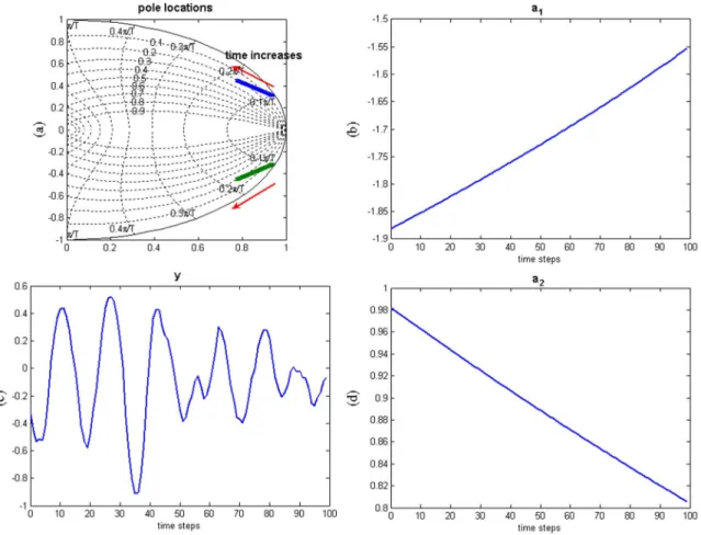
Fig. 1. Second-order AR system. (a) Pole locations. (b)a (k). (c) y(k). (d) a (k).
where . and ,
, denote the MAP estimates of and , respectively.
Then, and ’s are chosen to simplify (23). Let
(24)
(25) where is a positive real number which will be determined later and
Define the parameter estimation error of and to be
(26)
Substituting (24)–(26) into (23) and rearranging the equation, we end up with
(27) Combine (27) for all in a matrix form. Then
..
. ... ... . .. ...
..
. (28) Equation (28) gives the error of the MAP estimate provided that and ’s follow (24) and (25).
’s in (25) affecting the bias and variance of the estimated parameters. This is because large leads to small (25), which, in turn, introduces a “flat” distribution of (5). Con-sequently, it is likely that is very small and, therefore, is confined to a small neighborhood of . In other words, the estimated parameters have a smooth fluctuation but are not
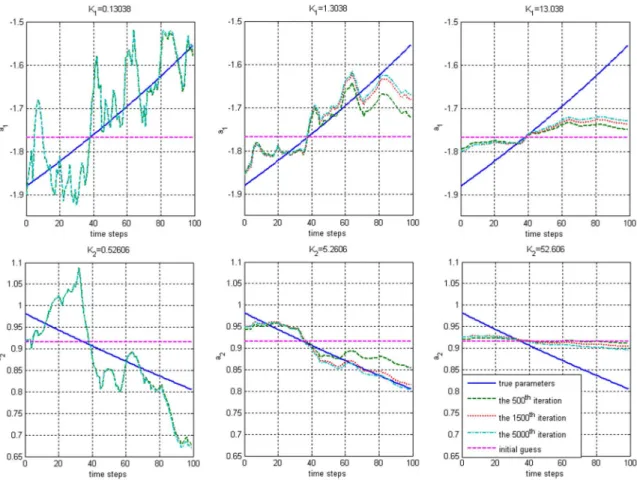
Fig. 2. Estimated parameters at various iterations. Left columnK = 0:13038 and K = 0:52606. Middle column K = 1:3038, K = 5:2606. In the right column,K = 13:038 and K = 52:606. The solid line (-) indicates true parameters. The dashed line (--) indicates the 500th iteration. The dotted line (.) represents the 1500th iteration and the dashed–dotted line (-.) is the 5000th iteration.
able to trace large variations of the true parameters. Hence, the bias is large.
It is not easy to find “optimal” ’s that achieve multiple con-flicting goals, such as fast convergence, small bias, and small variance of estimation; however, (28) suggests the following rule of thumb in selecting ’s. Namely choose ’s such that the norm of the right-hand side of (28) is as small as possible. The minimal 2-norm of takes place whenever is the orthogonal projection of in the direction of . Hence
(29) Note that (29) is not an optimal choice of in any sense. However, it is the author’s experience that such a choice gives rise to satisfactory results. Simulations in the next section verify this point of view.
Equation (29) requires the values of true parameters and the process noise . Both of them are not available. Therefore, they can be replaced by their respective estimated values as follows:
where is the estimate of at the th iteration while is the estimate of at the th iteration. How-ever, it has been found that frequent updating of may de-teriorate the performance. In this case, is updated every iterations, where is sufficiently large such that has con-verged within iterations.
IV. SIMULATIONS
In order to investigate the strengths and weaknesses of the proposed method, it is desirable to compare the performance of Algorithm I with those of other methods. However, it is be-yond the scope of this paper to conduct a comprehensive test of all kinds of time-varying system identification techniques. Sim-ulations have been conducted to show that the RLS algorithm (with forgetting factors) results in unsatisfactory performance in the case of fast-varying systems while Algorithm I still works properly; however, the comparisons with the RLS algorithm are skipped in this paper due to the limited space. Instead, a particle filter [27] is implemented in this section as a comparison of Al-gorithm I. Particle filtering is chosen because it also belongs to the category of stochastic methods; hence, the comparison can be made on a fair basis. Both Algorithm I and the particle filter are implemented by C++ language and executed on the same personal computer (with a 3-GHz Pentium 4 CPU). The execu-tion time and estimaexecu-tion errors of both methods are presented for comparison.
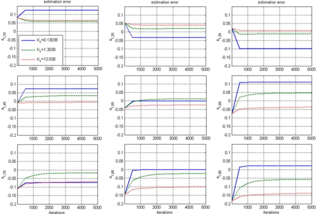
Fig. 3. Convergence of the estimation errors ofa (k) as the algorithm iterates for various K . The solid line (-) represents K = 0:13038. The dashed line (--) isK = 1:3038. The dotted line (.) is K = 13:038.
In this section, we consider a time-varying second-order AR system
(30) where is a zero mean white Gaussian noise with stan-dard deviation . Let the system’s instantaneous poles
be . Let and
. Thus,
and . Note that in this case, and are not independent, which violates the assumption of (4). However, the simulation results show that the Algorithm I still yields sat-isfactory estimation. The pole locations , parameters and , and the output are shown in Fig. 1 for
.
If this system is regarded as time invariant, the least-square estimates are and . Clearly, the least-square estimates are not able to capture the time-varying features of the AR system. Nevertheless, they can serve as the initial guesses of Algorithm I and the particle filter. Before implementing Algorithm I and the particle filter, we explain why the Markov Chain Monte Carlo (MCMC) method is not recommended in this case. A crucial step of the MCMC method is to draw samples of the unknown parameters in a del-icate way such that the probability distribution of these samples asymptotically approaches the desired posterior probability. However, it is not an easy task to design an efficient sampler due to the complexity of (11)–(13). The Gibbs sampler [23] is widely used in the case that the dimension of the parameter
space is high. Then, samples of each are drawn based on the conditional probability proportional to [(15) and (16)]. This can be achieved by drawing samples from (or ) directly and (or ) plays the role of the importance function [28]. However, as the length of the data increases, the high-probability regions of and diminish and do not overlap, which makes the importance sampling inefficient. Due to its low efficiency, the MCMC method will not be applied in this section.
A. Simulation Results of Algorithm I
For simplicity, fixed-value ’s are used in this section. Three sets of and are selected to investigate their effects on es-timation errors. According to (29), and
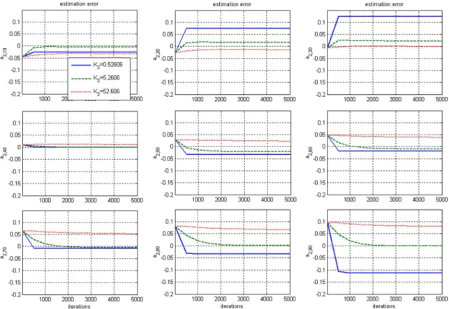
. The values of the other two sets of and are chosen to be the 10 and 1/10 times of the first set, respectively. Then, Algorithm I is applied to estimate and for . The results are shown in Fig. 2. The estima-tion errors of and at nine selected time points for various iterations are shown in Figs. 3 and 4, respectively. These figures illustrate the convergence rate of Algorithm I.
It is clear from the simulation that larger and result in smaller variations among the estimated parameters and slower convergence rate. If and are too large, the estimated pa-rameters are nearly constant for all . This observation coin-cides with the discussion in Section III-B. It is also observed that the values of ’s suggested by (29) yield satisfactory re-sults in terms of bias and variance of the estimation (see the middle column of Fig. 2).
Fig. 4. Convergence of estimation errors ofa (k) as the algorithm iterates for various K . The solid line (-) indicates K = 0:52606. The dashed line (--) is K = 5:2606. The dotted line (.) is K = 52:606.
TABLE I
SIMULATIONRESULTS OFALGORITHMI (AFTER5000 ITERATIONS)
TABLE II
SIMULATIONRESULTS OF THEPARTICLEFILTER
: Std denotes “standard deviation”
Simulation results are listed in Table I. The estimation error is defined as , , 2. It can be seen that the
’s suggested by (29) result in the smallest errors.
B. Simulation Results of the Particle Filter
The particle filter implemented in this section consists of the following steps.
Choose sample size and hyperparameters , , , 2, and .
Given initial values of , , 2, and .
For each , .
1) Draw samples of , , 2, and .
2) Draw samples of , , 2; .
3) .
4) Apply residual resampling if the effective sample size is smaller than the prescribed threshold [29].
5) , , 2, and
.
6) The estimated parameter at time step is , , 2.
The values of the hyperparameters are set to be the same as those in the Algorithm I (i.e., , ,
, and corresponding to
and ) [(24) and (25)]. Note that uncertainty exists in the estimates of the particle filter. Hence, for each sample size , we run the particle filter ten times. The average execution time for each run, and the mean and the standard deviation of
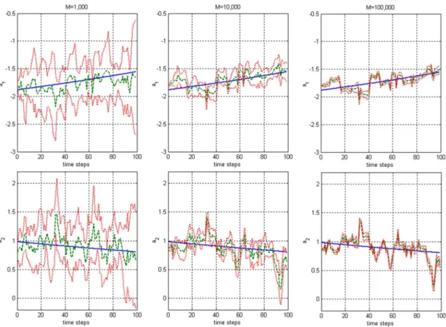
Fig. 5. Estimated parameters for various sample sizes. Left columnM = 1; 000. Middle column M = 10; 000. Right column M = 100; 000. Upper row a . Lower rowa . The solid line (-) represents true parameters. The dashed line (--) indicated estimated parameters. The dotted line (.) is the standard deviation of the estimated parameters.
the estimation errors are listed in Table II. Fig. 5 shows the true and estimated parameters.
C. Discussion
It can be seen from Table II that an increase of the sample size reduces the variances of the estimation errors, but has minor ef-fects on the average estimation errors. Comparing the results in Tables I and II, we found that Algorithm I achieves smaller esti-mation errors with less computation power. Moreover, the result of Algorithm I is deterministic (i.e., the same MAP estimate is obtained for every run provided that the same hyperparameters are used). On the other hand, the particle filter can perform on-line estimation of the parameters but the result is uncertain. A large sample size reduces the uncertainties; however, more com-putation power is required.
V. CONCLUSION
In this paper, the problem of identifying time-varying pa-rameters of autoregressive (AR) systems was investigated. It was formulated as a Bayesian inference problem with additional constraints imposed on the parameters in the form of condi-tional and prior probabilities. These constraints represent the objective knowledge or the subjective belief about the physical system; however, the conditional Gaussian distributions and the corresponding conjugate priors arise naturally if little about the system is revealed.
Based on the probabilistic assumptions, an efficient iterative algorithm was proposed to evaluate the maximum a posteriori (MAP) estimates of parameters. Simulation results showed that the proposed method has satisfactory performance. Compared with the particle filter, the proposed method achieved smaller estimation errors with less computation power.
In this paper, the order of the AR system is assumed to be known in advance. In reality, this information is usually not available. Determining the order of the identified system is called “model selection” in system identification literature. Cri-teria, such as Akaike’s Information Criterion (AIC), Bayesian Information Criterion (BIC), and final prediction error (FPE), have been proposed for linear time-invariant systems [5], but the model selection for time-varying systems remains an open question. Although the order of the time-varying system can be roughly estimated by the aforementioned criteria, assuming temporarily that the system is time invariant, there is no guar-antee that the correct model will be selected. Model selection for time-varying systems will be a future research topic.
In addition to the AR model, there are many other parametric representations of systems, such as ARX and ARMAX models [5]. In these cases, the “amount of information” contained in the input signal becomes an issue. If the information is not “rich” enough, only parts of the system’s characteristics will be acti-vated. However, a rigorous presentation of the identifiability of the time-varying system and the relation to the properties of the input–output signals requires more research effort in the future.
REFERENCES
[1] Y. Grenier, “Time-dependent ARMA modeling of nonstationary sig-nals,” IEEE Trans. Acoust., Speech, Signal Process., vol. ASSP-31, no. 4, pp. 899–911, Aug. 1983.
[2] R. A. Iltis and A. W. Fuxjaeger, “A digital spread-spectrum re-ceiver with joint channel and Doppler shift estimation,” IEEE Trans.
Commun., vol. 39, no. 8, pp. 1255–1267, Aug. 1991.
[3] A. Singhal and A. S. Kiremidjian, “Method for probabilistic evaluation of seismic structural damage,” J. Struct. Eng., vol. 122, pp. 1459–1467, 1996.
[4] J. P. Kaipio and P. A. Karjalainen, “Estimation of event-related syn-chronization changes by a new TVAR method,” IEEE Trans. Biomed.
Eng., vol. 44, no. 8, pp. 649–656, Aug. 1997.
[5] L. Ljung, System Identification: Theory for the User, 2nd ed. Upper Saddle River, NJ: Prentice-Hall, 1999.
[6] R. Johansson, System Modeling and Identification. Englewood Cliffs, NJ: Prentice-Hall, 1993.
[7] P. A. Ioannou and J. Sun, Robust Adaptive Control. Upper Saddle River, NJ: Prentice-Hall, 1996.
[8] K. Nishiyama, “AnH optimization and its fast algorithm for time-variant system identification,” IEEE Trans. Signal Process., vol. 52, no. 5, pp. 1335–1342, May 2004.
[9] J. C. M. Bermudez and N. I. Bershad, “Transient and tracking per-formance analysis of the quantized lms algorithm for time-varying system identification,” IEEE Trans. Signal Process., vol. 44, no. 8, pp. 1990–1997, Aug. 1996.
[10] R. Zou and K. H. Chon, “Robust algorithm for estimation of time-varying transfer functions,” IEEE Trans. Biomed. Eng., vol. 51, no. 2, pp. 219–228, Feb. 2004.
[11] M. K. Tsatsanis and G. B. Giannakis, “Time-varying system iden-tification and model validation using wavelets,” IEEE Trans. Signal
Process., vol. 41, no. 12, pp. 3512–3523, Dec. 1993.
[12] Y. Zheng, D. B. H. Tay, and Z. Lin, “Modeling general distributed non-stationary process and identifying time-varying autoregressive system by wavelets: Theory and application,” Signal Process., vol. 81, pp. 1823–1848, 2001.
[13] K. B. Eom, “Analysis of acoustic signatures from moving vehicles using time-varying autoregressive models,” Multidimensional Syst.
Signal Process., vol. 10, pp. 357–378, 1999.
[14] K. B. Eom, “Nonstationary autoregressive contour modeling approach for planar shape analysis,” Opt. Eng., vol. 38, pp. 1826–1835, 1999. [15] G. N. Fouskitakis and S. D. Fassois, “On the estimation of
nonsta-tionary functional series TARMA models: An isomorphic matrix algebra based method,” J. Dyn. Syst., Meas. Control, vol. 123, pp. 601–610, 2001.
[16] M. K. Tsatsanis and G. B. Giannakis, “Subspace methods for blind es-timation of time-varying FIR channels,” IEEE Trans. Signal Process., vol. 45, no. 12, pp. 3084–3093, Dec. 1997.
[17] K. B. Eom, “Time-varying autoregressive modeling of high range res-olution radar signatures for classification of noncooperative targets,”
IEEE Trans. Aerosp. Electron. Syst., vol. 35, no. 3, pp. 974–988, Jul.
1999.
[18] A. Doucet, S. J. Godsill, and M. West, “Monte Carlo filtering and smoothing with application to time-varying spectral estimation,” pre-sented at the IEEE Int. Conf. Acoustics, Speech Signal Processing II, Istanbul, Turkey, 2000.
[19] S. J. Godsill, A. Doucet, and M. West, “Monte Carlo smoothing for nonlinear time series,” J. Amer. Statist. Assoc., vol. 99, pp. 156–168, 2004.
[20] S. Godsill and T. Clapp, “Improvement strategies for Monte Carlo particle filters,” in Sequential Monte Carlo Methods in Practice, A. Doucet, N. D. Freitas, and N. Gordon, Eds. Berlin, Germany: Springer, 2001, pp. 139–158.
[21] J. M. Bravo, T. Alamo, and E. F. Camacho, “Bounded error identifi-cation of systems with time-varying parameters,” IEEE Trans. Autom.
Control, vol. 51, no. 7, pp. 1144–1150, Jul. 2006.
[22] V. Gemez and A. Maravall, “Estimation, prediction, and interpolation for nonstationary series with the Kalman filter,” J. Amer. Stat. Assoc., vol. 89, pp. 611–624, 1994.
[23] C. P. Robert and G. Casella, Monte Carlo Statistical Methods. Berlin, Germany: Springer, 2004.
[24] J. M. Bernardo and A. F. M. Smith, Bayesian Theory. New York: Wiley, 2000.
[25] R. E. Neapolitan, Learning Bayesian Networks. Upper Saddle River, NJ: Prentice-Hall, 2004.
[26] M. Vidyasagar, Nonlinear Systems Analysis, 2nd ed. Englewood Cliffs, NJ: Prentice-Hall, 1993.
[27] S. Arulampalam, S. Maskell, N. Gordon, and T. Clapp, “A tutorial on particle filters for on-line non-linear/non-Gaussian Bayesian tracking,”
IEEE Trans. Signal Proces., vol. 50, no. 2, pp. 174–188, Feb. 2002.
[28] C. Andrieu, N. D. Freitas, A. Doucet, and M. I. Jordan, “An introduc-tion to MCMC for machine learning,” Mach. Learn., vol. 50, pp. 5–43, 2003.
[29] J. S. Liu and R. Chen, “Sequential Monte Carlo methods for dynamic systems,” J. Amer. Stat. Assoc., vol. 93, pp. 1032–1044, 1998.
Tesheng Hsiao (M’05) received the B.S. and M.S.
degrees in control engineering from National Chiao Tung University, Hsinchu, Taiwan, R.O.C., in 1995 and 1997, respectively, and the Ph.D. degree in mechanical engineering from the University of California, Berkeley, in 2005.
Currently, he is an Assistant Professor in the Department of Electrical and Control Engineering at National Chiao Tung University. His research interests include advanced vehicle-control systems, fault detection and fault-tolerant control, and system identification.