Exploiting fine-grain parallelism in the H.264 deblocking filter by
operation reordering
Tsung-Hsi Weng
∗,
Chung-Ping Chung
Department of Computer Science, National Chiao Tung University, Engineering Building C, Kuang-Fu Campus, 1001 University Road, Hsinchu 300, Taiwan, ROC
a r t i c l e i n f o Article history:
Received 16 April 2012 Received in revised form 13 July 2013
Accepted 14 October 2013 Available online 22 October 2013
Keywords: Deblocking Parallelization Data intensive Many-core architecture H.264
a b s t r a c t
In the H.264 video compression standard, the deblocking filtering contributes about one-third of all com-putation in the decoder. With many-core architectures becoming the future trend of system design, computation time can be reduced if the deblocking appropriately apportions its operations to multiple processing elements. In this study, we used a four-pixel-long boundary as the basis for analyzing and exploiting possible parallelism. Compared with the two-dimensional (2D) wavefront method order for deblocking both 1920×1080- and 1080×1920-pixel frames, the proposed design exhibits speedups of 1.92 and 2.44 times, respectively, given an unlimited number of processing elements. Compared with our previous design, it gains speedups of 1.25 and 1.13 times, respectively. In addition, as the frame size grows, this approach requires only extra time that is proportional to the square root of the frame size in-crease (keeping the same width to height ratio), pushing the boundary of practical real-time deblocking of increasingly larger video sizes.
© 2013 Elsevier B.V. All rights reserved.
1. Introduction
Integrated circuit capacity on a single die has increased as pre-dicted by Moore’s Law in the past 50 years. However, single-thread computing performance has been observed to level off in past decades, due to both insufficient parallelism in applications and power usage limitations. Multi-core and many-core designs allow not only efficient use of energy, but also parallel processing capa-bilities at almost all levels, pushing the computation power of a single die up at a rate proportional to IC technology.
We study how to explore multi-core hardware capabilities in intensive computing. The paradigm of pervasive data-intensive computing has become widely applied in all computer devices especially for multimedia processing. In this paper, we choose H.264 to be the target application as it is a widely used tech-nique for such multimedia processing that is highly computation and data intensive. H.264 provides acceptable image quality and a reduction in bit rate compared to the existing video compression standards. In addition, it provides high adaptability and superior error resilience for a wide range of multimedia applications [1]. Due to H.264’s intensive data compression, picture frame deblock-ing is a crucial process and is our focus.
Deblocking is intended to smoothen block-edge artifacts caused by the decoding process and enhance picture quality. In the
∗Correspondence to: No.17, Ln. 106, Minzu Rd., Xinying Dist., Tainan City 730,
Taiwan, ROC. Tel.: +886 952767833; fax: +886 35715460.
E-mail addresses:[email protected](T.-H. Weng),
[email protected](C.-P. Chung).
encoding process, the H.264 encoder uses the macroblock (MB), a 16
×
16 pixel square, as the basic coding unit. The quantiza-tion of the macroblocks causes visual discontinuities between the edges of the decoded macroblocks. The pixels located on the mac-roblock boundaries with a similar value might be decoded with a larger difference in values for the aforementioned reason, resulting in a decline in picture quality. Therefore, the purpose of deblock-ing is to smoothen block artifacts caused by the decoddeblock-ing process to enhance picture quality. Another advantage of deblocking is to increase coding efficiency. Decoded and deblocked images are ref-erenced later, and because the picture is of superior quality, the encoded bit rate is reduced.Deblocking filtering accounts for one-third of all computation in a decoder [2]. Many-core architectures are becoming the trend; if deblocking can be processed using a multi-core parallel processing architecture, processing can be distributed to different computing PEs to address and reduce the execution time. Whereas most paral-lel processing of deblocking currently focuses on paralparal-lelization at the MB level, we found that parallelizing deblocking at a granular-ity of 16-pixel-long boundaries enables more parallelism than par-allelization at the MB level in our previous work [3]. In this paper, we further examine the possibility of parallelizing deblocking at a finer granularity and whether it can be developed according to our presented design. We analyze the deblocking order to obtain the dependency between the various boundaries and then propose an execution order in which the execution of deblocking in this order provides improved parallelism.
The remainder of this paper is organized as follows. Section2
introduces the background of the deblocking filtering and related
0167-739X/$ – see front matter©2013 Elsevier B.V. All rights reserved.
Fig. 1. (a) Affected pixels in deblocking. (b) The pixel values before deblocking; the P0–P3 and Q0–Q3 pixel value gap causes a visual discontinuity. (c) After deblocking; the pixel values are now smooth.
a
b
Fig. 2. Deblocking orders of (a) intra-MB and (b) inter-MB.
work for deblocking parallelization. Section3shows our paral-lelized design. Section 4 presents an analysis of the proposed method and compares it with related works. Section5shows our proposed hardware architectural requirements. Finally, the con-clusion and suggestions for future research are provided.
2. Background and related studies
2.1. Background
The deblocking filtering is used to smoothen block-edge arti-facts.Fig. 1(b) shows a block-edge artifact caused by a large differ-ence in pixel values. The pixels P0–P3 and Q0–Q3 inFig. 1(b) can be located either vertically or horizontally, as shown inFig. 1(a). Deblocking applied on the P0–P3 and Q0–Q3 pixel values enables these eight values to appear visually smooth. The pixel value dis-tribution after deblocking is shown inFig. 1(c).
Deblocking is needed for both MB boundaries and 4
×
4 block boundaries. Because the MB is the basic coding unit in H.264, block-edge artifacts occur easily at MB boundaries. In addition, some coding modes use 4×
4 blocks for inter prediction and intra prediction. For these cases, deblocking is needed to smoothen the block-edge artifacts.The MB deblocking internal (intra-MB) execution order, as defined by the H.264 standard, is shown inFig. 2(a). The execution starts by deblocking a column of pixels moving horizontally from left to right, and then a row of pixels moving vertically from top to bottom. The inter-MB execution order is shown inFig. 2(b), and moves from left to right and top to bottom.
Although the H.264 standard defines the deblocking order as shown inFig. 2, the order can be altered if the final decoding re-sults are correctly outputted. Altering the order in which the cal-culation is performed is an opportunity for parallelizing deblocking filtering. We propose a conceptual design to improve the paralleliz-ability of the deblocking.
2.2. Related work
Pipelining the H.264 video decoding stages and distributing the workload to threads working on different cores are effective meth-ods to make use of the system-provided parallelism in a multi-core system. Several studies [4–8] have focused on this domain. T.W. Chen et al. [6] arranged the H.264 decoder functions into proper pipelining schedules. Y.K. Chen et al. [7] provided an ef-ficient multi-threaded H.264 encoding/decoding method on Intel hyper-threading architecture. H. Baik et al. [4] exploited function-level parallelism (FLP) on IBM CELL architecture. Moreover, Y. Kim et al. [8] optimized the performance of [4] using dynamic load balancing. Furthermore, K. Nishihara et al. [5] provided a flexi-ble partitioning of the H.264 decoding functions for an embedded multi-core processor.
However, because microprocessor design increasingly involves applying fully customized PEs for higher computing performance and energy efficiency [9,10], another dimension of parallelism is needed to extend the use of the provided computation resource. Consequently, various designs [11–16] focus on the data-level par-allelism (DLP) of the H.264 codec. In recent years, several methods [17,18] have considered both FLP and DLP to exploit both dimen-sions of parallelism. Today, DLP is increasingly crucial.
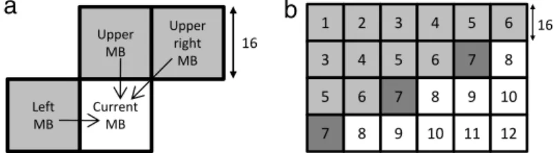
The two-dimensional (2D) wavefront method [11] proposed by Van Der Tol et al. exploits DLP by using the MB as a unit for paral-lelization. InFig. 3(a), according to the deblocking order, the cur-rent MB has a data dependency on the upper, upper-right and left MBs. Therefore, when using an MB as the parallelization unit, the upper, upper-right and left MBs must be deblocked before the cur-rent MB. InFig. 3(b), the MBs that can be processed simultaneously are numbered together.
S. Sun [13] proposed a macroblock region partition (MBRP) to further use the 2D wavefront method. The video encoder of this de-sign partitions one frame into individual coded regions, and each region can apply the 2D wavefront method individually. Moreover, F.H. Seitner et al. [15] evaluated various types of partitioning ap-proaches including the multi-column, parallel, rotating slice-parallel, and diagonal approaches. However, this enhancement requires a video stream that is not compatible with the H.264 stan-dard. In addition, K. Schöffmann [12] mentioned that increasing the number of partitions also increases the bit rate requirements of the H.264 video.
The three-dimensional (3D) wavefront method [14] is based on the 2D wavefront method; however, it also uses inter-frame parallelism, meaning that more MBs can be processed in parallel. This method can considerably enhance the parallelism. A. Azevedo et al. [16] implemented the 3D wavefront method on a multi-core
Fig. 3. (a) Data dependencies in inter-MB deblocking. (b) MBs that can be processed simultaneously.
a
b
Fig. 4. (a) ID assignment and (b) data dependency of an MB.
architecture composed of NXP TriMedia TM3270 embedded pro-cessors to verify its effects in a real-world scenario.
In our previous work [3], we found that parallelizing deblock-ing at a granularity of 16-pixel-long boundaries produces more parallelism than parallelization at the MB level. As mentioned, de-blocking at a finer granularity might enable rapid attainment of the maximal parallelism, but also benefit diminishing the limitation from the shape of the frame.
The 3D wavefront method is compatible with MB-level meth-ods and our previous work. The MB-level methmeth-ods and our previ-ous work are used for intra-frame parallelization, whereas the 3D wavefront method is used for inter-frame parallelization. In the fol-lowing sections, we explain whether deblocking at a finer granu-larity can increase the amount of parallelism and still be combined with the 3D wavefront method to further increase the parallelism.
3. Design
Analyzing applications at a finer granularity usually provides additional opportunities for parallelization. In H.264, the standard defined orders intersect with each other on a 4
×
4 grid; thus, we used four-pixel-long boundaries as the basic unit. In the follow-ing section, we first analyze the data dependencies and generate the corresponding data dependency chain. Second, we determine the critical paths of the data dependency chain and assign the de-blocking order of four-pixel-long boundaries on the critical paths based on their dependency depth. Last, we determine the order of deblocking the four-pixel-long boundaries that are not on the crit-ical paths based on the optimal use of the provided hardware re-sources. At the end of this section, we consider the assignment of available PEs.3.1. H.264 deblocking data dependency tree
To delineate the data dependency chain, we assigned IDs (b1–b32) to each of the four-pixel-long boundaries in an MB
(Fig. 4(a)). The result of deblocking b5 became an input into the
deblocking for b6, and that result subsequently became the inputs
for both b1and b7, and so on. In accordance with the data
depen-dencies caused by the standard H.264 order, the data dependency chain for intra-MB deblocking is as shown inFig. 4(b).
Moreover, the data dependency tree can be derived for deblock-ing in an MB, as shown inFig. 5.
InFig. 5, the data dependency tree is represented as eight timing phases. The timing of each boundary signifies the earliest time that the deblocking can operate. The black solid arrows mean that these inputs resulted from other four-pixel-long boundaries that are in the same MB; the black dotted arrows represent the inputs result-ing from four-pixel-long boundaries that are in different MBs; and the double arrows mean that the inputs are used for the first time and originate from the external memory. The inter-MB depen-dency tree can be constructed by placing MBs side by side and link-ing the black dotted arrows (which are shown inFig. 5) together.
3.2. Deblocking order of four-pixel-long boundaries on the critical paths
The critical paths of the data dependency tree must be deter-mined in the next step. When deblocking a critical path, this de-blocking time determines the performance. The three steps, which are outlined below, are used to illustrate the critical paths of a frame.
Step 1: Identify critical paths among four-pixel-long boundary data dependency chains in MB.
A frame containing only one MB was assumed.Fig. 6, which is a trivial derivation fromFig. 5, shows the critical paths of this frame with arrows representing the data dependency directions. By or-dering the counts of arrows from b5to each four-pixel-long
bound-ary, the execution order of the critical paths could be generated. Step 2: Identify critical paths among four-pixel-long boundary data dependency chains in the same row of MBs.
Following Step 1, we extended the analyzed frame size to one row of m MBs.Fig. 7shows the critical paths of this frame with three types of arrows. The gray arrows (from Step 1) indicate intra-MB dependencies. The double arrows indicate inter-MB de-pendencies in a row of MBs. The black dotted arrows indicate some intra-MB dependencies not shown inFig. 5. These intra-MB depen-dencies are added because of the effects of inter-MB dependepen-dencies. To meet the order demanded by the critical paths, we modified the deblocking order of Step 1, as shown inFig. 8. The modifica-tion is represented by the numbers in bold, which are on the ex-tra critical paths caused by the inter-MB dependencies in a row of MBs. Though not every critical path that resides in different MBs is identical, this order fulfils the requirements and maintains reg-ularity.Fig. 9shows the order of two adjoining MBs in the same row of MBs. Note that the deblocking of the adjoining MB on the right starts at Time 7, which precedes the last operation of the MB on the left. The performance improvements are analyzed further in the analysis section.
Step 3: Identify critical paths among four-pixel-long boundary data dependency chains in adjoining rows of MBs.
In this step, we extended the size of a frame to n rows of m MBs.
Fig. 10shows the corresponding critical paths. The gray arrows in-dicate both the intra-MB and the same row of inter-MB data de-pendencies. The black arrows indicate data dependencies between adjoining rows of MBs. Moreover, the distribution of critical paths forms eight types of MBs. To meet the requirements of these criti-cal paths, we provided the deblocking order extended from Step 2 inFig. 11.
The only modification made is shown inFig. 11by the number 3 in bold, which is on the extra critical path caused by adjoining rows
Fig. 5. Data dependency tree of an MB.
a
b
Fig. 6. (a) Critical paths of a frame with only one MB and (b) deblocking order on critical paths.
of MBs.Fig. 12illustrates the deblocking order of a 3 MB
×
3 MB frame, which is the smallest example containing all eight types of MBs shown inFig. 10. By labeling the start of the first row of MBs as the first stage, we found that the second row of MBs started de-blocking at the sixth stage. The analysis of the performance im-provements is also discussed in the analysis section.3.3. Deblocking order of four-pixel-long boundaries on the non-critical paths
The deblocking order inFig. 11fulfils the requirements for cor-rect deblocking of all four-pixel-long boundaries on the critical paths. Next, we determined the execution order of the boundaries that are not on the critical paths. Because these boundaries are not on the critical paths, a degree of flexibility is possible in reordering, while not increasing the time for deblocking.Fig. 13shows all the possible orders for four-pixel-long boundaries not on critical paths without increasing the length of any critical path. These boundaries were categorized into three groups. By following the arrows in each
Fig. 8. Deblocking order fulfils the critical paths of a single row of MBs.
group, all possible orders can be generated. Taking the group con-taining b8
,
b12, and b16 for example,{
4,
5,
6}
, {
4,
5,
7}
, {
4,
6,
7}
,and
{
5,
6,
7}
are all the possible order assignments for{
b8,
b12,
b16}
in this group.
When we considered all the possible order assignments for the boundaries not on the critical paths, we found that different order assignments result in different amounts of required PEs. To minimize the total amount of required PEs, we had to derive the minimal possible amount of required PEs for one additional MB row. Although deblocking one MB requires at least eight time units because of the length of the critical paths in a single MB, we found that spanning one MB horizontally used only six more stages in the critical paths according to the order for four-pixel-long boundaries, as shown in Fig. 12. Moreover, one MB contains 32 boundaries requiring deblocking, and had to be completed in six time units. Assuming that one PE could deblock one four-pixel-long boundary in a single time unit, the minimal possible amount of required PEs
Fig. 9. Deblocking order of boundaries on critical paths in one row of MBs.
Fig. 10. Critical paths of a frame with m×n MBs.
Fig. 11. Deblocking order that fulfils the critical paths of a frame with m×n MBs.
for one MB row without increasing the execution time is a ceiling of 16
/
3.Because of this minimal amount of required PEs for one MB row, we proposed a specific order, which is shown inFig. 14(a). A regular number sequence of the number of boundaries exists that could be deblocked in parallel: 12
(
565565)
∗565553 (Fig. 14(b)). This orderrequired seven PEs for one MB row, which is exactly the ceiling of 16
/
3. In addition, deblocking n rows of MBs uses only a ceiling of 16n/
3 PEs, which is also the minimal possible amount without increasing the execution time (Fig. 15).3.4. Assignment of processing elements
Because of the relationship between the number of PEs and the aspect ratio of the frame to be deblocked, two cases can result: Case I: Degree of parallelism depends on the frame’s aspect ratio.
Assuming that more PEs are available than needed, the degree of parallelism is limited only by the frame aspect ratio. Whereas processing 16 pixels horizontally (the width of one MB) occurs in
Fig. 12. Deblocking order of boundaries on critical paths in a 3 MB×3 MB frame. All eight types of MBs are shown in this example.
six stages, processing 16 pixels vertically occurs in only five stages in the proposed order. Consequently, deblocking the first row of MBs finishes before starting the last row of MBs when the number of rows of MBs is less than (6
/
5)×
(the number of columns of MBs in a frame). We categorized the effects of the frame’s aspect ratio into the following two situations:i. Number of rows of MBs in a frame
≤
6/
5×
number of columns of MBs in a frame (degree of parallelism limited by the number of rows of MBs in a frame).In this situation, the number of rows of MBs in the frame dom-inates the maximal parallelism. According to the deblocking order inFig. 15, the maximal parallelism of three rows of MBs is 16. We found that the maximal parallelism of one row of MBs is a ceiling (16
/
3). For example, the maximal parallelism of one row of MBs is 6, the maximal parallelism of two rows of MBs is 11, and the maximal parallelism of three rows of MBs is 16. Our method has a wind-up and wind-down time similar to that of the 2D wavefront method.Fig. 16shows the portions of a frame during the wind-up and wind-down time. The upper-left gray region shows the start-ing up of the deblockstart-ing and the lower-right gray region is the fin-ishing of the deblocking. In these regions, the deblocking could not reach the maximal parallelism. The white region is where the de-blocking could reach the maximal parallelism. The degree of par-allelism and timing relationship diagram is shown inFig. 17. ii. Number of rows of MBs in a frame>
6/
5×
number of columns of MBs in a frame (degree of parallelism limited by the number of columns of MBs in a frame).In this situation, which is shown inFig. 18(a), the degree of par-allelism is equal to the ceiling (16
/
3) multiplied by the number of rows of MBs that can start deblocking before the deblocking for the first row of MBs completes. As explained at the beginning of Case I, if the ratio of the height to width is larger than 6/
5, the degree ofFig. 13. Flexible orders on non-critical-path boundaries.
Fig. 14. Proposed deblocking order and the number of boundaries deblocked in parallel for one MB row.
parallelism is limited by the frame width. The degree of parallelism and timing relationship diagram is shown inFig. 18(b).
Case II: the number of PEs is insufficient to exploit maximal paral-lelism.
In this case, the frame has to be split into multiple stripes for deblocking. We assumed that a limited number of PEs are available, such that only K rows of MBs could be deblocked simultaneously, where K is inferior to the maximal number of parallelizable MB rows. Each stripe contains at most K parallelizable MB rows. In this instance, we first outlined a base approach and then proposed an improved one.
i. Base approach:
AsFig. 19shows, the frame is split into stripes where each stripe contained K rows of MBs. The execution order of the stripes is from top to bottom. We found that each stripe has a up and wind-down time, meaning that not all PEs can be busy during these times. The degree of parallelism and timing diagram is shown in
Fig. 20.
ii. Improved approach:
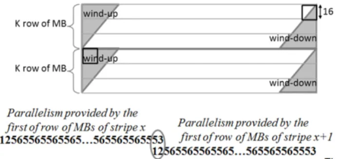
In the base approach, not all PEs can be busy during the wind-up and wind-down time in stripe deblocking, as shown inFig. 21(a). Notice that the execution of the wind-down of stripe x and the wind-up of stripe x
+
1 could be overlapped to fully utilize the PEs. Once a PE is available, stripe x+
1 could start deblocking immediately.Fig. 22shows how the first MB row of stripe x+
1 could start deblocking at the last two stages of deblocking the first MB row of stripe x as an example. Using this approach, the wind-up of stripe x+
1 could start the execution earlier than that in the base approach, as shown inFig. 21(b). Moreover, we maintained the regularity of the amount of required PEs for both stripes.Fig. 16. Portions of a frame during the wind-up and wind-down of deblocking order.
Fig. 17. The degree of parallelism and time relationship diagram.
By applying this method, we found the degree of parallelism and timing shown inFig. 23, which exhibits a reduction in the idle time of PEs. In addition, when the number of rows per stripe K does not divide evenly into the total number of MB rows, the final stripe has a number of idle PEs, as shown inFig. 24.
4. Simulation and modeling
The proposed order, subsequently called the Order4method,
was outlined in the previous section. In this section, the focus is on determining the degree to which this design can improve the parallelism and execution time. In this section, we first construct figures to show the benefits from the stripe overlapping in Order4,
Fig. 18. (a) The degree of parallelism is limited when the frame height is larger than 6/5 times of the frame width. (b) The degree of parallelism and timing relationship diagram.
Fig. 19. The number of PEs is insufficient to exploit maximal parallelism, frame split into multiple stripes for deblocking.
Fig. 20. The degree of parallelism and timing diagram when the number of PEs is insufficient to exploit maximal parallelism.
our previous work (subsequently called the Order16method), and
the 2D wavefront method. Second, we compare the effects of the three methods on both the horizontally shaped and the vertically shaped frames. Third, we illustrate situations where the Order4
outperformed the other two methods with an unlimited amount of
PEs and where it failed with a limited amount of PEs. In addition, we explain that our design also complements the 3D wavefront method. Moreover, we model the parallelism and time of deblock-ing a frame for all three methods to help choose a suitable order based on the shape of a frame and the number of available PEs. Fi-nally, we estimate the increase of the internal buffer space demand as well as the memory bandwidth requirements for deblocking.
4.1. Effects of stripe overlapping
To demonstrate the effects of the number of PEs and the benefits from overlapping the deblocking of adjoining stripes of MBs, we wrote a simulator to simulate the deblocking orders with or without overlapping for the 2D wavefront, Order16, and Order4
methods. We normalized the abilities of a PE and the basic time unit to those used in Section3for fair comparison.Fig. 25(a)–(c) show the effect of stripe overlapping on the total execution time for each method for a 1920
×
1080 frame size.First, we found that, for all these methods, the total execution time curves display a step-like pattern. This characteristic origi-nated from the splitting of frames. When the number of PEs ex-ceeds a threshold in which the number of PEs can be divided evenly into the total number of MB rows, the total execution time is greatly reduced, thus forming the curves.
Secondly, the stripe overlapping made the increase of the num-ber of PEs more beneficial than that without the stripe overlap-ping because the stripe overlapoverlap-ping could greatly prevent PEs from idling away during the wind-up and wind-down time of stripes. In addition, the 2D wavefront method gained the greatest benefit from stripe overlapping among the three methods because of long wind-up and wind-down times.
Fig. 21. (a) The degree of parallelism and timing relationship between stripe x and stripe x+1 before overlapping. (b) The degree of parallelism and timing relationship between stripe x and stripe x+1 after overlapping.
Fig. 22. PE assignment for the first MB row of both stripe x and x+1.
Fig. 23. Time reduction of improved approach.
Fig. 24. The degree of parallelism and timing relationship when the number of rows per stripe K does not divide evenly into the total number of MB rows.
4.2. Effects of different orders
To further compare the Order4 method with the Order16and
the 2D wavefront methods, Fig. 26shows a comparison of the execution time and number of PEs required of all three methods with stripe overlapping for both a horizontally shaped frame (1920
×
1080) and a vertically shaped frame (1080×
1920).We observed that, for all the three methods, using a large num-ber of PEs decreased the time to deblock a frame until the maximal parallelism of each method was exploited. Whereas the speedup of the 2D wavefront method stopped at 240 PEs for the horizontally shaped frame and at 136 PEs for the vertically shaped frame, the speedup of the Order16method kept improving until 272 PEs for
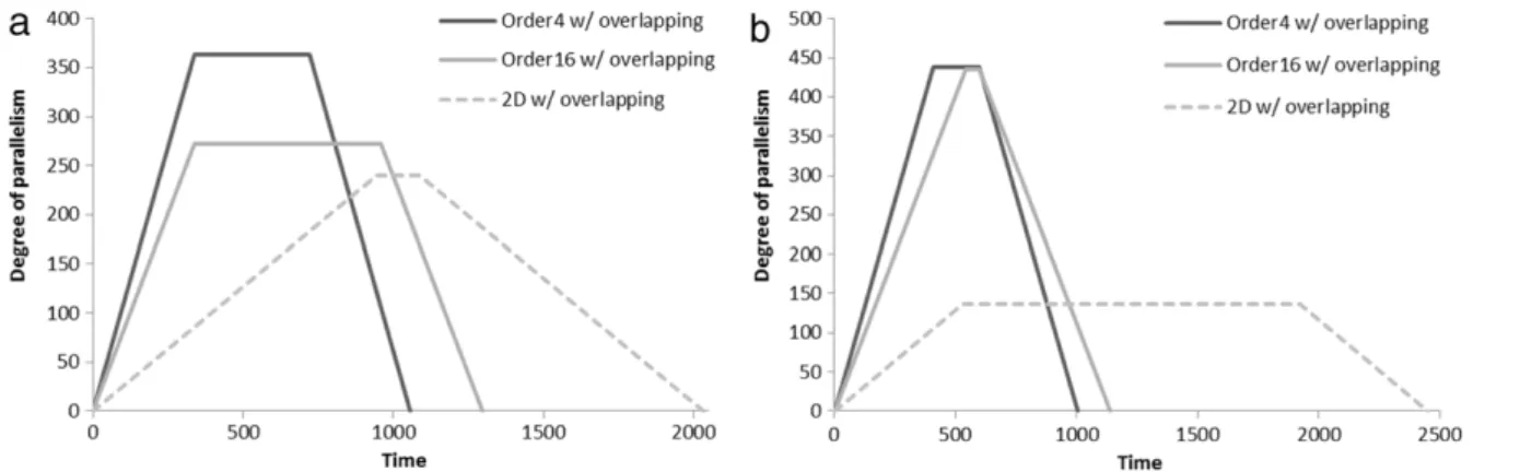
the horizontally shaped frame and 436 PEs for the vertical frame. Conversely, the Order4method kept improving until 363 PEs for
the horizontally shaped frame and 438 PEs for the vertically shaped frame.Fig. 27shows the comparison among these three methods with an adequate number of PEs for both (a) horizontally and (b) vertically shaped frames. The Order4method obtained the greatest
benefits of the three methods because of its shorter wind-up and wind-down time requirements, especially for the vertically shaped frame.
However, the time reduction of the 2D wavefront and Order16
methods was superior when the amount of PEs was significantly less than the maximal parallelism.Fig. 28shows the comparison of both the 2D wavefront and Order4 methods with deblocking
overlapping for a 1920
×
1080 frame using 70 PEs. This is an example of the Order4method displaying a higher maximal degreeof parallelism but failing to obtain a superior time reduction. When
In this section, we model the maximal parallelism being ex-ploited, the wind-up and wind-down time, and the total execu-tion time using algebraic equaexecu-tions. Although the Order4method
gained the greatest time reduction among the three methods when using unlimited PEs, it was less adequate than the 2D wavefront and Order16methods when the amount of PEs was limited. Using
these equations, we find the most suitable method based on the shape of the frame and the amount of available PEs.
Let
MH
=
the (given) number of rows of MBs in a frame; MW=
the (given) number of columns of MBs in a frame; N=
the (given) number of available PEs;TMB
=
time required to process one MB (changes with methods);Tdr
=
time delay between processes in the next row of MBs(changes with methods);
Prow
=
average number of required PEs to process one row of MBswithout prolonging the critical paths (changes with methods);
α =
the slope of average progress on a frame=
TMB/
Tdr;β =
the time taken to reach the maximal parallelism in one row of MBs (changes with methods);γ =
the time after reaching the maximal parallelism in one row of MBs (changes with methods).Then,
RF
=
the maximal number of rows of MBs that can be deblocked in parallel=
Min(
MH, ⌈α ×
MW⌉
)
(1)RP
=
the maximal number of rows of MBs that can be deblocked in parallel using N PEs=
Min
RF,
N Prow
(2)Rl_stripe
=
the number of rows of MBs in the last stripe(
if striped)
=
RFmod RP
,
if RFmod RP̸=
0RP
,
otherwise (3)P
=
the maximal parallelism= ⌈
RP×
Prow⌉
(4)Wind-up time TWind-up
=
the time taken to reach the RP-th MB row+
the time taken to reach the maximal parallelism in that MB row=
Tdr×
(
RP−
1) + β
(5)Wind-down time TWind-down
=
Time after finishing the last RPth row of MBs
.,
if PEs are sufficient
Time after finishing 1st row of MBs in last stripe
.,
if limited PEs=
Tdr×
(
Rp−
1) +
X,
if N≥ ⌈
Prow×
RF⌉
Tdr
×
(
# of rows in last stripe-1) +
Y,
if N< ⌈
Prow×
RF⌉
Fig. 25. Overlapping compared with non-overlapping in time for deblocking and number of PEs when frame size is 1920×1080. The time unit is the time required for deblocking a four-pixel-long boundary.
Fig. 26. Comparison among Order4, Order16, and 2D wavefront methods in time for deblocking and number of PEs when frame sizes are (a) 1920×1080 and (b) 1080×1920.
The time unit is the time required for deblocking a four-pixel-long boundary.
Fig. 27. Comparison among Order4, Order16, and 2D wavefront methods in degree of parallelism and time for deblocking when frame sizes are (a) 1920×1080 and
parallelism and time for deblocking when frame sizes are 1920×1080 and using 70 PEs.
=
Tdr×
(
Rp−
1) + γ ,
if N≥ ⌈
Prow×
RF⌉
Tdr×
(
Rp−
1) + γ ,
if N
< ⌈
Prow×
RF⌉
and Rl_stripe=
RF Tdr×
((
MHmod Rp) −
1) + γ ,
if N
< ⌈
Prow×
RF⌉
and Rl_stripe̸=
RF=
Tdr×
(
Rp−
1) + γ ,
if N≥ ⌈
Prow×
RF⌉
or Rl_stripe=
RF Tdr×
((
MHmod Rp) −
1) + γ ,
otherwise (6)where X is the time after the maximal parallelism in the last RPth row of MBs and Y is the time after the maximal parallelism in the first row of MBs in last stripe; both are equal to
γ
.Total Execution TimeTExec
=
the time taken before the last row of MBs starts
+
the time taken to finish the last row of MBs,
if PEs are sufficient(
the time to finish one row of MBs)
×
(
the number of pieces)
+
wind-down time of last stripe,
if limited PEs=
TMB×
MW+
Tdr×
(
MH−
1) + γ ,
if N≥ ⌈
Prow×
RF⌉
TMB×
MW×
MH RP
+
Tdr×
(
Rp−
1) + γ ,
if N
< ⌈
Prow×
RF⌉
and Rl_stripe=
RF TMB×
MW×
MH RP
+
Tdr×
((
MHmod RP) −
1) + γ ,
if N
< ⌈
Prow×
RF⌉
and Rl_stripe̸=
RF.
(7)
All these equations can be applied to the Order4
,
Order16, and2D wavefront methods using appropriate coefficients. The coeffi-cients that change with these methods are TMB
,
Tdr,
Prow, β
, andγ
. The sets of coefficients for each method are shown inTable 1, where the time unit is the time required for deblocking a four-pixel-long boundary.4.4. Internal buffer space demand increase
Applying the proposed order to the existing decoder increases the internal buffer. For a decoding method with an identical par-allelism at every stage of decoding, the temporal results could be directly bypassed into the following stages. The sizes of the internal buffers between the stages were minimized in this case.
In the video decoding pipeline, throughputs of different stages should be the same in a long run. However, speed fluctuation be-tween adjoining stages necessitates the use of an internal buffer.
2D wavefront 8 16 4 0 0
Order16 8 5 4 0 0
Order4 6 5 16/3 2 2
Where the time unit is normalized to the time required for deblocking a four-pixel-long boundary.
This happens to be the case if we replace the 2D wavefront deblock-ing algorithm and plain implementation with our scheme.Fig. 29
shows the block diagram when the Order16or Order4is used.
Be-cause the parallelisms of all the stages involved in the 2D wavefront method are the same, we joined all the processes occurring before the deblocking stage to simplifyFig. 29. To determine the buffer size, we show the snapshot of when our scheme begins exploiting maximal parallelism. At this instant, the stage before the deblock-ing stage is at its full speed as always, and the deblockdeblock-ing stage us-ing the Order4or Order16has just caught up. This is then the time
the maximal amount of decoded information needs to be buffered.
Fig. 30(a) shows the portion of a frame that has been decoded at this instant,Fig. 30(b) shows the portion of a frame that has been deblocked, andFig. 30(c) shows the portion of decoded frame that should be preserved. Note that this buffering is inevitable, since these two adjoining stages process the frame with different pat-terns.
Fig. 31shows portions of decoded frame that should be pre-served in the internal buffer when the shape of the frame varies.
In this section, we provide general equations to calculate the required size of the internal buffer. Let
α
1andα
2be the slopes ofthe average progress on a frame of two adjoining decoding stages, and assume that
α
1is less thanα
2without loss of generality.Moreover, let
bp
=
the number of bytes that represent a pixel,
which is 1.
5 in the YUV420 format.
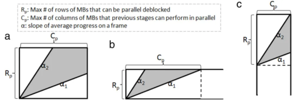
Then,Cp
=
the maximal number of columns of MBs that previous stages can decode in parallel=
Min
MW,
Rpα
1
(8) The maximal number of MBs should be keptin the internal buffer Mbuffered
=
Rp×
Cp−
R2p 2α
2−
α
1×
C 2 p 2 (9)The internal buffer size between these two stages SizeIB
=
Bp×
16×
16×
Mbuffered=
384×
Mbuffered(
bytes).
(10)Though these equations are made for replacing the deblocking stage of the 2D wavefront method with Order4 or Order16, all
equations should be applicable to the internal buffers between any two adjoining video decoding stages. To show realistic numbers, we provideTable 2, which shows the required size of the internal buffer for both Order16and Order4when the frame sizes are 1920
×
Fig. 30. (a) The portion of a frame that has been decoded, (b) the portion of a frame that has been deblocked, and (c) the portion of decoded frame that should be preserved in the internal buffer.
Fig. 31. Portions of decoded frame that should be kept in the internal buffer for different shapes of frames. Table 2
Internal buffer size.
Method Frame size
1920×1080 1080×1920
Order16 1,196,160 305,184
Order4 1,011,200 258,944
Where the size is in number of bytes.
4.5. Memory bandwidth requirements
In this section, we discuss the memory bandwidth require-ments for accessing the internal buffer and the decode picture buffer (DPB). First, the internal buffer shown inFig. 29is used to store the temporal results for the deblocking processes, in which, conventionally, every pixel is read and written four times. Taking a 1920
×
1080 24 fps H.264 coded video as an example, the mem-ory bandwidth requirement for a read or write operation on every pixel could be calculated as follows:Trw
=
Memory bandwidth per read/
write operation on every pixel=
bp×
(
number of pixels in a frame)
×
(
number of frames in one second)
=
1.
5×
1920×
1080×
24=
71.
2 MB/
s.
(11) The memory bandwidth requirement for the internal buffer is characterized by the number of reads and writes occurring in this buffer. When using the internal buffer to store the temporal results, four reads and three writes occur on every pixel in the internal buffer. Consequently, the required memory bandwidth of the inter buffer was determined as follows:Memory bandwidth for reads
=
4×
Trw=
284.
8 MB/
s.
(12) Memory bandwidth for writes=
3×
Trw=
213.
6 MB/
s.
(13)Because only one write (to write the final result) on every pixel occurred in the DPB, the memory bandwidth requirement equaled Trw, which is 71.2 MB/s in this example.
The memory bandwidth requirements for the internal buffer were considerably higher than those of the DPB. This issue could be alleviated dramatically if all the temporal results are bypassed between the PEs. The need for memory access was reduced to only the initial read of each pixel from the internal buffer and the
remaining reads and writes were operated by bypassing between the PEs. Because of the bypassing process, the memory bandwidth requirements are 71.2 MB/s both for reading from the internal buffer and for writing to the DPB.
5. Conclusion
In examining the deblocking algorithm at finer granularity, ad-ditional parallelism can be exploited for speedup or power-saving purposes. To speed up, for 1920
×
1080- and 1080×
1920-pixel frames and given an unlimited number of PEs, our design obtains speedups of 1.92 and 2.44, respectively, compared with the 2D wavefront method, and 1.25 and 1.13, respectively, compared with Order16.Two digital video codec trends are larger frame sizes and better coding compression rates. Hence the role of deblocking will be-come more crucial. Our method can take advantage of more hard-ware resources. In addition, as the frame size grows, our method requires only extra time that is proportional to the square root of the frame size increase when the aspect ratio of frames fixed. These features are very desirable in data-intensive computing.
Above is a significant step towards how speedup and energy ef-ficiency can be achieved in pervasive data-intensive computing for multimedia processing. Two future directions will be attempted: One, whether there are opportunities in other process steps in H.264, and how we can take advantage of these opportunities. And two, if these opportunities and techniques can be extended to run on distributed systems, as many computing resources exist around us in this form.
Acknowledgment
This work is supported in part by the National Science Council of the Republic of China, Taiwan under Grant NSC 98-2221-E-009-073-MY3.
References
[1]X. Liu, L.T. Yang, K. Sohn, High-speed inter-view frame mode decision procedure for multi-view video coding, Future Generation Computer Systems 28 (2012) 947–956.
[2]P. List, A. Joch, J. Lainema, G. Bjontegaard, M. Karczewicz, Adaptive deblocking filter, IEEE Transactions on Circuits and Systems for Video Technology 13 (2003) 614–619.
[7] C. Yen-Kuang, X. Tian, G. Steven, M. Girkar, Towards efficient multi-level threading of H.264 encoder on Intel hyper-threading architectures, in: 18th International Parallel and Distributed Processing Symposium, 2004. Proceedings, 2004, p. 63.
[8] K. Yun-il, K. Jong-Tae, B. Sehyun, B. Hyunki, S. Hyo Jung, H.264/AVC decoder parallelization and optimization on asymetric multicore platform using dynamic load balancing, in: 2008 IEEE International Conference on Multimedia and Expo, 2008, pp. 1001–1004.
[9]M. Hübner, in: J. Becker (Ed.), Multiprocessor System-on-Chip, 2011.
[10]S. Borkar, A.A. Chien, The future of microprocessors, Communications of the ACM 54 (2011) 67–77.
[11] E.B.V.D. Tol, E.G.T. Jaspers, R.H. Gelderblom, Mapping of H.264 decoding on a multiprocessor architecture, 2003, pp. 707–718.
[12]K. Schöffmann, M. Fauster, O. Lampl, L. Böszörmenyi, An evaluation of parallelization concepts for baseline-profile compliant H.264/AVC decoders, in: A.-M. Kermarrec, L. Bougé, T. Priol (Eds.), Euro-Par 2007 Parallel Processing, Springer, Berlin, Heidelberg, 2007, pp. 782–791.
[13]S. Sun, D. Wang, S. Chen, A highly efficient parallel algorithm for H.264 encoder based on macro-block region partition, in: R. Perrott, B. Chapman, J. Subhlok, R. de Mello, L. Yang (Eds.), High Performance Computing and Communications, Springer, Berlin, Heidelberg, 2007, pp. 577–585.
[14] M. Cor, A. Arnaldo, A. Mauricio, J. Ben, R. Alex, Parallel scalability of H.264, 2008.
[15]F.H. Seitner, R.M. Schreier, M. Bleyer, M. Gelautz, Evaluation of data-parallel splitting approaches for H.264 decoding, in: Proceedings of the 6th International Conference on Advances in Mobile Computing and Multimedia, ACM, Linz, Austria, 2008, pp. 40–49.
[16]A. Azevedo, C. Meenderinck, B. Juurlink, A. Terechko, J. Hoogerbrugge, M. Alvarez, A. Ramirez, Parallel H.264 decoding on an embedded multicore processor, in: A. Seznec, J. Emer, M. O’Boyle, M. Martonosi, T. Ungerer (Eds.), High Performance Embedded Architectures and Compilers, Springer, Berlin, Heidelberg, 2009, pp. 404–418.
tures, parallel processing, and embedded system design.
Chung-Ping Chung received the B.E. degree from the Na-tional Cheng-Kung University, Tainan, Taiwan, Republic of China in 1976, and the M.E. and Ph.D. degrees from the Texas A&M University, Texas, USA in 1981 and 1986, respectively, all in Electrical Engineering. He was a lec-turer in electrical engineering at the Texas A&M Univer-sity while working towards the Ph.D. degree. Since 1986 he has been with the Department of Computer Science at the National Chiao Tung University (NCTU), Hsinchu, Tai-wan, ROC, where he is a professor and the associate dean of the College of Computer Science. From 1998, he was on leave from the university and joined the Computer and Communications Laborato-ries, Industrial Technology Research Institute, ROC as the Director of the Advanced Technology Center, and then the Consultant of the General Director’s Office, until 2002. From 2007 to 2011, he was the director of the Institute of Biomedical Engi-neering at NCTU. He also served as the Editor-in-Chief in the Information Engineer-ing Section of the Journal of the Chinese Institute of Engineers (EI, SCI), ROC, in 2000 to 2005, and the editor of the Journal of Information Science and Engineering (SCI) in 2006 to 2012. He has led the Computer Systems Laboratory in the CS department, NCTU since 1992, served as the consultant and reviewer for numerous information and IC companies and government organizations, published over 200 refereed tech-nical papers, and obtained over 20 patents. His research interests include computer architecture, parallel processing, embedded system and SoC design, and paralleliz-ing compilers.