A HEURISTIC ALGORITHM FOR THE RELIABILITY-ORIENTED FILE ASSIGNMENT IN A DISTRIBUTED COMPUTING SYSTEM

(1)

P e r g a m o n

A Heuristic A l g o r i t h m for

t h e Reliability-Oriented File A s s i g n m e n t

in a D i s t r i b u t e d C o m p u t i n g S y s t e m

D . - J . C H E N , W . C . H O L A N D R . - S . C H E N t I n s t i t u t e of Computer Science and Information Engineering

National Chiao Tung University, Hsinchu, Taiwan, R.O.C.

D. T. K.

CHEN

Department of Computer & Information Science Fordham University, Bronx, NY, U.S.A.

(Received and accepted February 1994)

A b s t r a c t - - D i s t r i b u t e d Computing Systems (DCS) have become a major trend in today's computer system design because of their high speed and high reliability. Reliability is an important performance parameter in DCS design. Usually, designers add redundant copies of software and/or hardware to increase the system's reliability. Thus, the distribution of data files can affect the program reliability and system reliability. The reliability-oriented file assignment problem is to find a file distribution such that the program reliability or system reliability is maximized.

In this paper, we develop a heuristic algorithm for the reliability-oriented file assignment problem (HROFA), which uses a careful reduction method to reduce the problem space. Our numerical results indicate that the HROFA algorithm obtains the exact solution in most cases and the compu- tation time is significantly shorter than that needed for an exact method. When HROFA fails to give an exact solution, the derivation from the exact solution is very small.

K e y w o r d s - - F i l e assignment, Distributed computer system (DCS), Memory capacity constraint, Heuristic, Program reliability.

1. I N T R O D U C T I O N

D i s t r i b u t e d c o m p u t i n g s y s t e m s ( D C S ) have b e c o m e i n c r e a s i n g l y p o p u l a r in r e c e n t y e a r s , for t h e a d v e n t o f V L S I t e c h n o l o g y a n d low-cost m i c r o p r o c e s s o r s h a s m a d e d i s t r i b u t e d c o m p u t i n g eco- n o m i c a l l y p r a c t i c a l in t o d a y ' s c o m p u t i n g e n v i r o n m e n t . T h e D C S p r o v i d e s p o t e n t i a l i n c r e a s e s in r e l i a b i l i t y , t h r o u g h p u t , f a u l t t o l e r a n c e , resource s h a r i n g a n d e x t e n d i b i l i t y [1-5]. To i m p r o v e t h e s e p e r f o r m a n c e c h a r a c t e r i s t i c s , we r e q u i r e a careful design of t h e DCS. To i n c r e a s e r e l i a b i l i t y , we c a n a d d r e d u n d a n t c o p i e s o f h a r d w a r e a n d software, such as p r o c e s s i n g e l e m e n t s ( P E ) , p r o g r a m s , a n d d a t a files in different p r o c e s s o r s . T h e d i s t r i b u t i o n of d a t a files c a n affect t h e p r o g r a m r e l i a b i l i t y a n d o v e r a l l r e l i a b i l i t y in t h e DCS. Hence, a n i m p o r t a n t p r o b l e m in D C S d e s i g n is t o find a d a t a file d i s t r i b u t i o n t h a t m a x i m i z e s a c e r t a i n r e l i a b i l i t y m e a s u r e . S e v e r a l n e t w o r k r e l i a b i l i t y m e a s u r e s h a v e b e e n defined a n d a s s o c i a t e d e v a l u a t i o n m e t h o d s h a v e b e e n d e v e l o p e d . T w o of t h e m , D i s t r i b u t e d P r o g r a m R e l i a b i l i t y ( D P R ) [6,7] a n d D i s t r i b u t e d S y s t e m R e l i a b i l i t y ( D S R ) [8-10], a r e a d o p t e d in t h i s p a p e r . F o r a given d i s t r i b u t i o n of p r o g r a m s a n d d a t a files in a D C S , D P R is t h e p r o b a b i l i t y t h a t a given p r o g r a m c a n be r u n s u c c e s s f u l l y a n d will b e a b l e t o access all t h e files it r e q u i r e s from r e m o t e sites in s p i t e of f a u l t s o c c u r r i n g a m o n g tAuthor to whom all correspondence should be addressed.

Typeset by .AA/~-TEX 85

(2)

86 D.-J. CHEN e t al.

the processing elements and communication links. The second measure, DSR, is defined to be the probability t h a t all the programs in the system can be run successfully.

The file assignment problem and related problems such as task assignment and job scheduling have been studied for many years [11-14]. T h e y have been studied by using techniques from graphic theory, queuing theory, mathematical programming, and various heuristic and algorithmic techniques.

The file assignment problem is a special case of the task assignment problem. T h e problem we are concerned with in this paper is to assign files in a DCS so that all the programs are allocated to reading d a t a or outputting data. The file assignment problem is inherently NP-complete [15] in complexity. This implies that optimum solutions can be found only for small problems. For larger problems, it is necessary to introduce heuristics to produce algorithms which generate near-optimum solutions. Several techniques, such as dynamic programming [16], branch-and- bound [17], backtracking [18] and heuristic programming [19], can be used to avoid the complete enumeration of the problem space. The choice of a particular technique depends on the structure of the problem.

T h e reliability-oriented file assignment problem has been studied for many years. In [18], a reliability-oriented file assignment algorithm (ROFA) was proposed to solve the optimal file assignment problem under a memory space constraint. T h a t method first generates all the maximum feasible file combinations (MFFC) of each node, then constructs a space state tree according to each nodes' MFFCs and travels the state space tree in a depth-first manner by applying a back-tracking algorithm.

T h e back-tracking algorithm first finds a feasible solution as a lower bound and then back tracks to level n - 1 of the space state tree. If the reliability upper bound (let the unvisited child nodes contain all required files) is smaller than the lower bound, the downward searching in the space state tree is fathomed. T h e reliability was measured by the SYREL algorithm [20]. Although this method is capable of finding the optimum solution, it is not efficient, so it is probably not a practical approach.

In this paper, we present a heuristic algorithm for the reliability-oriented file assignment problem (HROFA) which uses a careful heuristic pruning method to reduce the solution space. Unlike other assignment strategies, the proposed reduction method is a reasonable one. T h e HROFA algorithm works in a manner similar to that used to find a minimal file spanning tree; the complete algorithm and the justification for our reduction techniques are described in this paper. Numer- ical results show t h a t the HROFA algorithm obtains the exact solution in most cases, and when it fails to give an exact solution, the deviation from the exact solution is quite small.

The organization of the rest of this paper is as follows. In Section 2, the problem statement, notation, and definitions t h a t will be used throughout this paper are given. Section 3 states the reliability oriented file assignment problem in distributed computing systems. T h e derivation, correctness, and some examples of application of the HROFA algorithm are described in Section 4. Section 5 concludes the paper.

2. P R O B L E M S T A T E M E N T , NOTATION,

A N D D E F I N I T I O N S

PaOBLEM STATEMENT. The reliability-oriented file-assignment problem can be characterized as follows:

GIVEN.

Network topology

Distribution of programs in the network Files required by programs for execution T h e size of each file

T h e available memory space of each processing element T h e reliability of each communication link

(3)

A Heuristic A l g o r i t h m 87 C O N S T R A I N T . The limitation of memory space of each processing element

V A R I A B L E . File assignment

GOAL. Maximize D P R of a given program (or Maximize DSR of the system)

N O T A T I O N A N D D E F I N I T I O N S . c(v, E) N~ P R G F~ P R G p D P R p F~ F ~ F S T M F S T A n u n d i r e c t e d g r a p h in w h i c h V M F F C r e p r e s e n t s t h e n o d e set of processing e l e m e n t s a n d E r e p r e s e n t s t h e e d g e s e t of c o m m u n i c a t i o n links for t h e n e t w o r k u n d e r c o n s i d e r a t i o n n a n o d e i in V k t h e set of p r o g r a m s a l l o c a t e d in t h e n e t w o r k for e x e c u t i o n P(q) t h e set of files r e q u i r e d by P R G

Ip

a p r o g r a m p in P R G 8i t h e reliability of d i s t r i b u t e d c~ p r o g r a m p t h e file i in Fs xi,j

t h e set o f files required by P R G p

for e x e c u t i o n X}t)

a s p a n n i n g t r e e t h a t c o n n e c t s t h e r o o t n o d e ( p r o c e s s i n g e l e m e n t s

t h a t r u n s t h e p r o g r a m u n d e r FAr c o n s i d e r a t i o n ) to o t h e r n o d e s s u c h E ( P R G p ) t h a t its vertices hold all t h e n e e d e d

files a n F S T s u c h t h a t t h e r e e x i s t s no o t h e r F S T w h i c h is a s u b s e t of it P r ( E ) P(i, k) a feasible file c o m b i n a t i o n s u c h t h a t t h e r e e x i s t s no o t h e r feasible file c o m b i n a t i o n w h i c h is a s u p e r s e t of it t h e n u m b e r of n o d e s in G; n -- IVI t h e n u m b e r s of files in Fs t h e p r o b a b i l i t y t h a t t h e c o m m u n i - c a t i o n link w o r k s (fails) t h e i n d e x s e t of FNp t h e size of Fi t h e available m e m o r y s p a c e of N~ t h e i n d i c a t o r of file a s s i g n m e n t x~,j = 1 if Fj is a s s i g n e d to N i , else 0

a feasible file c o m b i n a t i o n of Ni; ~ , il i2 ' ' ' ~ a set of M F F C s for N i e v e n t t h a t P R G p c a n s u c c e s s f u l l y r u n a n d files in FNp c a n b e s u c c e s s f u l l y accessed by P R G p p r o b a b i l i t y of e v e n t E a t w o - d i m e n s i o n a l a r r a y s u c h t h a t if t h e r e is a s o l u t i o n t o t h e file c o m b i n a t i o n p r o b l e m w i t h t h e first i e l e m e n t s a n d size k

3. T H E R E L I A B I L I T Y - O R I E N T E D

F I L E A S S I G N M E N T

P R O B L E M I N D I S T R I B U T E D

C O M P U T I N G

S Y S T E M

We shall now formally define the reliability-oriented file assignment problem. The reliability oriented file assignment problem can be stated mathematically as follows:

PROBLEM 1.

(Maximizing

D P R

subject to memory

space

constraint)

Maximize DPRp = Pr [E (PRGB)] k

{

~ sjx/j < C~, j = l subject to ~ X~j > 1, 4=1 x~j = 0 o r 1, i = l . . . . ,n. i = 1 , 2 , . . . , n .

(4)

88 D.-J. CHEN et al.

PROBLEM 2. (Maximizing D S R subject to m e m o r y space constraint)

Maximize DSR = Pr [i=Q E (PRG~) ] j = l subject to X~j _> 1, i=1 x i j = O o r 1, i = l , . . . , n , j = 1 , 2 , . . . , k . i = 1 , 2 , . . . , n . j = 1 , 2 , . . . , k .

First, we present a back-tracking algorithm [18] for solving Problem 1. The algorithm has two steps:

(1) For each node Ni, find all of the maximal feasible file combinations (MFFC). (2) Apply a back-tracking algorithm to find the optimal file assignment.

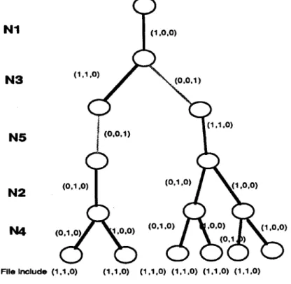
The following numerical example illustrates the operation of the back-tracking algorithm. Consider the distributed processing system shown in Figure 1, which consists of six nodes and the PRG1.

"s

P1 needs F1, F2, F3

File size: 2, 3, 5

Node capacity: 2, 3, 5, 4, 5, 2

for NI,N2,N3,N4.N5 and N6

respectively

Edge reliability: 0.9

File Combinations:

FAI= { (1,0,0) }

FA2= { (0,1,0), (1,0,0))

FA3= ((1,1,0), (0,0,1))

FA4= { (0,1,0), (1,0,0) }

FAS= ( (1,1,0), (0,0,1) }

FA6= ( (1,0,0) }

Figure 1. A simple DCS for illustration of the back-tracking algorithm.

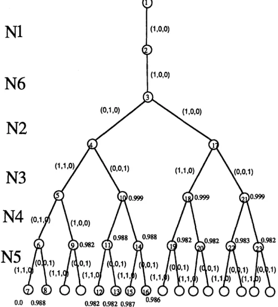
Two copies of program PRG1 are allocated in node N1 and N6, respectively. The files required for executing program PRG1 are F1, F2, and F3. The file sizes of F1, F2, and F3 are 2, 3, and 5. Assume that all the communication links have the same reliability, 0.9. The available memory space for N1 to N 6 i s M1 = 2, M2 = 3, M3 = 5, M4 = 4, M5 = 5, and M6 = 2. In Step 1, we generate all MFFCs for each node. These are F A 1 = {(1, 0, 0)}, F A 2 = {(0, 1,0), (1, 0, 0)},

F A 3 = {(1,1,0), (0,0,1)}, F A 4 = {(0,1,0), (1,0,0)}, F A 5 = {(1,1,0), (0,0,1)}, and F A 6 =

{(1,0,0)}. The nodes in Figure 2 have been numbered according to the sequence of the back- tracking procedure. The bounding function is applied at number 9 of the state space tree. The reliability upper bound 0.982 is less than the lower bound 0.988 found so far, so then node 9 is fathomed. The more precise upper bound will be estimated at the lower level of the state space tree. The optimal solution is [(xn, X12, X13), (X21, 3g22, X23), (X31, X32, X33), (X41, X42, X43), (Xsl,X52,Z53), (X61,X62, Z63)] = [(1,0,0), (0, 1,0), (1, 1,0), (0, 1,0), (0,0, 1), (1,0,0)]. The opti- mal value of DPR1 is equal to 0.988.

The back-tracking process is an elegant method. In real cases, however, the reliability difference between all feasible solutions is not so clear. A small reliability difference is easily obtained by the reliability contribution of the Fullfile nodes (the unvisited nodes) which are assumed in the back-tracking algorithm. The more Fullfile nodes a state assumes, the higher its reliability. So

(5)

N1

N6

A Heuristic Algorithm

¢)

(1 ,o,o)

89

N2

(O,l,O) 7

~

(1,o,o)

N3

N4

(0,1

N5

(1,1 ,o)

(1 ,o,o)

!o,o,1)

(1,1,o) /

\,(o,o,1)

)0.999 ~'~10.999 ~ 0 . 9 9 9

0.988

(1,1;¢~ t <i,i,<~ +X 'i, ,4 "X ;,'., ,(,'V;:., I,''~'.'! I t~,+,:,?, l!o,~,?>, l(O,V,)

0.0 0.988 0.982 0.982 0.987 0.986

Figure 2. Generation of the state space tree for Figure 1.

the pruning will rarely occur in the high levels of the state space tree; most of the pruning will occur in the last few levels of the state space tree (because there are fewer Fullfile nodes in t h a t pathset). Hence, this m e t h o d m a y take more time t h a n an exhaustive search. T h e example shown in Figure 2 provides the evidence for this conclusion (there are only 16 pathsets, but the back-tracking algorithm travels 23 states). So the branch-and-bound method is not well suited for the ROFA problem.

Also, the connection of a network has an i m p o r t a n t influence on the certain reliability. This fact motivates us to develop a heuristic algorithm, which we call HROFA, t h a t uses information on network connections and analyzes D P R formulas to avoid exhaustive enumeration of the state space tree.

4. D E R I V A T I O N OF T H E H R O F A A L G O R I T H M

Nair [12] proposed a heuristic method for choosing the p a t h s e t with the highest possible reliability (under some assignment). Let the p a t h be assigned according to this method. T h e n choose the p a t h s e t with the next highest reliability and assign the p a t h to it, and so on. T h e m a x i m a l error rate of this m e t h o d is under 4.8%, and in most cases, it successfully derives the correct answer.

(6)

90 D.-J. CHEN et al.

We can s t a r t spanning our state space tree by constructing the most reliable MFST. T h a t is, spanning the state space tree is just like finding its MFST. Using this basic idea for analyzing the D P R formula, we propose a heuristic algorithm for the reliability oriented file assignment problem. We call the algorithm HROFA (Heuristic algorithm for ROFA).

4.1. T h e P r o p o s e d H e u r i s t i c A l g o r i t h m ( H R O F A )

In the H R O F A algorithm, we span the state space tree like ROFA does. We reduce the s t a t e space tree in a top-down manner by checking its file combination, and the nodes are spanned in different order. T h e following is an outline of HROFA:

(1) G e n e r a t e the spanning order of each node. (2) Perform H R O F A algorithm to span the state tree. STEP 1.

(a) Calculate the spanning order of each node.

T h e order is measured by the node reliable degree (RD). RDi = Xs# * Ff~n/~

where X,,i is the average link reliability from Node i to Node s (the starting nodes). F/nn A is the average number of needed files contained in Node i.

Example: If the M F F C s of Ni are (1,1,0), (0,0,1) and the file needed is (1,1,1), t h e n Finny ` = (2 + 1)/2 = 3/2.

T h e X , # = 0.9 (suppose the reliability of all links is 0.9), and RDi = 0.9 • 3/2 = 1.35. (b) Find the node t h a t has the highest RD and add this node to StartNode. R e p e a t the

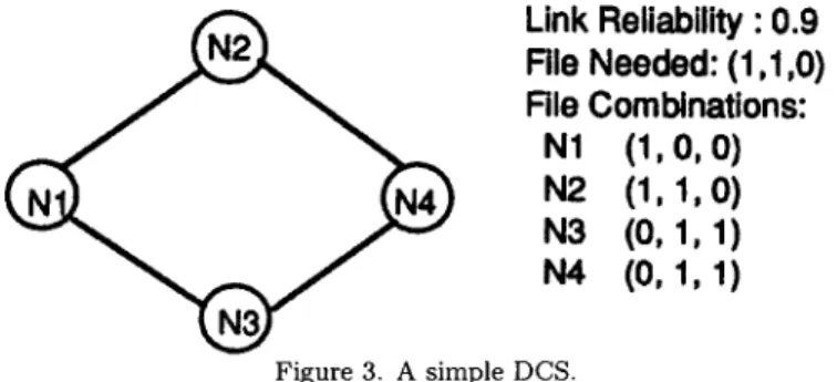
process until the spanning order of all nodes is found. For example, consider the network below:

Link Reliability : 0.9

File Needed: (1,1,0)

Rle Combinations:

N1 (1,0, 0)

N2 (1, 1,0)

N3 (0,1,1)

N4 (0, 1, 1)

Figure 3. A simple DCS.

Since the link reliability is 0.9, the Xs,i for each node is 0.9, and the F/,,nl, for each node is {1,2,1,1}.

Table 1. The generation of spanning order for Figure 3.

StartNode 1 2 3 4

1 - 0.9*2 0.9.1 -

1,2 - - 0.9.1 0.9.1

1, 2, 3 - - - 0.9 * 1

1, 2, 3, 4 . . . .

So the spanning order is N1, N2, N3, N4. Let the node sequence be Nil, Ni2, N~3 . . . . N~n, and span the state space tree in t h a t sequence. Spanning to some node, if we find paths t h a t contain all the needed files, then we delete their brother paths which do not contain all the needed files, i.e., we mask the Fg.n. We then continue spanning, and if we find pathsets t h a t can be reduced,

t h e n we mask FN~2. We repeat the above reduction method until no pathset can be reduced or

(7)

A Heuristic Algorithm 91

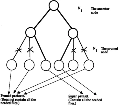
ancestor

The pruned node

l~ul

(Does not contain all the (Contain all the needed

needed files.) files.)

Figure 4. T h e pruned pathsets and the super pathsets.

4.2. A l g o r i t h m

Now we present a heuristic algorithm for computing the ROFA problem under m e m o r y space constraints. This is an enumerative algorithm which uses heuristic reduction to reduce the state space tree. T h e algorithm consists of four steps, as follows:

Step 0. Step 1. Step 2. Step 3. Step 4. Initialization.

Generate all MFFCs of all nodes.

Generate the spanning order of each node.

Span the state space tree by the spanning order and perform heuristic reduction. Compute the reliability of each pathset spanned in Step 3 and o u t p u t the best file assignment.

S t e p 0. I n i t i a l i z a t i o n

We read the d a t a from the file which contains the system parameters to obtaining the following information: N = number of nodes L -- number of links F = number of files P = number of programs C ( i ) = capacity of node i S ( i ) = size of file i

P N ( i ) = file needed for program i to be executed

S t e p 1. G e n e r a t e all M F F C s o f all n o d e s

We solve this problem using a dynamic programming technique. Since the problem constraints are

(8)

92 D.-J. CHEN et al.

XIS(1) + X2S(2) +... + X F S ( F ) <_ C(i),

where

Zj

= 1, if file j is contained in node, else 0.

It can be divided into several subproblems as follows:

x,s(1) + x s(2) +... + X S(F) = C(i)

XIS(1) + X2S(2) +... + X F S ( F ) = C(i) - 1

X1S(1) + X2S(2) + . . . + X F S ( F ) = C(i)-MaxFileSize.

Each of these problems is just the Knapsack problem and the feasible solution is a file assignment of it.

(C(i)-MaxFileSize) is set as a bound because, if there exists an M F F C in which X1S(1) + X2S(2) + . . . + X F S ( F ) < C(i)-MaxFileSize,

then we can add another file not included in this M F F C and the total file size will still be smaller t h a n N ( i ) , which is a contradiction. So there is no M F F C with total size smaller t h a n (C(i)-MaxFileSize).

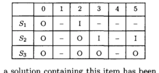
We use a dynamic p r o g r a m m i n g technique to generate a table which indicates if there exists a solution in the size of (see Table 2).

Table 2. Table generated by Knapsack algorithm.

0 $1 o $2 o s3 o 1 2 3 4 5 - I - - - - 0 I - I - 0 0 - 0

T : a solution containing this item has been found

'O': a solution without this item has been found

' - " no solution of this size T

If there is a solution in the entry P(i, k), then we will check whether P(i - 1, k - Si) has a

solution in it. If so, we continue checking until we check P(0, 0). When we find a feasible file combination, we will check whether it is covered by or covers the F F C s found before. We t h e n delete the F F C if it is covered by other FFCs, or add the F F C to FOUND, if it is not covered. T h e following is a formal description of Step h

M F F C ( K ) .

/ * S ( t h e array t h a t stores the file size). K , the node capacity, P (a two-dimensional array such t h a t p[i, k]E = true if there exists a solution to the file combination problem with the first i elements and size k, and P[i, k]B -- true if the ith element belongs to t h a t solution*/

begin if ~ S[i] < K t h e n begin M F F C = (1, 1, 1 . . . . ) r e t u r n end K n a p s a c k ( K ) F F C = 0

(9)

A Heuristic Algorithm 93 f o r t ---- K downto K-MaxFileSize do check(K, t, FFC) e n d

function

Knapsack(K) begin P[0, 0]E -- true f o r k = l t o K do P[0,

k]E =

false f o r i : l t o F do f o r k = 0 t o K do

P[i, k]E =

false if

P [ i - 1 , k ] E

then begin

P[i, k]E

= true

P[i, k]B

= false end

e l s e i f

k - S[i] >_0

then

i f

P[i - 1, k - S[i]]E

then begin

P[i, k]E

= true

P[i, k]B

= true end od end

function

C H E C K ( K , t, FFC) b e g i n if K -- 0 then

check if F F C is covered or covers other elements in F O U N D , add to F O U N D if the F F C is not covered

f o r i = t to N do if

P[t,K]E

t h e n b e g i n FFC[ = 1 << i c h e c k ( g -

S[t],

t - 1, FFC) end e l s e i f

K - S I t ] >_0

t h e n begin F F C I = I << i check(K - S[t]), t, FFC) e n d e n d od S t e p 2. G e n e r a t e t h e s p a n n i n g o r d e r o f e a c h n o d e

In Step 2, we choose a starting node which contains the program to be executed and add t h a t starting node to StaxtNode(0). We then compute the Reliable degree (RD) of each node to the StartNode and choose the most reliable node to add to StartNode(1). According to the new StartNode, we find the most reliable node from among the rest of the nodes and add it to StartNode(2). We repeat the process until all nodes have been added to StartNode. The StartNode records the spanning order of each node.

(10)

S t e p 3. Perform HROFA algorithm

T h e HROFA algorithm acts as follows: According to the spanning order, we span the state space tree in DFS manner. While spanning to a node, if we find there exist pathsets which contain all the needed files, we eliminate the other pathsets t h a t do not contain all the needed files. T h e n we mask the MFFCs of the node which is in StartNode(1) and continue spanning to other nodes not yet spanned. If we find there exist pathsets that contain all the needed files, we cut the other pathsets which do not contain all the needed files. We then mask the MFFCs in StartNode(2), and continue the spanning and cutting process described above. We repeat the process until all MFFCs of each node have been spanned. The formal HROFA algorithm is given below.

H R O F A (SPANNODE, MASKNODE, PATHSET).

/* The SpanNode is the node to be spanned. The MaskNode is the node whose MFFCs are masked * /

begin

i f SpanNode = 0 t h e n b e g i n

add the Pathset to FOUND r e t u r n

end

f o r all the MFFCs of the SpanNode do

i f the file included in the pathset contains all the needed files t h e n begin

temp = Pathset I the MFFC

HROFA(the next node of the SpanNode, the next node of the MaskNode, temp) end

od

i f there does not exist a pathset which contains all the needed files t h e n begin

f o r all MFFC in SpanNode do

temp = Pathset I the MFFC

HROFA(the next node of SpanNode, MaskNode, temp) od

end end

Step 4. C o m p u t e the r e l i a b i l i t y o f e a c h pathset

Since the system parameters have been read in Step 0, we know the network topology, the program distribution, the files needed for each program to be executed, and the link reliability. We still need to know the file distribution of each node in order to compute the pathset reliability. In this step, we simply pass the file distribution of each node according to the pathset in the FOUND. T h e n we call the reliability evaluating program F R E A [21] to compute the pathset reliability. After computing all the reliabilities, we will o u t p u t the file assignment with the highest reliability.

T h e complete algorithm

(11)

A H e u r i s t i c A l g o r i t h m 95 H R O F A ALGORITHM. S T E P 0 . I n i t i a l i z a t i o n . read system p a r a m e t e r s F O U N D =

F N =

(.J Fj

S T E P S T E P S T E P S T E P Pj EPN

find a node xi in the DCS t h a t contains the p r o g r a m to be executed S t a r t N o d e = xi

MaskNode = 0

1. G e n e r a t e M F F C s of all nodes. f o r all nodes do

M F F C ( n o d e capacity)

2. G e n e r a t e the spanning order of each node. N e x t N o d e ( S t a r t N o d e ) 3. Perform H R O F A algorithm. p a t h s e t -- 0 H R O F A ( S t a r t N o d e , MaskNode, pathset) 4. C o m p u t e p a t h s e t reliability. f o r each p a t h s e t in F O U N D do

call F R E A to evaluate the pathset reliability o u t p u t the assignment which has the highest reliability

4.3. Examples

We use the DCS shown in Figure 1 as an example to show how the HROFA works. STEP 0. Initialization.

T h e system p a r a m e t e r s are known. T h e node capacity for node 1 to node 6 is 2,3,5,4,5,2. T h e file sizes for F1 to F3 are 2, 3, and 5. All the link reliabilities are the same and equal 0.9. T w o copies of p r o g r a m PRG1 are allocated in node 1 and node 6. T h e files needed for PRG1 are F1, F2, and F3.

STEP 1. G e n e r a t e the M F F C s of each node. T h e K n a p s a c k generates a table as follows:

T a b l e 3. T a b l e g e n e r a t e d for t h e e x a m p l e . NodeSize FileSize $1 82 83 0 1 2 3 4 5 O - I - - 0 - 0 I - I 0 0 0 - 0 Node[l]. M F F C = {(1,0,0)} Node[2 I. M F F C = {(0,1,0),(1,0,0)} Node[3]. M F F C = {(1,1,0),(0,0,1)} Node[4]. M F F C = {(0,1,0),(1,0,0)} Node[5]. M F F C = {(1,1,0),(0,0,1)} Node[6]. M F F C = {(1,0,0)}

(12)

96 D.-J. CHEN et al. S T E P 2 . G e n e r a t e t h e s p a n n i n g o r d e r o f e a c h n o d e . T a b l e 4. T a b l e g e n e r a t e d for t h e e x a m p l e in S t e p 2. S t a r t N o d e S e t R D 1 R D 2 1 - 0.9 1,3 - 0.9 1,3,5 - 0.9 1,3,5,2 - - 1,3,5,2,4 - - 1,3,5,2,4,6 R D 3 R D 4 R D 5 R D 6 1.35 0 0 0 - 0 1 . 3 5 0 - 0 . 9 - 0 . 9 - 0 . 9 - 0.9 - - - 0.9

The spanning order is {1, 3, 5, 2, 4, 6}. STEP 3. Perform heuristic reduction.

N1

~

( 1 , 0 , 0 )

N1

~(1,0,0)

N3 (1'1'~

0'1)

(a) S p a n N o d e = N1, M a s k N o d e = 0. (b) S p a n N o d e = N3, M a s k N o d e = 0. F i g u r e 5. T h e r e s u l t in H R O F A S t e p 3a. RIo Include

N1

(~)(.~,o,o)

N3

o,~,o1~1

(1,1,0) (1,1,1) (1,1,1) (1,0,1) (c) S p a n N o d e = N5, M a s k N o d e = O.

N1

N3

N5

N2

R ] o L ~ l e F i g u r e 6. T h e r e s u l t in H R O F A S t e p 3b.

(

J

(1,1,1)

()

(1 ,o,o)

(

/

(o,o,1) o)

,o) (o,l,o)

/ \

(1,0,1) 11,1,0) 11,1,0) (d) S p a n N o d e = N2, M a s k N o d e = N3. F i g u r e 7. T h e r e s u l t in H R O F A S t e p 3c. F i g u r e 8. T h e r e s u l t in H R O F A S t e p 3d.

(13)

N 1 N 3 A Heuristic Algorithm

%

(1.1,0) £ . u , u )

| I1.1 .o)

N 5

()(°'°'1)

N 2 (o,1 ,o) (o,1 o,.) j~

~,o,o)

Q

i ~ - ~

N4 (o~~,....,)

~,) (o.1.~ ~.~~.. )

File

Include (1,1.O)

(1,1,O) (1,1,0) (1,1,0) (1,1,0) (1,1,0)

(e) SpanNode = N4, MaskNode = N3, N5. Figure 9. The result in HROFA Step 3e.

97

N1

I

(1,0.0)

N3

N5

(0,0.1)

(1,1,0)

N2 I (0.1,0) (0,1,0)

N4

(O.l.O)

/ ~1~1,o,o) (O,l,O) / ~(1,o.o)

N6

(1 ,o.o)

~

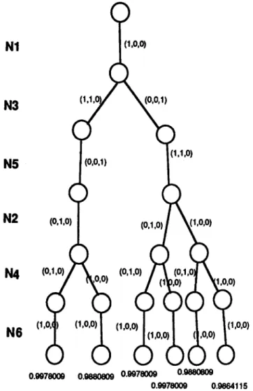
0) (f) SpanNode = N6, MaskNode = N3, N5.

Figure 10. The result after HROFA Step 3. STEP 4. C o m p u t e t h e p a t h s e t reliability.

T h e best assignments for N1, N2, N3, N4, N5, N6 are {(1,0,0), (0,1,0), (1,1,0), (0,1,0), (0,0,1), (1,0,0)} (see Figure 11).

(14)

98

N1

N3

N5

N2

N4

N6

D.-J. CHEN et al.

©

~

~,(0,0,1)

~,1,0)

()

(

10,1,0) 10,1,01

,,,;

.o.,

0.gg7800g 0.g88080g 0.gg7800g o.gg7eoog

Figure 11. The result in HROFA Step 4.

pathget A B

~ ~I,0,0)

i ,0) (~,0,0)

o.g880eog 0.g664115 NI C

Figure 12. Example showing correspouding pathsets.

4 . 4 . T h e C o r r e c t n e s s o f t h e H R O F A A l g o r i t h m

To perform the pruning described above, the reliability of each pathset of the pruned subtree must be less than or equal to the corresponding super pathsets.

W h a t are the corresponding pathsets? Consider Figure 12.

Pathsets A, B, and C are corresponding pathsets, i.e., these pathsets differ in only one MFFC, which is on the pruned level (node Nj). This means all these file assignments of the corresponding pathsets are different in only one node and that node is on the level where pruning occurred.

(15)

A Heuristic Algorithm

Figure 13. pathsets.

(1,0,1)

Example showing the different file assignments between corresponding

(~~,~)

(~)

(~,o,~)

reduceto

- (1,1,0) N ~

(l, o, 1)

Figure 14. Example showing different file assignments between corresponding pathsets.

99

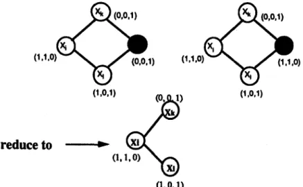
In Figure 13, the two networks are different in the file-assignment of

Nj.

Since there is only

one node difference, we divide all the M F S T s of a pathset into three cases. We t h e n observe the following facts:

CASE 1. T h e M F S T does not include the pruned node, and the reliability of the corresponding p a t h s e t s is the same.

We can regard the network as if it were reduced to a subgraph (Figure 14). T h e M F S T s of the corresponding pathsets are generated from the same file assignment, and the pathsets have the same MFSTs. If we span the M F S T s ' probability in the same p a t h order, the same M F S T should have the same probability. So the total reliability of the M F S T s which do not include the pruned node is the same. We denote the reliability difference between the super p a t h s e t and the pruned p a t h s e t in Case 1 by D1.

CASE 2. T h e M F S T contains the pruned node. We divided the problem into two parts.

CASE 2A. T h e M F S T contains all the ancestor nodes. T h e reliability of the Super p a t h s e t is superior.

Since it spans the state space tree from the start node to all of the ancestor nodes and the pruned node, the super pathset already has all the needed files, but the pruned p a t h s e t must connect to other nodes so as to contain all the needed files. So the probability of the M F S T s of a pruned p a t h s e t must be smaller t h a n t h a t of the super pathset. For example, from the file assignment of the super pathset, one can generate as M F S T like t h a t shown in Figure 15.

As shown in Figure 16, however, the pruned pathset should have more nodes to generate an MFST. Even if the pruned pathset has more MFSTs, its total probability is still smaller t h a n t h a t of the super pathset. No m a t t e r how m a n y M F S T s the pruned pathset has (even if it has

(16)

Figure 15. An MFST of the super pathset.

Figure 16. Possible MFSTs of the pruned pathset.

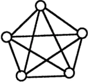
Figure 17. A five-node fully connected network. infinitely m a n y MFSTs), the total probability is

0.93 + 0.1 * 0.93 -~ 0.12 * 0.93 -t- . . . . 0.92(0.9 + 0.09 + 0.009 + - .. ),

which is still smaller t h a n the 0.92 of the super pathset (by measuring Figure 16 and Figure 17 and supposing the reliability of all links is 0.9).

We let the reliability difference between the corresponding pathsets in Case 2a be Da.

CASE 2B. At least one ancestor node is not included in the MFST. T h e reliability difference between the p a t h s e t is small.

T h e probability of Case 2b is given by a t e r m of the form HqiHpj. Because each M F S T in Case 2b probability derivation is multiplied by more t h a n one t e r m q, the reliability difference between the super pathset and the pruned pathset in Case 2b is very small. Let the difference

between the corresponding pathsets be Db.

Today, link reliability of more t h a n 0.9 is quite common, and the t e r m q is typically smaller t h a n 0.1. Since the probability of each M F S T in Case 2b is multiplied by more t h a n one such q, Case 2b contributes less to the probability t h a n Case 2a does. We cannot say the total reliability contribution of Case 2b must be smaller t h a n t h a t of Case 1, for there m a y be m a n y variations in the network topology, file distribution, and program distribution in a DCS, so there could be exceptions. However, we can say t h a t in most cases the total probability contribution is a p p r o x i m a t e l y equal to Case 2b and is about 5% of a system's reliability. So Db is typically quite small.

T h e worst case for our reduction could be t h a t the super pathsets of Case 2b have no M F S T and the pruned pathsets have m a n y MFSTs. Even in this case, however, the error rate is still quite small (because Da reduce the error, and Db is inherently very small, a b o u t 5% of system reliability).

T h e restriction of Case 1 is t h a t one node (the done node) is not included, but in Case 2b, at least one ancestor node is not included and this node is connected to the pruned node. This means t h a t in Case 2b, the DCS is reduced to a subgraph t h a t is smaller t h a n t h a t of Case 1. Each condition in Case 2b is likely to have fewer M F S T s t h a n Case 1, and the probability of

(17)

A Heuristic Algorithm 101 their M F S T s is multiplied by more q's. If the link reliability is 0.9, ten similar M F S T s may be needed to save a q term. In Case 1, the M F S T ' s probability expression could be 0.12 • 0.93, but in Case 2b, it is 0.13 • 0.93. So ten such MFSTs may be needed. In other words, the reduction process is just like

D P R

=pi + q , p j +q2 ,pk + . . . +

qZ, (pi + q , p j + q 2 , p k + . . . ) +

qm, (...)+

HROFA (no mask node) HROFA (mask StartNode[1]) HROFA (mask StartNode[2]), w h e r e l < m < n . . . .

We cut the pathsets which are less reliable in each span level. In HROFA (no mask node), we cut the pathsets which have the smaller product for the term (pi + q • / P + q2 , pk + . . . +). In HROFA, (mask StartNode[1]), we cut the pathsets which have the same value for term 1

(pi + q, pj + q2, pk + . . . ),

but have a smaller value for term 2

(ql , (pi + q , pj + q2, pk +...)).

T h e HROFA (mask StartNode[2]) cuts the pathsets which have the same value for term 1 and t e r m 2 but a smaller value for term 3, and so on. If an exception occurs, it must be t h a t the

Da

is quite small and the pruned pathset has many more MFSTs than the super pathset in Case 2b. Such a condition will occur in a fully connected network.

In a fully connected network, there are many MFSTs in each possible file assignment for a certain program. Thus, when we execute the HROFA algorithm, the reliability difference between the corresponding pathsets in Case 2a will be very small. T h a t is, D~ will probably be reduced to be a value like 0.0000081, or else

Da

will no longer be a great advantage to

Db,

for the pruned pathset would probably have many more MFSTs than the super pathset in such a topology.

In such a topology, the most important parameter influencing the reliability is the load balanced. Because there are many paths that connect two different nodes, under the limitation of m e m o r y space constraints, the more load-balanced the network is, the more choices there are for a program to access the needed files, and thus the more MFSTs exist.

To sum up, our method is to reduce the pathsets whose reliability in Case 1 (about 90% of system reliability) is smaller than that of the other super pathsets, and thus for which the difference D~ is bigger than Db. It is highly unlikely that the reliability of the reduced pathset will be greater than t h a t of the super pathsets. This is the main justification for this reduction method.

4.5. S o m e N u m e r i c a l Results

We now compare the reliability given by the HROFA algorithm with the optimal reliability obtained by complete enumeration. For a given network topology, we compare the difference between the optimal solution for the reliability and the reliability obtained by the HROFA algorithm under variations in the program distribution and link reliability.

EXAMPLE 1. Figure 18. A P1 ne~ls F1, F2, F3,F4 " ~ File size: 2, 3, 4, 5 Node capacity: 4, 5, 7 , 6 . 7 , 4

(18)

Table 5. The numerical result for Example 1.

P1 in 1 (1,2) (1,3) (1,4) (1,5) (1,6) p - - 0 . 9 reliability 0.0000000 0.0000000 0.0000000 0.0000000 0.0000000 0.0000000 difference p = 0 . 8 reliability 0.0000000 0.0000000 0.0000000 0.0000000 0.0000000 0.0000000 difference p----0.7 reliability difference O P T reliability p - - 0 . 9 p = 0 . 8 p = 0 . 7 0.0000000 0.9882000 0.9472000 0.8722000 0.0000000 0.9987948 0.9887744 0.9575776 0.0000000 0.9988119 0.9892352 0.9604693 0.0000000 0.9999118 0.9975398 0.9839450 0.0000000 0.9999579 0.9987379 0.9820002 0.0000000 0.9998462 0.9968845 0.9820002 Total pathsets: 1296 After HROFA: 108 E X A M P L E 2. P1 need F1, F2 ,F3 Node capacity: 2 3 5 4 5 2 File Size: 2 3 5 Figure 19. A six node fully connected network topology.

Table 6. The result for Example 2.

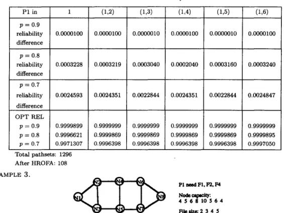
P1 in 1 (1,2) (1,3) (1,4) (1,5) (1,6) p = 0 . 9 reliability difference p = 0 . 8 reliability difference p = 0 . 7 reliability difference O P T REL p = 0 . 9 p - - 0 . 8 p = 0 . 7 0.0000100 0.0003228 0.0024593 0.9999899 0.9996621 0.9971307 Total pathsets: 1296 After HROFA: 108 0.0000100 0.0003219 0.0024351 0.9999999 0.9999869 0.9996398 0.0000010 0.0003040 0.0022844 0.9999999 0.9999869 0.9996398 0.0000100 0.0002040 0.0024351 0.9999999 0.9999869 0.9996398 0.0000010 0.0003160 0.0022844 0.9999999 0.9999869 0.9996398 E X A M P L E 3. 0.0000100 0.0003240 0.0024847 0.9999999 0.9999895 0.9997050 PI need FI, F2. F4 Node ~ t y : 4 5 6 8 1 0 5 6 4 Fileslze: 2 3 4 5

(19)

A Heuristic Algorithm Table 7. The result for Example 3.

103 P1 in (1,2) (1,3) (1,4) (1,5) (1,6) (1,7) (1,8) p--0.9 reliability 0.0000000 0.0000000 0.0000000 0.0000000 0.0000000 0.0000000 0.0000000 difference p = 0 . 8 reliability 0.0000000 0.0000000 0.0000000 0.0000000 0.0000000 0.0000000 0.0000000 difference p = 0 . 7 reliability 0.0000000 0.0000000 0.0000000 0.0000000 0.0000000 0.0000000 0.0000000 difference OPT REL p----0.9 p--0.8 p--0.7

The number of total pathsets: 10935 0.9989100 0.9972122 0.9836672 After HROFA: 3329 0.9989100 0.9907200 0.9673300 0.99989100 0.99072000 0.96733000 0.9999999 0.9999999 0.9941340 0.9999776 0.9992397 0.9941340 0.9999776 0.9995397 0.9941340 0.9998608 0.9972122 0.9836672s

W h e n we a p p l y the HROFA algorithm, an exception will occur when the network topology is fully connected. This is because the superior reliability p a r t (Case 2a contains the pruned node and all of the ancestor nodes) for Super pathsets becomes very small, and the reliability difference from Case 2b (containing the pruned node and at least one ancestor node not included) becomes significant for the m a n y M F S T s in it. Even so, the deviation is no more t h a n 0.25% (at a link reliability of 0.7).

5. C O N C L U S I O N

Distributed C o m p u t i n g Systems (DCS) have become a m a j o r trend in t o d a y ' s c o m p u t e r sys- t e m design for their high fault-tolerance, potential for parallel processing, and b e t t e r reliability performance. One i m p o r t a n t characteristic of a DCS is t h a t it offers redundant copies of software a n d / o r hardware to improve the reliability of the system. One i m p o r t a n t problem in DCS design is the file assignment problem. This problem has been proved to be an N P - c o m p l e t e problem. Traditional solution techniques such as the back-tracking algorithm and m a t h e m a t i - cal p r o g r a m m i n g can give the optimal solution, but they cannot effectively reduce the problem space. Sometimes, an application requires a fast way to compute reliability because of resource considerations. In this situation, deriving the optimal reliability m a y not be a wise idea. Instead, a fast m e t h o d yielding near optimal reliability is preferable.

In this paper, we develop a heuristic algorithm (HROFA) for the reliability-oriented file assignment problem t h a t uses a careful reduction method to reduce the problem space. Our numeral results show t h a t the H R O F A algorithm obtains the exact solution in most case and the compu- tation t i m e is significantly shorter t h a n t h a t needed for an exact method. W h e n H R O F A fails to give an exact solution, the deviation from the exact solution is very small.

R E F E R E N C E S

1. D.P. Agrawal, Advanced Computer Architecture, 376 pages, Computer Society of the IEEE, (1988). 2. T.C.K. Chou and J.A. Abraham, Load redistribution under failure in distributed systems, I E E E Trans.

Comput. 32, 799-808 (1983).

3. D.W. Davies et al., Distributed systems architecture and implementation, Lecture Notes in Computer Science, p. 105, Springer-Verlag, Berlin, Germany, (1981).

(20)

104 D.-J. CHEN et al.

5. J. Garcia-Molina, Reliability issues for fully replicated distributed database, I E E E Computer 16, 34-42 (1982).

6. V.K. Prasnna Kumax, S. Hariri and C.S. Raghavendra, Distributed program reliability analysis, I E E E

Trans. Software Eng. 12 (I), 42-50 (1986).

7. A. Kumar, S. Rai and D.P. Agrawai, On computer communication network reliability under program execution constraints, I E E E Journal on Selevted Areas in Communication 6 (8), 1393-1399 (1988). 8. S. Hariri, C.S. Raghavendra and V.K. Kumar, Reliability analysis in distributed systems, In I E E E '86

Distributed System Conf., pp. 564-571, (1986).

9. V.K. Kumar, S. Hariri and C.S. Raghavendra, Distributed program reliability analysis, I E E E Trans. Soft-

ware Engineering 12, 42-50 (1986).

10. C.S. Raghavendra, V.K. Kumar and S. Hariri, Reliability analysis in distributed systems, I E E E Trans.

Computer 37, 352-358 (1988).

11. W.W. Chu, L.J. Holloway, M.T. Lan and K. Ere, Task allocation in distributed data processing, I E E E

Computer Magazine, 57-69 (1980).

12. V. Rajendra Prasad, Y.P. Aneja and K.P.K. Nair, A heuristic approach to optimal assignment of components to a parallel-series network, I E E E Trans. Reliability 40 (5) (1991).

13. C.V. Ramamoorthy, The isomorphism of simple file allocation, I E E E Trans. Computer 32 (1983). 14. W.W. Chu, Optimal file allocation in a multiple computer system, I E E E Trans. Computer 18 (10) (1969). 15. K.P. Eswaran, Placement of records in a file and file allocation in a computer network, In Information

Processing 74, IFIPS, North-Holland, New York, (1974).

16. S.H. Bohai, Dual processor scheduling with dymanic reassignment, I E E E Trans. on Software Enginnering 5 (4), 341-349 (1979).

17. J. Akoka, Bounded branch and bound method for mixed integer non-linear programming, Sloune-School of Management, p. 77, MIT, (1977).

18. C.P. Wang, On the study of the file assignment in distributed system, N C T U Technical Report, (1990). 19. G. Hwang, A heuristic task assignment algorithm to maximize reliability of a distributed system, I E E E

Trans. on Reliability 42 (3), 408-415 (1993).

20. S. Hariri and C.S. Raghavendra, SYREL: A symbolic reliability algorithm based on path and cut set methods, In Proceeding of INFOCOM. '86, pp. 293-302, (1986).

21. M.S. Lin and D.J. Chen, New reliability evaluation algorithms for distributed computing systems, Journal