行政院國家科學委員會專題研究計畫 成果報告
第三代無線通訊系統之整合式網路規劃、資源管理、與效能
最佳化
計畫類別: 個別型計畫
計畫編號: NSC91-2213-E-002-076-
執行期間: 91 年 08 月 01 日至 92 年 07 月 31 日
執行單位: 國立臺灣大學資訊管理學系暨研究所
計畫主持人: 林永松
報告類型: 精簡報告
處理方式: 本計畫可公開查詢
中 華 民 國 92 年 10 月 30 日
行政院國家科學委員會專題研究計畫成果報告
第三代無線通訊系統之整合式網路規劃、資源管理、與效能最佳化
計畫編號:NSC 91-2213-E-002-076
執行期限:91年8月1日至92年7月31日
計畫主持人:林永松 [email protected]
執行機構:台灣大學資訊管理學系
Abstract—CDMA-based 3G networks, especially in
DS-CDMA (direct sequence DS-CDMA), provide more capacity than FDMA/TDMA ones. However, 3G network planning is also far more complex than before. Besides, to provisioning a certain level of QoS, survivability is an important issue for ever-growing user demands. In this report, we jointly investigate the problems of both planning and survivability on the design of DS-CDMA networks. The problem is modeled as mathematical optimization formulation in terms of deploying cost minimization. We apply Lagrangean relaxation as a solution approach. Several algorithms are proposed to solve the complicated problem. Based on computational experiments, proposed algorithms are calculated with much more improvements than other primal heuristics. This report concludes that survivability is time-consuming as well as expensive factor. It is suggested separating survivability from planning problem is appropriate, and developing another survivable only model while it is needed.
Keywords—DS-CDMA, Lagrangean relaxation, Mathematical programming, Network survivability, Nonlinear programming, Optimizataion, Planning & capacity management.
I.INTRODUCTION
Wireless and mobile communications have been highly improved, thus the diffusion and demand of mobile communication services are growing rapidly. The system planning for the GSM has reached nearly perfect results [6] [8]. However, the evolution of third-generation (3G) communications networks has nominated a variety of user requirements, e.g. higher data rate, multimedia data services, mobility as well as quality of service (QoS). To fulfill ever-growing user demands, provides no upper limit of available channels, which is the standard of 3G broadband wireless communications. A core technique of CDMA is direct sequence CDMA (DS-CDMA) [13], in which the capacity is bounded by interferences. The interference, in the uplink, comprise of inter-cellular, intra-cellular interferences, and background noises [1] [5]. Based upon the analysis [7], this report takes uplink into account only since the capacity limit of DS-CDMA is uplink.
For the sake of forthcoming demands and deployments on CDMA communications networks, network design and planning is interesting for system providers. Issues for network planning consist of allocation for mobile telephone switching offices (MTSO), base stations, networks topology, and system configuration in terms of set up costs. Routing
problem in network planning stage is also considered. Since backbone topology is a key factor in the routing problem, we determine the routing path for each O-D pair and the backbone topology of the network at the same time. For network planning, we build a more generic model instead of both regular cell system, that is a perfect situation using unique of cell size as well as effective transmission radius.
Besides, reliable and survivable environment is another important issue to provisioning uninterrupted services [6] [11]. When any base station fails, system should dynamically re-allocate resources to provide adequate services. Finally, in system operators’ point of view, the major disbursals are just the cost of building the wireless communication network. A good network design will save a lot of money for the company and also will fulfill some system requirements [6] [8]. This report investigates the problem of the 3G wireless communications network planning under survivability constraints. The planning problem is deciding the suitable positions of communication devices, network topology, and base station power control, etc. In the CDMA network, there are some differences from the GSM system, including interference model, channel assignment, handoff procedure, etc. We jointly take into account of network design, as well as capacity management problem for DS-CDMA networks.
The remainder of this report is organized as follows. In Section II, the problem of network planning and capacity management for DS-CDMA is described, mathematical problem formulation of survivable networks is proposed as well. Section III presents a solution approach to the problem based on Lagrangean relaxation. In Section IV, heuristic is developed to calculate good primal feasible solutions. Section V illustrates the computational experiments. Finally, Section VI concludes this report.
II. NETWORK PLANNING AND CAPACITY MANAGEMENT
PROBLEM A. Assumptions
The problem considered in this report is summarized below. A model of integrated planning and capacity management for survivable DS-CDMA networks is proposed that is based on a number of assumptions, 1) the interference situation of each base station is under general conditions; 2) the same frequency band is reused in every cell; 3) considering only uplink spectrums, but not downlink; 4) the reverse link is perfectly separated from the forward link; 5) every mobile terminal is under perfect reverse link
power control; 6) multi-path fading and mobility are not considered; 7) only voice traffic is considered.
B. Problem Formulation
For the convenience of the reader, a legend of the notation used in the proposed mathematical formulation is given as follows, related definition of notation illustrated in Table I. The following is the problem formulation of the optimization problem [12]. m in B IP j j j B Z h ∈ =
∑
∆ Ll ( l) W( i) l L c w ∈ +∑
∆ + ∆ (IP) subject to: (1) 0 0 1 (1 ) ( ) ˆ 1 ( 1) i e e S j j N b r eq S e e to ta l G N j j a a V E Nα
c a + − ≤ + − + ' 0 ' ' 2 1 ' ' ( 2, ) ' 'ˆ
(
je)
e i jj j r e e S j j G N Max D r j B j jc a
τ ϖα
− ∈ ≠∑
∀ ∈j B e E, ∈ (2) e j L l o Op P lj pl e p ox g k o ≤∑ ∑ ∑
∈ 5 ∈ ∈ φ δ ∀ ∈j B e E, ∈ (3)θ
(
g
ej,
β
je)
≤
c
ˆ
eja
ej ∀ ∈j B e E, ∈ (4)∑
∑ ∑
∈ ∈ ∈ ≤ O o o O o p P e p o e k x k A o∀ ∈
e E
(5) e e j e jt jtz r jt D ≤ µ ∀ ∈j B t T e E, ∈ , ∈ (6) j R re j ≤ ≤ 0 ∀ ∈j B e E r, ∈ , j∈Yj (7) 1 ≤∑
∈Po p e p x ∀ ∈o O e E, ∈ (8)∑
= 1 ∈B j e jt z ∀ ∈t T e E, ∈ (9) ce M j≤ ˆ ∀ ∈j B e E, ∈ (10) ( , e) l l O o pP pl e p ox c k o σ ε δ ≤∑ ∑
∈ ∈ 5 { }, l L L e E ∀ ∈ − ∈ (11) e jt lt lj O o p P pl e p z x o ≤∑ ∑
∈ ∈ ρ φ δ ∀ ∈j B t T l L e E, ∈ , ∈ 5, ∈ (12) R i i K w G = ∀ ∈w Wi (13) e j j h a ≤ ∀ ∈j B e E, ∈ (14) xep =0or 1 o , , O O p P e E ∀ ∈ ∈ ∈ (15) zejt =0or 1 ∀ ∈j B t T e E, ∈ , ∈ (16) hj =0or 1 ∀ ∈j B (17) aej=0or 1 ∀ ∈j B e E, ∈ (18) cl∈Q1∀ ∈
l L
1 (19) cl∈Q2 ∀ ∈l L2 (20) cl∈Q3∀ ∈
l L
3 (21) cl ∈Q4 ∀ ∈l L4 The objective function is to minimize the total cost of the following items: (1) the first term means the fixed cost of base station j, including installation, operation, maintenance,and equipment cost, and (2) the second term means the cost of links, including connections among MTSO’s and their slave base stations, and the cost related with MTSOs (MTSO is modeled as a link in the formulation), and (3) the third term means the spectrum licensing cost. These items are the major costs involved in configuring a cellular network. The following is an interpretation of constraints in our model. Constraint (1): to ensure that every connection in any base station is serviced with the required QoS. The left of this inequality means the SIR (Signal-to-Interference Ratio) that each connection required; and the right means the really value of SIR. There are three terms in the denominator of this inequality’s right part, and they mean the total interference value, including white noise, the intra-cell interference, and inter-cell interference. We want this formulation to be more generic, so we don’t consider the multi-user detection here. This will be discussed in next few sections. Constraints (2)-(3): to ensure that any base station can serve its slave mobile terminal under certain call blocking rate. Constraint (4): to ensure that the coverage ratio in every system state is fulfilled. We take the percentage of the aggregate flow we can serve as the coverage ratio. Constraint (5): to ensure that the any base station only can serve those mobile terminals that are in its coverage area of effective radius. Constraint (6): to ensure that the transmission radius of each base station ranges between 0 and Rj, and it is in a giving integer, discrete set. Constraint (7): to ensure that each O-D pair would be transmitted at most on one path, because system would not have enough capacity to provide services on some failure state e. Constraint (8): to ensure that each mobile terminal can be homed to only one base station. Constraint (9): to ensure that the number of users who can be active at the same time in a base station would not exceed the base station’s upper bound. Constraint (10): the capacity constraints of link l. Like Constraint (3), it is also calculated with Erlangs B Formula. Constraint (11): to ensure that if a base station does not provide service to a mobile terminal, the link between them cannot be selected as a part of routing path. Constraint (12): the CDMA processing gain formula. Constraint (13): to ensure that if a base station is not installed it cannot be active. Constraints (14)-(17): to ensure the integer property of the decision variables. Constraints (18)-(21): to ensure the capacity of each type of links belongs to some given sets.
III. PROBLEM SOLUTION A. Lagrangean Relaxatrion Approach
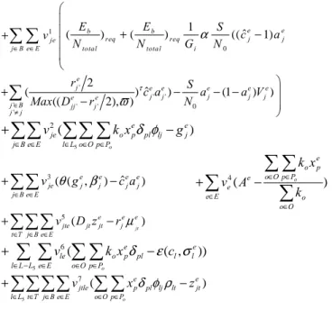
By using the Lagrangean relaxation method, we can transform the primal problem (IP) into the following Lagrangean relaxation problem (LR) where Constraints (1)-(5), (10), and (11) are relaxed. For a vector of non-negative Lagrangean multipliers, a Lagrangean relaxation problem of IP is given by Optimization problem (LR):
(
1 2 3 4 5 6 7)
= , , , , , , je je e jte le jtle jei D v v v v v v v Z ) ( ) ( min i W L l l L l B j j B jh + ∆ c +∆ w ∆∑
∑
∈ ∈1 0 1 ˆ ( b )req ( b )req (( ej 1) ej je j B e E total total i E E S c a v N N G α N ∈ ∈ + − +
∑ ∑
' ' ' ' ' ' 0 ' 2 ˆ ( ) ) (1 ) ) (( 2), ) e j e e e e e j j j j j e e j B jj j j j r c a S a a V Max D r N τ ϖ ∈ ≠ + − − − − ∑
∑∑ ∑∑ ∑
∈ ∈ ∈ ∈ ∈ − + B j eE e j L l o Op P pl lj e p o je k x g v o ) ( 5 2 δ φ∑∑
∈ ∈ − + B j e j E e e j e j e j je g c a v3(θ( ,β ) ˆ )∑
∑
∑ ∑
∈ ∈ ∈ ∈ − + E e O o o O o p P e p o e e k x k A v4( o )∑∑∑
∈ ∈ ∈ − + T t j BeE e e j e jt jt jte D z r jt v5 ( µ )∑ ∑ ∑ ∑
− ∈ ∈ ∈ ∈ − + 5 )) , ( ( 6 L L l eE e l l O o p P pl e p o le kx c v o σ ε δ∑∑∑∑
∑ ∑
∈ ∈ ∈ ∈ ∈ ∈ − + 5 ) ( 7 L l tTj BeE e jt lt lj O o p P pl e p jtle x z v o ρ φ δ subject to: (6)-(9), (12)-(21). where 1 je v , 2 je v , 3 je v , 4 e v , 5 jte v , 6 le v , 7 jtlev are Lagrange multipliers. To solve (LR), we can decompose (LR) into the following five independent and easily solvable optimization subproblems
Subproblem 1: (related to e j cˆ , hj, e j a , e j r and w ) i 0 1 (( ) ) min Bj j ej b req j B e E total i E S h a N GαN ∈ ∈ = ∆ +
∑
∑
1 1 1 ' ' ' ' 2 ? ( ( ) ) ( 2 , ) e j e e j je je j e e e j j B j j j j j r c v v v c Max D r τ ϖ ∈ ≠ − + −∑
1 1 3 0 ˆ e e je je j je j S v v V v c N − + − 1 5 (( ) ) jt e e e b req j je j jte t T total E V v r v N ∈ µ + − −∑
+∆W(wi) (SUB 1)subject to: (6), (9), (12), (13), (17), and
UB c LB e
j≤
≤ˆ ∀ ∈j B e E, ∈ (22)
Base on past experience, we intend to find the lower bound and upper bound of cˆej to improve the efficiency of the subproblem solution, and the gap between the dual
TABLE I. DESCRIPTION OF NOTATIONS
Notation Description Notation Description
Gi The processing gain in the bandwidth state i W The set of total bandwidth
KR Data bit rate Eb The energy BS received
N0 The background noise Ntotal Total noise
α Voice activity R Upper bound of radius of base station j
j
Y The set of radius of base station j
ϖ
A small number(
e)
j e j g β θ ,Minimum number of channels for traffic demand e j
g such that the call blocking probability shall not exceed e
j
β ( , )
e l l
c
ε σ Maximum traffic that can be supported by cl trunks such that
the call blocking probability shall not exceed σle
e j
β Call blocking probability of base station j at state e
jt
µ Indicator function which is 1 if mobile terminal t can be served by base station j and 0 otherwise S
The power that a base station received from the mobile terminal that is homing to it with perfect power control
B The set of candidate location for a base station T The set of mobile terminals E The set of network states (In this report, we only consider the failing possibility of some base stations. One of the
states is that all network components are working.)
e l
σ Call blocking probability of link l required by users
O The set of OD pairs Ae Acceptable coverage ratio on network state e
lt
ρ Indicator function which is 1 if mobile terminal t is one end
of link l δpl
Indicator function which is 1 if link l belongs to path p and 0 otherwise
( )l L l c
∆ Cost function of link l with capacitycl ∆Bj
( )
n Cost function of base station j with capacity n )(w
W
∆ Spectrum w licensing cost φlj Indicator function which is 1 if base station j is one end of link l
M Upper bound on number of users that can be handled by a
base station Po
The set of paths which can support the requirement of OD pair o
e j
V An arbitrarily large number. τ Attenuation factor
j
h Decision variable which is 1 if base station j is decided to build and 0 otherwise
e j
r Decision variable of transmission radius of base station j at network state e
e j
a Decision variable which is 1 if base station j is decided to be activated at network state e and 0 otherwise
e j
cˆ Decision variable of number of users who can be active at the same time in the base station j at network state e
e jt
z Decision variable which is 1 if mobile terminal t is serviced
by base station j and 0 otherwise at network state e δot
Indicator function which is 1 if mobile terminal t belongs to OD pair o and 0 otherwise
Ij The intracell interference Ijj’ The interference from base station j’ to j
o
k User demand of O-D pair o (in Erlangs) Djj’ Distance between base station j and j’
Djt Distance between base station j and mobile terminal t xep Routing decision variable which is 1 if path
p is selected at network state e.
e j
g Decision variable of aggregate flow in base station j on
network state e (in Erlangs) c l Decision variable of capacity assigned for link l.
1
L The set of links which is between two MTSO wi The total bandwidth in the bandwidth state i 2
L The set of links which is between an MTSO and other
systems L3 The set of links which is between an MTSO and other ISPs
4
L The set of links which is between a base station and an
MTSO L5
The set of links which is between a mobile terminal and a base station
solution and primal feasible solution. So, we get Constraint (22). We can assume that only one base station is active and its power radius is maximized. Under this situation, the number of mobile terminals that are covered by the active base station is just the UB if it is smaller than M, the capacity limitation of the equipment. Also, we can assume that all of the base stations are active but one. Under this situation, the number of mobile terminals that are not covered by active base stations and can be covered by the inactive base station is just the LB. First, we can decompose this into |B| independent subproblems. In each subproblem we can decompose this into |E| subproblems again. We can solve these subproblems with the decision tree process.
Subproblem 2: (related to decision variable
z
ejt)∑∑∑
∑∑∑∑
∈ ∈ ∈ ∈ ∈ ∈ ∈ − T t jBeE l L tT j BeE e jt jtle e jt jt jteD z v z v 5 7 5 min (SUB 2)subject to: (8), (15), and
1 e jst j B s S z ∈ ∈ =
∑∑
, if A[e] = 1 E e T t∈ ∈ ∀ , (23)Like SUB 1, we add a redundant constraint (23) to improve the dual solution’s quality. It means that we must find a base station to serve each mobile terminal under the condition that the coverage ratio equals 1. To rewrite (SUB 2), we can get 5 5 e 7 e jte jt jt jtle jt t T j B e E l L t T j B e E v D z v z ∈ ∈ ∈ −∈ ∈ ∈ ∈
∑∑∑
∑∑∑∑
= 5 5 7 ( ) e jt jte jt jtle t T j B e E l L z v D v ∈ ∈ ∈ ∈ −∑∑∑
∑
.Subproblem 3: (related to decision variable
x
p)5 2 min o e je o p pl lj j B e E l L o O p P v k xδ φ ∈ ∈ ∈ ∈ ∈
∑∑ ∑ ∑ ∑
4 ( o ) e o p o O p P e e e E o o O k x v A k ∈ ∈ ∈ ∈ +∑
−∑ ∑
∑
5 6 o e le o p pl l L L e E o O p P v k xδ ∈ − ∈ ∈ ∈ +∑ ∑ ∑ ∑
5 7 o e jtle p pl lj lt l L t T j B e E o O p P v xδ φ ρ ∈ ∈ ∈ ∈ ∈ ∈ +∑∑∑∑ ∑ ∑ (SUB 3)subject to: (7)(14) and
∑
=1∈Po
p e p
x , if A[e] = 1 ∀o∈O,e∈E. (24).
Like SUB 2, we add a redundant constraint (24) to improve the dual solution’s quality. It means that we must find a route for route each OD-pair under the condition that the coverage ratio equals 1.To rewrite SUB 3, we can get
5 2 7 ( ) o e je o pl lj jtle pl lj lt p l L j B t T e E o O p P v k v x δ φ δ φ ρ ∈ ∈ ∈ ∈ ∈ ∈ +
∑∑
∑
∑∑ ∑
5 4 6 4 e o e le o pl e l L L o e E o O v k v k v A k δ ∈ − ∈ ∈ + − + ∑
∑
∑
Subproblem 4: (related to decision variable
c
l)∑ ∑
∑
− ∈ ∈ − ∈ − ∆ 5 5 ) , ( ) ( min 6 L L l e E e l l le L L l l L l c vε c σ (SUB 4) subject to: (18)-(21).Because the value of cl is limited and discrete, we can decompose this into |L| subproblems. To get the optimum solution, we must exhaustively search for all possible cl.
Subproblem 5: (related to decision variable g ) j
∑∑
∑∑
∈ ∈ ∈ ∈ + − B j eE e j e j je B j eE e j jeg v g v ( , ) min 2 3θ β (SUB 5) subject to: g e M j e j, )≤ ( β θ ∀j∈B,e∈E.(25)Constraints (3) and (9) imply Constraint (25). Because the value of ( , e)
j e j
g β
θ is an integer and is limited, we can decompose this into |E|×|B| subproblems. To get an optimal solution, we must exhaustively search for all possible
) , (gej βej
θ .
B. Duality of Planning and Capacity Management Problem
According to the weak Lagrangean duality theorem [2], for any
v
1je,v
2je,v
3je,v
e4,v
5jte,v
le6,v
7jtle≥
0
,Z
D(v
1je,2 je
v
,v
3je,v
e4,v
5jte,v
le6,v
7jtle) is a lower bound onZ
IP. The following dual problem (D) is then constructed to calculate the tightest lower bound.(
1 , 2, 3 , 4, 5 , 6, 7)
max D je je je e jte le jtle
D Z v v v v v v v
Z = (D)
subject to: v1je ,v2je,v3je ,ve4,v5jte ,vle6,v7jtle≥0.
The most common method for solving the dual problem is the subgradient method [3]. Let g be a subgradient of
(
1 ,2,3 ,4,5 ,6 ,7)
jtle le jte e je je je Dv v v v v v vZ . Then, in iteration k of the subgradient optimization procedure, the multiplier vector
)
(
1 2 3 4 5 6 7 , , , , , ,je je e jte le jtle jev v v v v v v =π is updated by πk+1 = πk+tkgk. The step
size tk is determined by ( )
(
2)
/ k h k IP D k t =δ Z −Z π g . ZIPh is theprimal objective function value for a heuristic solution.
IV. GETTING PRIMAL FEASIBLE SOLUTIONS
By using Lagrangean relaxation and the subgradient method as our tools to solve these problems, we can get not only a theoretical lower bound of primal feasible solution, but also some hints to help us get our primal feasible solution under each solving dual problem iteration [6] [8] [12]. If the decision variables calculated happen to satisfy the relaxed constraints, then a primal feasible solution is found. Otherwise, the modification on such infeasible primal solutions can be made to obtain primal feasible solutions; for instance, drop-and-add heuristics. To simplify the process of getting primal feasible solutions, a divide-and-conquer strategy is proposed. We can divide this network design problem into two parts: (1) the mobile terminals homing subproblem and base station configuration subproblem, including the base station should be built or not, and it should be active in every error state or not power control and capacity assignment; (2) the backbone network topology design subproblem and capacity assignment subproblem. In each subproblem, we provide some heuristics to get a primal feasible solution.
A. Heuristics for the Homing and Base Station Configuration Subproblem
To improve our primal feasible solution, we need to find some heuristics to help us. In this part, we try to solve the homing subproblem and the base station configuration subproblem. Base on past experiments, when considering a network design problem with a single component failure state, we can make some decisions about some decision variables in the initialization stage. Taking this problem, for example, for each mobile terminal we can pre-calculate how many base stations can provide service to it without violating the service radius constraint. If there is any mobile terminal only served by “two” base stations, the two base stations must be built.
We continue the solving process with the value of decision variable zjte of each mobile terminal, which is calculated when getting dual solution. With the values of zjte, we can determine the approximate aggregate traffic of each built base station, and we can use these values of approximate aggregate traffic to process the following LR algorithm.
[Algorithm LR]
Step 0. In each failure state, we arrange the built base
stations in descending order of the approximate aggregate traffic.
Step 1. Starting with the base station that has the highest
value of the approximate aggregate traffic, we turn it on in this failure state with the maximum power radius. In the mean time, we turn off the base stations that may violate QoS constraint.
Step 2. We assign all mobile terminals, which are under the
coverage of current base station with such degree of radius and are not assigned yet, to this base station.
Step 3. Then, we consider the other built base stations that
have not been turned off with step 1 and 2.
Step 4. Rearrange the base stations that have not been built
yet in descending order of the approximate aggregate traffic.
Step 5. We decide to build the base station that has the
highest value of the approximate aggregate traffic and turn it on with the maximum power radius in this failure state. In the mean time, we turn off the base stations that may violate QoS constraint.
Step 6. We assign all mobile terminals, which are under the
coverage of current base station with such degree of radius and are not assigned yet, to this base station.
Step 7. Repeat step 4, 5, and 6 until all mobile terminals
have homed to a base station that is built and active in this failure state. If the program gets into an infinite loop and a few mobile terminals are left (the number of mobile terminals / the left mobile terminal > 2), we home them to the base station that has shortest distance between them.
Step 8. Rehome the mobile terminals that are not homed to a
nearest active base station.
Step 9. For each base station, we find the maximum distance
between this base station and its slave mobile terminals. Then we take this value to fit the degree of radius.
Step 10. For each base station, we calculate the actually
aggregate traffic and assign enough capacity.
Step 11. Check the QoS requirement (constraint 1), if it
violates then we give up this iteration.
B. Heuristics for the Tolopogy Design and Capaqcity Assignment Subproblem
In this part, we intend to consider 6 le e E
v
∈
∑ and its length for each link as its weight. Then we use minimum cost spanning tree algorithm to select enough L1 links to build a tree for routing. Then for each base station j, we choose the L4 link, which has the minimum cost, as its candidate link. Then we can calculate the routing path for all OD-pairs on each scenario. According to the aggregate traffic of each link, we assign proper capacity to it under the call blocking rate constraint. Repeat the above processes, consider all network states, to get several values of each link. We choose the maximum volume of capacity of each link, which is calculated on each network state, as our primal solution.
V. COMPUTATIONAL EXPERIMENTS A. Experiment Environment
Because of the complexity of this network design problem, we cannot get a tighter lower bound by solving the Lagrangean relaxation problem iteration by iteration. Although we cannot get a tighter lower bound, this powerful methodology provides a lot of hints to help us get a primal feasible solution. In order to demonstrate that our heuristics are good enough, we also implement a simple algorithm (denote SA) to compare with our heuristics.
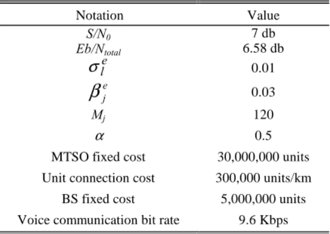
TABLE II. GIVEN PARAMETER FOR EXPERIMENTS
Notation Value S/N0 7 db Eb/Ntotal 6.58 db e l
σ
0.01 e jβ
0.03 Mj 120 α 0.5MTSO fixed cost 30,000,000 units
Unit connection cost 300,000 units/km
BS fixed cost 5,000,000 units
Voice communication bit rate 9.6 Kbps
TABLE III. EXPERIMENTAL SCENARIOS
Error State
Case MTSO BS MT O-D
Pair Traffic demand* 1 3 15 40 20 0.1 2 3 15 40 20 1.5 0/1 3 3 15 40 20 3.0 A 3 15 40 20 1.5 B 3 30 40 20 1.5 0 only C 3 40 40 20 1.5 * in Erlangs
B. Experimental Parameters and Results
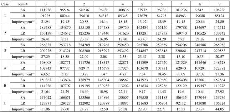
The parameters referring to previous works of Um [4], Lin [6], Wu [8], and Lee [12] are listed in Table II. Table III specifies a number of experimental scenarios. All experiments are coded in Java and performed on a dual Pentium III 1G MHz PC running Microsoft Windows 2000 Advance Server with 2GB DRAM. Results analysis of all experimental scenarios is also enumerated in Table IV, in which Case 1 and 2 take around 1-1.5 hours for 1000 iterations. If we ignore the consideration of error states, i.e. only considering the error state 0, the time complexity is considerably decreased. Case A, B, and C only take around 3, 13, and 20 minutes, respectively, for 1000 iterations in experiments. The statistic of approximated computational time is reported in Table V.
Obviously, in Table V, it is more time-consuming if we take into survivability account in network planning. Be more efficiently, it is suggested that in the stage of network planning and design, the normal condition (without considering failure states) is appropriate. Furthermore, a new model jointly considering survivability and capacity management can be developed when it is needed.
Generally speaking, a basic approach to provisioning survivable services is duplication of base stations. This implies that it requires double expenses for constructing a survivable network. By using proposed approach of modeling survivable network, as we can see the comparison of case 2 and case A in Table VI, it takes around more 36.194% cost to guarantee survivability rather than 100%.
VI. CONCLUSIONS
In this report, we present an approach to designing and managing a DS-CDMA wireless communication network. We can express our achievements in terms of formulation and performance. In terms of formulation, we model a mathematical expression to describe the overall DS-CDMA wireless communication network design and management problem. We consider both regular size cell and non-uniform traffic demand to make this report more generic. An average interference model is discussed. In terms of performance, our Lagrangean relaxation based solution has more significant improvement than other intentional algorithms. Besides, the following subjects may deserve future investigation. First, sectorization is widely used in wireless communication system. Second, to cover both uplink and downlink is another topic worth further investigation. Third, a new frequency planning strategy
should be designed to improve the system performance. Adding a new frequency planning strategy into our model would be an interesting work. Fourth, since many applications will be developed in the future, how to transfer our model to fit the other traffic models would be an important task.
REFERENCES
[1] A.O. Fapojuwo, “Radio Capacity of Direct Sequence
Code Division Multiple Access Mobile Radio Systems”, IEE Proceedings Communications, Speech and Vision, Vol. 140, pp. 402-408, 1993.
[2] Fisher and L. Marshall, “The Lagrangian Relaxation Method for Solving Integer Programming Problems”, Management Science, Vol. 27, pp.1-18, 1981
[3] A.M. Geoffrion, “Lagrangean Relaxation and Its Use in Integer Programming”, Math. Programming Study, Vol. 2, pp. 82-114, 1974.
[4] M. Held, P. Wolfe and H.D. Crowder, “Validation of Subgradient Optimization”, Math. Programing, Vol. 6, pp. 62-88, 1974.
[5] H.Y. Um; S.Y. Lim, “Call Admission Control Schemes for DS-CDMA Cellular System Supporting an Integrated Voice/Data Traffic”, ISCC '98. Proceedings Computers and Communications, pp. 365-369, 1998. [6] F.Y.S. Lin and C.Y. Lin, “Integrated Planning and
Management of Survivable Wireless Communications Networks,” in Proc. APCC/OECC, Vol. 1, pp. 541 -544, 1999.
[7] S.M. Shin, C.H. Cho and D.K. Sung,
“Interference-based Channel Assignment for DS-CDMA Cellular Systems”, IEEE Transactions on Vehicular Technology, Vol. 48, pp. 233-239, 1999.
[8] S.Y. Wu and F.Y. S. Lin, “Design and Management of Wireless Communications Networks,” in Proc. INFORMS CIST, pp. 284-306, Cincinnati, USA, May 1999.
[9] D. Dahlhaus and Z. Cheng,” Smart antenna concepts with interference cancellation for joint demodulation in the WCDMA UTRA uplink”, Spread Spectrum Techniques and Applications, Vol. 1, pp. 244-248, 2000.
[10] M.A. Hernandez, G.J.M. Janssen, and R. Prasad, ”Uplink performance enhancement for WCDMA systems through adaptive antenna and multi-user detection,” in Proc. IEEE 51st VTC-Spring, vol. 1, pp. 571-575, Tokyo, Japan , 2000.
[11] A.P. Snow, U. Varshney and A.D. Malloy, “Reliability and survivability of wireless and mobile networks,” Computer, Vol. 33, Issue: 7, pp. 49 –55, July 2000. [12] S.H. Lee, “DS-CDMA Wireless Communications
Network Design and Management”, M.S. thesis, Department of Information Management, National Taiwan University, Taipei, Taiwan, 2001.
[13] W.C.Y. Lee, “Overview of Cellular CDMA”, IEEE Transactions on Vehicular Technology, Vol. 40, pp. 291-302, 1991.
TABLE IV. EXPERIMENTAL RESULTS Case Run # 0 1 2 3 4 5 6 7 8 9 SA 111236 95594 96236 96236 100836 83932 96236 101236 95421 106236 LR 91225 80244 79610 84312 85345 73679 84795 84963 79080 85124 1 Improvement* 21.94 19.13 20.88 14.14 18.15 13.92 13.49 19.15 20.66 24.80 SA 189788 134870 155150 174788 159750 162484 155150 179788 134697 145512 LR 150139 124642 125236 149440 141620 113281 124833 169740 110525 130742 2 Improvement* 26.41 8.21 23.89 16.96 12.80 43.43 24.29 5.92 21.87 11.30 SA 266325 253718 254289 219768 259450 265706 259859 254206 248586 265958 LR 209225 214321 208280 215297 253492 214857 253818 220861 247714 220583 3 Improvement* 27.29 18.38 22.09 2.08 2.35 23.67 2.38 15.10 0.35 20.57 SA 168008 102771 111756 118317 122871 111809 127650 121529 141646 148528 LR 102743 97737 92917 116599 117324 103678 107771 62940 107291 122382 A Improvement* 63.52 5.15 20.28 1.47 4.73 7.84 18.45 93.09 32.02 21.36 SA 150367 133874 138979 145304 138567 143923 139650 145408 132061 152584 LR 114226 107707 119195 130932 113202 131834 125286 122129 119357 119278 B Improvement* 31.64 24.29 16.60 10.98 22.41 9.17 11.43 19.6 10.64 27.92 SA 137022 166651 153366 134896 150605 149550 131183 106415 177044 153736 LR 123371 129127 122902 120389 118885 121683 106904 92112 143080 106724 C Improvement* 11.06 29.60 24.79 12.50 26.68 22.90 22.71 15.53 23.74 44.05
*Improvement is expressed by (SA-LR)/LR*100%
TABLE V. COMPARISON OF COMPUTATION TIME (SEC)
Case 1 2 3 A B C SUB 1 30 30 30 1 16 16 SUB 2 300 300 300 16 30 47 SUB 3 700 700 700 47 100 140 SUB 4 1 1 1 1 1 1 SUB 5 1 1 1 1 1 1 Subgradient 3300 3370 3200 235 600 890 Solving Primal 16 16 24 1 16 16 Iteration 1000 1000 1000 1000 1000 1000
TABLE VI COST COMPARISON OF CONSIDERING SURVIVABLE FACTOR OR NOT
Run # 0 1 2 3 4 5 6 7 8 9
LR of Case 2 150139 124642 125236 149440 141620 113281 124833 169740 110525 130742 LR of Case A 102743 97737 92917 116599 117324 103678 107771 62940 107291 122382
More cost (%) 46.13 27.53 34.78 28.17 20.71 9.26 15.83 169.69 3.01 6.83