運用關係萃取策略於動態社群探勘之研究

(1)

國

立

交

通

大

學

資訊科學與工程研究所

碩

士

論

文

運用關係萃取策略於動態社群探勘之研究

Dynamic Community Detection via Relationship

Extraction Strategy and Community Pedigree Mapping

研究生：彭誠毅

指導教授：李素瑛教授

(2)

運用關係萃取策略於動態社群探勘之研究

Dynamic Community Detection via Relationship Extraction Strategy and

Community Pedigree Mapping

研究生：彭誠毅 Student：Cheng-Yi Peng

指導教授：李素瑛 Advisor：Suh-Yin Lee

國立交通大學

資訊科學與工程研究所

碩士論文

A Thesis

Submitted to Institute of Computer Science and Engineering College of Computer Science

National Chiao Tung University in partial Fulfillment of the Requirements

for the Degree of Master

in

Computer Science

July 2011

Hsinchu, Taiwan, Republic of China

(3)

i

運用關係萃取策略於動態社群探勘之研究

研究生：彭誠毅指導教授：李素瑛

國立交通大學資訊科學與工程研究所

摘要

近來在動態社會網路上，因為社群演化的廣大應用，動態社群的問題已經引起重大的關注。多數潛在的社會現象實際上可經由分析社群網路結構萃取出來。雖然在動態社群上已有多數的研究發表。它們一般而言均針對一連串的互動圖作社群分群，一連串的互動圖是通常用來表現動態社群網路的一種方式。然而互動圖展露在人與人之間的關係可能是不夠充足，因為它只是在一個時間切片上的快照。在這時間切片上兩人若沒有互動發生，並不代表這兩人沒有關係。本篇論文提出一個新穎的演算法，EPC(關係萃取和社群氏族的社群探勘者)，可被用來探勘社群演化。我們提出了一個關係萃取策略，在一個時間窗內產生出關係圖。EPC 架構於關係圖來產生社群分群，且利用社群氏族對映來發掘出動態社群在動態社群網路上的演化。實驗結果在合成資料和真實數據中顯示 EPC 的結果不僅在準確度比之前的方法佳，且在彈性和平滑程度也勝過之前的方法。檢索詞：動態社群，關係萃取，衰減權重函數，社群氏族。

(4)

ii

Dynamic Community Detection via Relationship Extraction

Strategy and Community Pedigree Mapping

Cheng Yi Peng Suh-Yin Lee

Institute of Computer Science and Information Engineering

National Chiao-Tung University

Abstract

Recently, considerable attention has been paid to the issue of dynamic community in dynamic social network due to its widespread applications. Many potential social phenomena, in practice, can be extracted by analyzing the dynamic social structure over time. Although there have been many recent studies proposed on dynamic community, these works, generally, partition the community based on a sequence of interaction graphs, which is usually applied to express a dynamic social network. Nevertheless, the interaction graph may be insufficient to reveal the relationship among individuals, since, in a snapshot of time slice, no interaction among individuals does not indicate no actual relationship. In this thesis, a novel algorithm EPC, which stands for relationship Extraction and community Pedigree mapping Community miner, is developed to mine the evolution of community. We present a Relationship Extraction strategy to construct a relationship graph within a defined observation window. EPC partitions communities based on relationship graph and uses proposed Community Pedigree Mapping method to discover the evolution of dynamic community in dynamic social network. The experimental results on synthetic and real datasets

show that EPC not only

significantly outperforms the prior studies in accuracy but also possesses

graceful scalability and smoothness.

(5)

iii

Index terms: dynamic community, relationship extraction, decay weight

(6)

iv

ACKNOWLEDGEMENT

I greatly appreciate the kind guidance of my advisor, Prof. Suh-Yin Lee. She not only helps with my research but also takes care of me. Her graceful suggestion and encouragement help me forward to complete this thesis.

Besides, I want to give my thanks to all members in the Information System Laboratory for their suggestion and instruction, especially Mr. Yi-Cheng Chen, Ms. Chao-Ying Wu, Mr. Wang-Zen Wang, Mr. Fan-Chung Lin and Mr. Li Yen Qua.

Especially I would express my thanks to Ms. Yu-Ru Lin for providing FacetNet code, Ms. Heli Sun for providing SHRINK code and Mr. Alan Mislove for providing the Facebook dataset.

Besides, I would express my thanks to the nicest and most beautiful lady Ms. Hui- yu Liou who accompanies me and always give me a happy smile.

Finally I would like to express my deepest appreciation to my parents. This thesis is dedicated to them.

(7)

v

List of Figures

Figure 2-1 Interaction data example...7

Figure 2-2 Community partition produced by CPM...8

Figure 2-3 Evolution Net...9

Figure 2-4 Concept of temporal smoothness...10

Figure 2-5 Mixture model(a) the original graph Gt (b) the bipartite graph with two communities c1 and c2 (c) How to approximate an edge (G42).[3]...12

Figure 2-6 Flowchart of PD-Greedy...13

Figure 2-7 Community partition of temporal smoothness...14

Figure 4-1 Flowchart of EPC, “relationship Extraction and community Pedigree dynamic Community miner” ...18

Figure 4-2 Framework of EPC, “relationship Extraction and community Pedigree dynamic Community miner”...19

Figure 4-3 Example of determining the relationship strength...21

Figure 4-4 Using the EQL weight function to construct the Relationship graph RG2 of sample interaction data of Fig 2-1...22

Figure 4-5 Normalized Decay Weight Function (wr=2)...23

Figure 4-6 Relationship strength curve between u and v by extraction from the interaction data of Fig 4-2 based on Normalized Equal Weight Function (wr=2)...24

Figure 4-7 The Relationship strength curve of the interaction data of Fig4-2 based on Normalized Linear Decay Weight function (wr=2)...25

Figure 5-1 (a) Sample network G (b) Connected cluster of Sample network G...28

Figure 5-2 All Dense Pairs within the sample network G in Fig 5-1(a)...29

Figure 5-3 Round 1(a): Find all Dense pairs in G (b)Δ Q>0, Shrink...32

Figure 5-4 Round 2(a): Find all Dense pairs in G (b)Δ Q>0, Shrink...32

(11)

ix

Figure 5-6 Algorithm of SHRINK...33

Figure 5-7 Algorithm of SCAN...34

Figure 5-8 Algorithm of GSCAN...35

Figure 6-1 Calculation example of community similarity ...37

Figure 6-2 (a) Merge example (b) Split example...37

Figure 6-3 Example of evolution of communities...39

Figure 6-4 (a) Evolution net (b) Pedigree of single Community ...40

Figure 6-5 Algorithm of EPC...42

Figure 7-1 Parameter of FacetNet: α ...47

Figure 7-2 Parameters of PD-Greedy: α , μ on dataset SYN-FIX-VOD_3...48

Figure 7-3 Parameters of PD-Greedy: α , μ on dataset SYN-FIX-VOD_5...48

Figure 7-4 Parameters of PD-Greedy: α , μ on dataset SYN-VAR-COD_0_3_REG..49

Figure 7-5 Parameters of PD-Greedy: α , μ on dataset SYN-VAR-COD_0_5_REG..49

Figure 7-6 The EXP weight function under different observation eyeshot wr...50

Figure 7-7 Parameters of EPC-SHRINK: observation eyeshot, decay weight functions on dataset SYN-FIX-VOD_3...51

Figure 7-8 Parameters of EPC-SHRINK: observation eyeshot, decay weight functions on dataset SYN-FIX-VOD_5...51

Figure 7-9 Parameters of EPC-GSCAN: observation eyeshot, μ on dataset SYN-VAR-COE_0_3_RAN...52

Figure 7-10 Parameters of EPC-GSCAN: observation eyeshot, μ on dataset SYN-VAR-COE_0_5_RAN...53

Figure 7-11 Parameters of EPC-GSCAN: decay weight functions on dataset SYN-VAR-COE_0_3_RAN...53 Figure 7-12 Parameters of EPC-GSCAN: decay weight functions on dataset

(12)

x

SYN-VAR-COE_0_5_RAN...54

Figure 7-13 Accuracy comparison on dataset SYN-FIX-VOD_3...55

Figure 7-14 Accuracy comparison on dataset SYN-FIX-VOD_3...55

Figure 7-15 (a) Accuracy comparison on dataset SYN-VAR-COE_0_3_REG...56

(b) Accuracy comparison on dataset SYN-VAR-COE_0_5_REG...56

(c) Accuracy comparison on dataset SYN-VAR-COE_0_3_RAN...56

(d) Accuracy comparison on dataset SYN-VAR-COE_0_5_RAN...57

Figure 7-16 Smoothness comparison on dataset SYN-FIX-VOD_3...58

Figure 7-17 Smoothness comparison on dataset SYN-FIX-VOD_5...58

Figure 7-18 (a) Smoothness comparison on dataset SYN-FIX-COE_0_3_REG...59

(b) Smoothness comparison on dataset SYN-FIX-COE_0_5_REG...59

(c) Smoothness comparison on dataset SYN-FIX-COE_0_3_RAN...59

(d) Smoothness comparison on dataset SYN-FIX-COE_0_5_RAN...60

Figure 7-19 Execution time of EPC-SHRINK, EPC-GSCAN and PD-Greedy w.r.t different input size...60

Figure 7-20 Memory usages of EPC-SHRINK, EPC-GSCAN and PD-Greedy...61

Figure 7-21 Result of Enron email dataset using EPC-SHRINK...62

Figure 7-22 Smoothness quality result on Enron email dataset...62

Figure 7-23 Result of Facebook dataset using EPC-SHRINK...63

Figure 7-24 Smoothness quality result on Facebook email dataset...64

Figure 7-25 Result of DBLP dataset using EPC-SHRINK...64

(13)

xi

List of Tables

Table 7-1 Parameters of SYN-FIX...43 Table 7-2 Parameters of SYN-VAR...44 Table 7-3 Synthetic datasets generated by SYN-FIX and SYN-VAR...45

(14)

1

Chapter 1. Introduction

In recent years, social network analysis in e-commerce, social science and computer science has received significant attention. A social network is a social structure made up of individuals, which are tied by one or more specific types of relationship or interdependency, such as friendship, co-authorship, common interest or financial exchange. Clustering similar individuals into a group has been a big challenge. A cluster in a social network is typically called a community. Traditional static methods discovered communities using the aggregate interaction data and ignored the effect of time. However, social networks are dynamic and evolve over time. With the increasing popularity of social network websites, the use of dynamic social network analysis has increasingly been the focus of study in recent years.

Two major issues of dynamic community need to be addressed:

(1) Community discovery: Which nodes should be associated with each other to

become a community at each timestamp? (2) Evolution of community: How to explain the evolution of community partition from previous timestamp to current timestamp?

Traditional methods of discovering dynamic communities such as [6, 7] are called two-stage approach. The community partition is detected at each timestamp using the

interaction graph and the evolutions of communities between two consecutive timestamps are inferred successfully. However, the community partition discovered by current interaction data could distort the real community structure. The community partition presumed that there is no relationship between individual pairs while no interactions occur between them.

Recently, a new concept of temporal smoothness was proposed [1] based on two points of view. (1) Each community partition in the time sequence should be similar to the community partition at the previous timestamp. (2) The community partition should accurately reflect the change of the interaction networks. The concept of temporal smoothness tries to discover the communities which not only consider about interaction data

(15)

2

of current timestamp but also historical interaction data to improve the weakness of two stage approach.

However, the methods [1, 2, 3, 5] based on temporal smoothness have the following drawbacks. It is a big issue that the community partition should well reflect the previous interaction data more or a little more reflect the current interaction data. If the community partition always well reflects the previous interaction data more, the new change of social network would be hard to detect. On the other hand, the community partition would be more similar to the community partition based on two-stage approach and have the same weakness as two-stage approach. This setting of temporal smoothness has a great effect on the result of the methods based on temporal smoothness.

Concerting the evolution of community, current methods [6, 13, 3, 5] focused on that one community of previous timestamp maps to one community of current timestamp (one-to-one mapping). We argue that mapping is not suitable for real dynamic community because mapping of communities is not always one-to-one.

In this thesis, we propose EPC, “relationship Extraction and community Pedigree dynamic Community miner”, which produces the community partition taking into account the evolution of community. Instead of interaction data, we proposed the Relationship Extraction strategy which constructs a weighted graph for each timestamp and the weight indicates the relationship strength between individuals; we use two current static clustering algorithms, SHRINK [12] and GSCAN [5], to discover the community based on Relationship graph. We also proposed the Community Pedigree mapping which uses a realistic way to explain the evolution of dynamic community.

The Relationship Extraction strategy produces the relationship graph which not only references the historical interaction data but also the ongoing interaction data. The relationship graph not only represents much realistic relationship between individuals but also express the dynamic property in relationship graph. The Relationship Extraction strategy

(16)

3

combines the normalized decay weight function to simulate the change of relationship strength between individuals. The Community Pedigree mapping extends the human pedigree to illustrate the evolution of community over time. The states of a community could be Birth, Death, Alive, Child and Fission. Using the community pedigree mapping, we could simply determine the evolution of community.

In synthetic data experiment, our algorithm EPC not only has higher accuracy but also more smoothing than previous algorithms. The EPC also expresses the property of linearly scalability. We also apply EPC on real datasets, Enron email dataset; Facebook dataset and DBLP dataset. All datasets show the change of community partition in real dynamic social network is quite low. The change rates of communities in co-authorship and friendship are higher than the change rate in company since the variation of company network is lower than friendship network and co-authorship network.

In summary, the contributions of this thesis are as follows:

(1) We propose a new technique of data smoothing, Relationship extraction strategy, to produce a relationship graph. We discover community partition using the relationship graph instead of current interaction to overcome the weakness of two-stage approach. The relationship graph not only represents much realistic relationship between individuals but also express the dynamic property in dynamic social network.

(2) We propose a new matching technique, Community Pedigree mapping, which extends the point of human pedigree to explain evolution of community.

(3) We propose EPC, “relationship Extraction and community Pedigree dynamic Community miner”, which has not only higher accuracy but also better smoothing than

previous methods no matter the noise level of data is high or low.

(4) EPC is linearly scalable both on the execution time and memory usage.

The rest of this thesis is organized as follows. Chapter 2 provides the related work and motivation. Chapter 3 presents the notation and problem definitions. Chapter 4 introduces the

(17)

4

Relationship graph strategy. Chapter 5 describes the SHRINK [12] and GSCAN[5] cluster algorithms. Chapter 6 presents the evolution of community and the proposed algorithm EPC. Chapter 7 presents the experiments and performance study. The conclusion and future work is in chapter 8.

(18)

5

Chapter2

Related Works and Motivation

In this section, we introduce the related works and motivation of this thesis. We first introduce the community detection technique in static graphs and then describe that in dynamic graphs where the dynamic graphs could change over time. Section 2-3 describes the motivation of this thesis.

2.1 Community Detection in Static Graphs

In the study of community detection in a single static graph which doesn’t change over time, several approaches have been proposed on static graph.

Graph Partitioning approach consists of dividing the vertices into k groups of predefined size, such that the number of inter-edges between the groups is small [29]. The Kernighan -Lin algorithm is one of the earliest methods. Another popular technique proposed by Barnes et al is the spectral bisection method, which is based on the properties of the spectrum of the Laplacian matrix. The Laplacian matrix L= D-A where D is the diagonal matrix whose element Dii equals the degree of vertex i and A is the adjacency matrix of the graph. In

particular, the eigenvector corresponding to the second smallest eigenvalue is used for graph bipartitioning.

However, the Graph partitioning based methods need to predefine the number of clusters or the size of clusters at the beginning and the predefined parameter has great effect upon the result of graph partitioning.

In modularity-based approach, the modularity measure has been widely used in community discovery for evaluating the quality of network partitions. Modularity-based approach [18, 19] assumes high value of modularity indicates good partitioning and the partition corresponding to its maximum modularity score on a given graph should be the best.

However, detection of a community whose size is smaller than a certain size is impossible. This serious problem is famously known as the resolution limit of

(19)

6 modularity-based algorithms [10].

The density based approach applies a local cluster criterion. Clusters are regarded as regions in the data space in which the objects are dense, and which are separated by regions of low object density. Density of intra-edges is used to partition graph into clusters. Xu et al [21] proposed the Structural Clustering Algorithm for Network (SCAN). SCAN [21] needs two predefined parameters minimum similarity threshold ( ) and minimum neighbors of core node ( ) which limits that a core node has at least neighbors whose similarities are more than minimum similarity threshold ( ). Each cluster should contain at least one core node inside.

SCAN is an efficient structural network clustering algorithm while the predefined parameters are appropriate.

However, SCAN [21] requires the predefinition of the minimum similarity parameter ( ) and minimum core size ( ) and the setting of parameters would huge affect the result of

cluster partitions.

Recently a structural clustering algorithm called SHRINK was proposed by Huang et al [12] to overcome the problem of predefining parameters ( and ) of density-based clustering algorithm. Through the experiment, SHRINK was proven to be an efficient, parameter free and higher accuracy algorithm while comparing with the modularity-based approach [18, 19].

2.2 Community Detection in Dynamic Graphs

Real social networks change over time so the community partition changes over time. So community detection in dynamic graphs would be more realistic than community detection in static graphs. Several approaches for discovering dynamic communities have been studied in dynamic social networks. We would illustrate the concept of these approaches.

2.2.1 Two-Stage Approach

Two-stage approach has two steps: (1) Community partition is detected at each

(20)

7

different timestamps. (2) While the relationships between the communities of two consecutive timestamps are determined, the community mapping of two consecutive timestamps are inferred successfully.

Palla et al [6] proposed a method called Clique Percolation Method (CPM) to analyze the real dynamic network such as co-authorship network and mobile phone network. The CPM tries to find all k-cliques that can be reached from each other through a series of adjacent k-cliques where the adjacency means sharing k-1 nodes. The adjacency k-cliques are considered as community in [6]. The community mapping of two consecutive timestamps are dependent on their relative node overlapping. They first described the events in community evolution including Birth, Death, Merging, Splitting, Growth and Contraction. They have shown that the lifetime of communities in these networks depends on the dynamic behavior of these communities, with large groups that alter their behavior persisting longer than others. On the other hand, small groups were found to persist longer if their membership remained unchanged [6].

Sun et al [7] considered dynamic networks such as Network traffic, email and cell-phone as bipartite graphs which treat source and destination separately. GraphScope [7] is based on the principle of Minimum Description employs (MDL) and employs lossless encoding scheme for a graph stream. The encoding scheme takes into account both the community structure and the community change in order to achieve a concise description of the data.

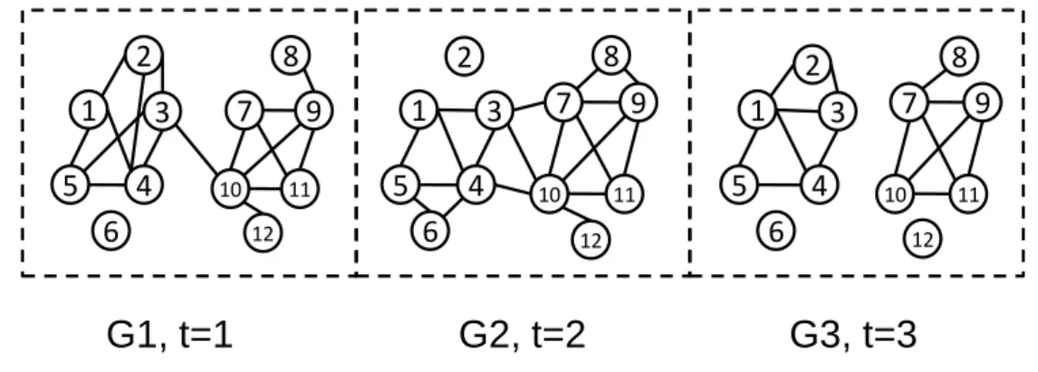
Figure 2-1 Interaction data example

G1, t=1 G2, t=2 G3, t=3

7 5 1 4 3 2 6 8 9 10 11 12 7 5 1 4 3 2 6 8 9 10 11 12 7 5 1 4 3 2 6 8 9 10 11 12

(21)

8

We use Fig 2-1 and Fig 2-2 to illustrate the weakness of methods based on the two stage approach. Given the interaction data as shown in Fig 2-1, a node indicates an individual and

an edge ( u, v ) indicates the interaction occurs between u and v. The community partition result of CPM [6] is shown in Fig-2-2. There are two communities discovered in time 1, one community discovered in time 2 and two community discovered in time 3.

Figure 2-2 Community partition produced by CPM

While the interaction data change frequently, the community partition also change frequently. The node 2 is covered by a community at time 1 and time 3. However, the individual 2 disappeared at time t=2 because individual 2 has no interaction with other individuals at time t=2. There should be some relationship strength between individual 2 and other individuals even though no interactions occur at time t=2.

However, the methods [6,7] based on the two-stage approach presume that there is no relationship between individual pairs while no interactions occur between them and it often results in community structure with significant changes [3].

While the community partitions at all timestamps have been produced, how to illustrate the evolution of community is another issue. In the studies of evolution of community, Palla et al [6] proposed a point of view that the basic operation in a community life should contains birth, death, growth, contraction, merge and split.

Asur et al. [13] considered the issue of community evolution and they defined their own community similarity function. They proposed five critical events such as Continue, K-merge, K-split, Form and Dissolve to illustrate the evolution of communities between two

G₁, t=1 G₂, t=2 G₃, t=3 7 5 1 4 3 2 6 8 9 10 11 12 7 5 1 4 3 2 6 8 9 10 11 12 7 5 1 4 3 2 6 8 9 10 11 12

(22)

9 consecutive timestamps.

Lin et al [3] proposed the Evolution net which is a bipartite graph to illustrate all relationship between the communities of every two consequent timestamps. However, Lin et al [3] didn’t illustrate how a community evolution over time. Kim et al [5] also propose a heuristic mapping algorithm based on mutual information.

However the above methods [6, 13, 3, 5] made effort in the mapping a community at previous timestamp to a community at current timestamp ( 1-1 mapping problem ). We use Fig 2-3 to illustrate the point of view.

Figure 2-3 Evolution Net

The evolution net shown in Fig 2-3 is a bipartite graph from t-1 to t. There are 5 communities (A, B, C, D, E) at t-1 and 5 communities (F, G, H, I, J) at t. A node indicates a community and an edge from a community of t-1 to community of t indicates that there is a relationship between these two communities where the edge weight indicates the similarity between them. The community B having relationships with communities F and G could be considered as community B being divided into two parts, one part of B merges with community A into community F at timestamp t; the other part of B and one part of C are merged into community G. The merge and split operations of communities could happen at the same time.

Although the similarities between communities are determined and are shown an edge weight in Fig 2-3, there is no indication community F is a split part of B or F is a growth of community A. Similarly, we do not know if community C is dead while community G matches with community B. It is judged that the one to one mapping is not suitable for real

t F

A

B

C

1 0.7 0.3

t-1

G

0.7

H

0.3

D

E

I

J

1

(23)

10 dynamic networks.

2.2.2 The approach of Evolutionary Clustering

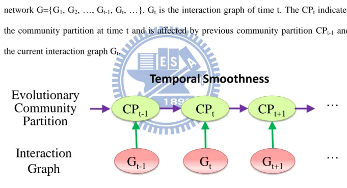
The approach of Evolutionary clustering was first proposed in [1] taking into account the concept of temporal smoothness. Each community partition in the time sequence should be similar to the community partition at the previous time slice. The community partition should accurately reflect the change of the interaction graph. For evolution clustering, [1] adopted the two widely used clustering algorithms, k-means and agglomerative hierarchical clustering incorporating temporal smoothness.

Fig 2-4 shows the details of the concept of temporal smoothness. Given the dynamic network G={G1, G2, …, Gt-1, Gt, …}. Gt is the interaction graph of time t. The CPt indicates

the community partition at time t and is affected by previous community partition CPt-1 and

the current interaction graph Gt.

Figure 2-4 Concept of temporal smoothness

In order to measure the quality of community partition based on the concept of temporal smoothness, the objective function is defined:

(1)

Consider all possible community partitions AP = { , , …, ,…}. For each community partition , the snapshot cost SC() measures the similarity between the interaction graph Gt and . The temporal cost TC() measures the similarity between the

previous community partition CPt-1 and . While the SC() is lower, the quality of snapshot

Temporal Smoothness

G

_t-1

G

_t

G

_t+1

CP

_t-1

CP

_t

CP

_t+1

…

Interaction

Graph

Evolutionary

Community

Partition

(24)

11

is higher. While the TC() is lower, the quality of temporal smoothness is higher. The optimal community partition CPt= | . The parameter α controls the

emphasis of the result of community partition. While α =1, the community partition CPt

would be the same as community partition discovered in Gt . On the other hand, the CPt

would be the same as CPt-1 whileα =0.

Chi et al [2] extended the concept of temporal smoothness and considered that the characteristic change of dynamic community contains both long-term trend drift and short-term variation due to noise. They proposed two evolutionary spectral clustering algorithms called Preserving Clustering Quality (PCQ) and Preserving Clustering Membership (PCM). Their experiment shows that PCQ and PCM are less sensitive to short-term noises while at the same time are adaptive to long-term cluster drifts. The spectral clustering uses the eigenvectors of Laplacian matrix for clustering the graph nodes. The

Laplacian matrix L= D-A where D is the diagonal matrix whose element Dii equals the degree

of vertex i and A is the adjacency matrix of the graph.

Lin et al [3], who are the first critic, argue that the methods of two-stage approach are inappropriate in applications with noise data. They considered an individual could be assigned to more than one community so they further assumed that each interaction graph Gt is

combined effect by community partition CPt. They extended a mixture model [30] and

incorporated the concept of temporal smoothness. The mixture model is a probabilistic model for representing the presence of sub-populations within an overall population, without requiring that an observed data-set should identify the sub-population to which an individual observation belongs.

Given Gt as the interaction graph at time t and assume there are k communities at time t.

Mixture model assumes that the edge Gij of Gt is combined effect due to all the k communities

(25)

12

to the r-th community, and are the probabilities that an interaction in r-th

community involves node i and node j, respectively. Written in a matrix form, we have where is a n × k non-negative matrix and indicates the probability of node i belonging to community j. In addition, is a k × k non-negative diagonal matrix with where indicates . We use Fig 2-5 to illustrate the mixture model [3].

(a) (b) (c)

Figure 2-5 Mixture model(a) the original graph Gt (b) the bipartite graph with two communities c1 and c2 (c) How to approximate an edge (G42).[3]

In Fig. 2-5, there are 6 nodes and 2 communities. For a general graph Gt in Fig 2-5(a), we use a special bipartite graph Fig 2-5(b) to approximate Gt. Note that (b) has two more nodes, i.e., c1 and c2, corresponding to the two communities. In (c), we show how an edge G34 is generated in the mixture model as the sum of and [3].

The Kullback-Liebler divergence was used to measure the difference between two community partitions P and Q to reconstruct the defined cost function. They proposed “A Framework for Analyzing Communities and EvoluTions in dynamic NETworks” (FacetNet), defined the Community net and Evolution net to represent the community structure and evolutions.

However, the methods in [ 1, 2, 3 ] assign a fixed number of communities over time and do not allow arbitrary start/stop of community over time [5].

Kim et al [5] overcome the problems of fixed number of community and arbitrary

v2

v1

v5

v4

v3

c1

c2

v6

v2

v1

v5

v4

v3

v6

v2

v1

v5

v4

v3

c1

c2

v6

Λ

₁

Λ

₂ X₃₁ X₄₁ X₄₂ X₃₂

G

₄₂

(26)

13

start/stop of community. They first model a dynamic network as a collection of particles called nano-community, and a community as a densely connected subset of particles, called a quasi l-clique-clique. They proposed a greedy algorithm called “a Particle-and-Density Based Evolutionary Clustering Method” (PD-Greedy). PD-Greedy extends density based clustering [20, 21] and incorporates with the concept of temporal smoothness. They used a cost embedding technique to efficiently find temporally smoothed local clusters of high quality.

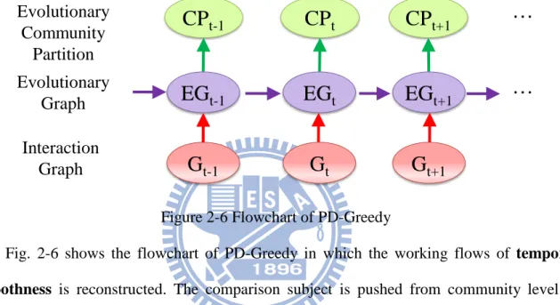
Figure 2-6 Flowchart of PD-Greedy

Fig. 2-6 shows the flowchart of PD-Greedy in which the working flows of temporal smoothness is reconstructed. The comparison subject is pushed from community level to

down data level. At each timestamp, an evolution graph (EGt), which reference both previous

evolution graph (EGt-1) and current interaction graph (Gt), is produced. Then the community

partition based on the EGt is discovered.

However, the methods including PD-Greedy [1, 2, 3, 5] based on temporal smoothness have several drawbacks. The parameter α of cost function might affect the community partition produced by the methods based on temporal smoothness.

Assume the interaction data is the same as in Fig 2-1, the previous community partition CP1 is shown on the left of Fig 2-7 and the snapshot partition of G2 is shown on the right of

Fig 2-7.

G

_t-1

G

_t

G

_t+1

CP

_t-1

CP

_t

CP

_t+1

…

Interaction Graph Evolutionary Graph

EG

t-1

EG

t

EG

t+1 Evolutionary Community Partition

…

(27)

14

Figure 2-7 Community partition of temporal smoothness

Based on temporal smoothness, the community partition CP2 is not only similar to CP1

but the snapshot partition of G2. if the parameter α of the cost function of the concept of

temporal smoothness is close to one, the CP2 is similar to the result of two-stage-approach and

has the same weakness of two-stage approach. On the other hand, if the parameter α of the cost function of the concept of temporal smoothness is close to zero, it is hard to catch new community birth or change.

Tang et al [4] proposed the algorithm of Evolutionary Multi-mode Clustering where multi-mode network typically consists of multiple heterogeneous social actors among which various types of interactions could occur. However, we consider the network which has only single kind of interaction and this network is different from multi-mode networks in [4].

Besides, there is another issue, analyzing all interaction data [8]. Interaction data could frequently change violently over time so analyzing the interaction data at a single time slice may miss important tendencies of a dynamic network. An individual tends not to change he’s “home community” too frequently. An individual tends to interact with the member of his “home community” most of the time where the “home community means the original community of the specific individuals [8]. They proved that find the most explanatory community structure is NP-hard and APX-hard problem wherethe class APX ( approximate) is the set of NP optimization problems that allow polynomial-time approximation algorithms with approximation ratio bounded by a constant (or constant-factor approximation

G

₂

,

Snapshot partition

7

5

1

4

3

2

6

8

9

10 11 12

7

5

1

4

3

2

6

8

9

10 11 12

G

₁

, CP

₁

CP

₂

(28)

15

algorithms for short)[31]. They also proposed a greedy heuristic approximation algorithm using individual coloring and group coloring to identify the dynamic communities at each timestamp where the same colored individuals and group means the same community.

However, the greedy heuristic algorithm in [8] is not appropriate for large dynamic networks and mining the communities with all timestamps of interaction graph would take huge computation time.

2.3 Motivation

To summarize, the methods [6,7] based on the two stage approach presume that there is no relationship between individuals while no interactions occurs between them and it often results in community structure with significant changes [3]. The methods based on the approach of analyzing all interaction data take huge computation cost and are not linearly

scalable. The methods based on the approach of Evolutionary clustering which discovers the community partition based on the property of current interaction graph have the same weakness as two stage approach. And the parameter α of cost function based on temporal smoothness also huge affects community partition.

Besides, on the study of evolution of community, current researches [6, 5, 13, 3] are not suitable for real dynamic community due to the one-to-one mapping in which one community of previous timestamp maps to one community of current timestamp.

For dynamic community detection, our goal is to develop a framework which not only has higher accuracy, linearly saleable execution time but also realistic community partition result which reference multiple interaction graphs. Besides discovering dynamic communities at each timestamps, there should be a general method to explain the evolution of communities.

(29)

16

Chapter3

Notation and Problem Definition

In this section, we formally introduce necessary notation and formulate the problems.

3-1 Notation and Symbol definition

We define a dynamic social network G as a sequence of interaction graphs. Definition 1 (Interaction Graph)

An interaction graph Gt = (Vt, Et) is an un-weighted undirected graph where a node indicates

an individual and an edge indicates that an interaction occurs between two individuals at time t.

Definition 2 (Dynamic Social Network)

A dynamic social network G is a sequence of interaction graph Gt. i.e. G = {G1, G2, …, Gt, …}

where the Gt (Vt,Et) is an interaction graph and the t indicates the t-th time point.

For example, the Fig 2-1 shows the first three graphs in a dynamic social network. Definition 3 (Observation Window)

The observation window of current time point tc is defined by observation eyeshot (wr). i.e. where the tc indicates the current timestamp.

We use the interaction graphs whose time points are included by observation window to produce the relationship graph RGt.

Definition 4 (Relationship Graph)

A relationship graph RGt is a weighted undirected graph at time t. i.e. RGt = ( , ) where

indicates the set of individuals of RGt; indicates the edges of RGt and the edge

weight indicates the relationship strength between the individuals. Let Wt(u, v) represent the

relationship strength between individuals u and v at time t. Definition 5 (Community Partition)

(30)

17

={ } where is the j-th community of CPt .

3-2 Problem Statement

Definition 6 (Dynamic Community Identification)

Given a dynamic social network G = {G1, G2, … , Gt, …}, How to produce the community

partition CPt of each timestamp? While the community partitions of each timestamp have

been discovered, How to determine the evolution between the communities of every two consecutive timestamps?

(31)

18

Chapter 4 Relationship Extraction Strategy

In this chapter, we first illustrate the framework of EPC, “relationship Extraction and community Pedigree dynamic Community miner”, and then we introduce how the Relationship graph is constructed. The Relationship Extraction strategy extracts the relationship strength using interaction data and combines the normalized decay weight function to simulate the change of relationship strength within a fix time observation window.

4-1 Proposed Framework

Fig 4-1 Flowchart of EPC, “relationship Extraction and community Pedigree dynamic Community miner”

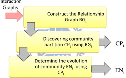
The flowchart of EPC, “relationship Extraction and community Pedigree dynamic Community miner”, shown in Fig 4-1 and consists of three phases. (1) Construct the

relationship graph RGt which is using a set of interaction graphs within observation window. (2) Use static community detection methods to discover the community partition CPt based on

the Relationship Graph produced in first step. (3) Determine the evolution of community using the community partitions.

Construct the Relationship Graph RG_t

Discovering community partition CP_tusing RG_t Determine the evolution of community EN_t using CP_t Interaction Graphs

CP

_t

EN

_t

(32)

19

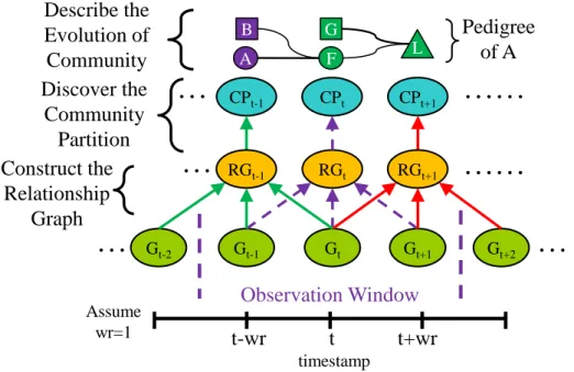
Fig 4-2 Framework of EPC, “relationship Extraction and community Pedigree dynamic Community miner”

Our framework of EPC is shown in Fig 4-2. Assuming the observation eyeshot wr = 1, tc=t, so the relationship graph RGt is constructed using interaction graphs Gt, Gt-1 and Gt+1.

Then we use static community detection method to generate the community partition CPt

based on the relationship graph RGt. While the community partitions of each timestamp have

been generated, we determine the relationship between communities at each consecutive time points using the Community Pedigree Mapping.

The graph on the top of Fig 4-2 is the pedigree of community A where a node indicates a community and an edge indicates the similarity strength between communities. The “pedigree of community A” shows all the communities which have relationship with community A. A square shape indicates the spouse community of A and the triangle shape indicates this community would be dead at next timestamp. There are 5 community spread on the timestamps {t-1, t, t+1}. The community F is similar to previous community A and B so F is the child of A and B. The community L is the child of G and F. The community B is the spouse of A and G is the spouse of F. While we want to monitor some communities to figure

F A Pedigree of A L G B G_t-2 G_t-1 G_t RG_t CP_t-1 CP_t

…

……

G_t+1 CP_t+1 G_t+2 RG_t+1 RG_t-1

……

Observation Window Assume wr=1 _t-wr _{t t+wr} timestamp

…

Discover the Community Partition Describe the Evolution of Community Construct the Relationship Graph

(33)

20

out if these communities are involved with each other, the pedigree of community would be a good way to illustrate.

We present the Relationship Extraction strategy to construct the relationship graph RGt

in chapter 4. We present current static clustering method, SHRINK [12], in chapter 5 and we propose the Community pedigree Mapping to solve the problem of evolution of communities in chapter 6.

4.2. Generating Relationship Graph?

The relationship graph RGt is constructed from interaction graphs which are most to the

current time point t. We use the observation eyeshot wr to control the observation window . For example, Assuming wr=2 and tc =3, then and the relationship graph RG3 is constructed using interaction graph G3 and those interaction graphs 2 time units before

(G1, G2) and after (G3, G4) current time tc. Then we determine the relationship strength

Wtc(u,v) between individuals u and v using the predefined normalized weight function.

Here we propose a naïve normalized weight function, normalized Equal weight function (EQL) as follows.

(2) EQL considers the interaction graph of each time point within having the same weight and makes sure the weight summation would be equal to 1. Using normalized weight function to determine the relationship strength of each pair of individuals is just like the function as follows:

(3) and is the

(34)

21

Figure 4-3 Example of determining the relationship strength

We use Fig 4-3 to illustrate how the relationship strength determined. Assuming the observation eyeshot wr equals to 2 and the interaction between individual u and v occurs at time 2, 6 and 7. The relationship strength between individual u and v at tc = 3, W3(u, v) = + + + + = (0*0.2)+ (1*0.2)+ (0*0.2)+ (0*0.2)+ (0*0.2) =0.2 . Using the same

process we calculate W4(u,v) = 0.4, W5(u,v) = 0.4 .

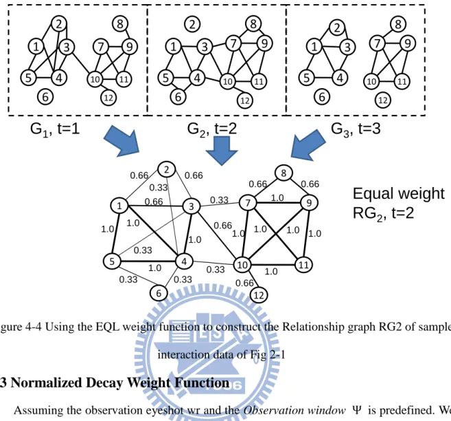
Using Eq 3 to determine the relationship graph RG2 of Fig 2-1 and the RG2 is shown on

the bottom of Fig 4-4. A node indicates an individual and the edge weight W2(u, v) indicates

the relationship strength between individuals u and v.

0.200 0.200 0.200 0.200 0.200 0 0.05 0.1 0.15 0.2 0.25 tc-2 tc-1 tc tc+1 tc+2 w ei gh t time point

Equali wieght function (EQL)

1 2 3 4 5 6

7 W

₃

(u,v)=0.2

tc-2 tc=3 tc+2

W

4

(u,v)=0.4

tc-2 tc=4 tc+2

e(u,v)

time point

(35)

22

Figure 4-4 Using the EQL weight function to construct the Relationship graph RG2 of sample interaction data of Fig 2-1

4.3 Normalized Decay Weight Function

Assuming the observation eyeshot wr and the Observation window is predefined. We propose three Normalized Decay weight functions:

Linear Decay weight function (LIN):

(4)

Wave Decay weight function:

(5)

Exponential Decay weight function:

(6)

G

₁

, t=1 G

₂

, t=2 G

₃

, t=3

Equal weight

RG

₂

, t=2

7 5 1 4 3 2 6 8 9 10 11 12 0.66 0.66 0.33 1.0 0.66 1.0 1.0 0.33 1.0 0.33 0.33 0.33 0.33 0.66 0.66 0.66 1.0 1.0 1.0 1.0 1.0 1.0 0.66 7 5 1 4 3 2 6 8 9 10 11 12 7 5 1 4 3 2 6 8 9 10 11 12 7 5 1 4 3 2 6 8 9 10 11 12

(36)

23

Fig 4-5 Normalized Decay Weight Function (wr=2)

The is based on linear decay and the weight distribution is shown in the curve (LIN) in Fig 4-5. Using to calculate the relationship strength is the same as the example in section 4-2. We multiply the weight NL(t,tc) with the interaction occurring in and sum

all the values.

The is based on the sine function of trigonometric functions to produce the relationship graph. The weight distribution is shown in the curve (WAVE) in Fig 4-5.

The is based on the approach of exponential decay function. If the weight decreases at a rate proportional to its value, it is called exponential decay [11]. The processes can be modeled by the following differential equation.

(7)

The decay constant controls the decay rate of the exponential decay and we use

Observation

Window

(37)

24

in our work. The weight distribution is shown in curve (EXP) in Fig 4-5.

For each normalized decay weight distribution, if there are some interactions whose time point is out of the Observation Window, the weight is assigned zero. Note that exponential decay weight distribution the weight of time point out of the observation window is non-zero but we simply assume the weight is zero.

4.4 Discussion of Relationship Extraction Strategy

In real world, the relationship between individuals could decay over time and the interaction at each time point within should be considered an energy which increases the

relationship strength between individuals. So we presume each interaction has the same lifetime equal to the size of observation window. Then the lifetime of each interaction would

be extended from 1 to the size of observation window. This property could overcome the weakness that there is no relationship between individuals while no interactions occur.

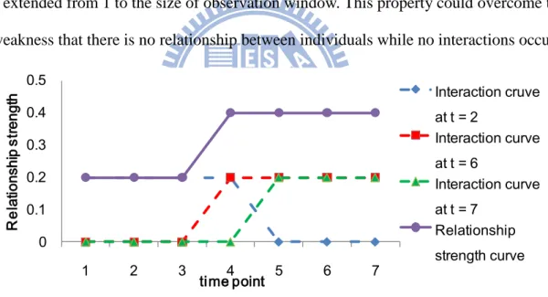
Fig 4-6. Relationship strength curve between u and v by extraction from the interaction data of Fig 4-2 based on Normalized Equal Weight Function (wr=2)

Fig 4-6 shows the evolution of relationship strength of individual u and v in the interaction data of Fig 4-3 using normalized equal weight function. The dotted line implies the interaction occurring at time points 2, 6 and 7. The interactions at all time points have the same lifetime equal to the size of observation window . The solid line sums up the curves of all interactions and represent the relationship strength of individual u and v over time.

0 0.1 0.2 0.3 0.4 0.5 1 2 3 4 5 6 7 R el at io nsh ip s tre ng th time point Interaction cruve at t = 2 Interaction curve at t = 6 Interaction curve at t = 7 Relationship strength curve

(38)

25

However, the solid line in Fig 4-6 which shows the relationship curve is higher at time t=4, 5, 6 and 7. The relationship strength curve does not match any interaction data occurred and this curve does not have the property of dynamics.

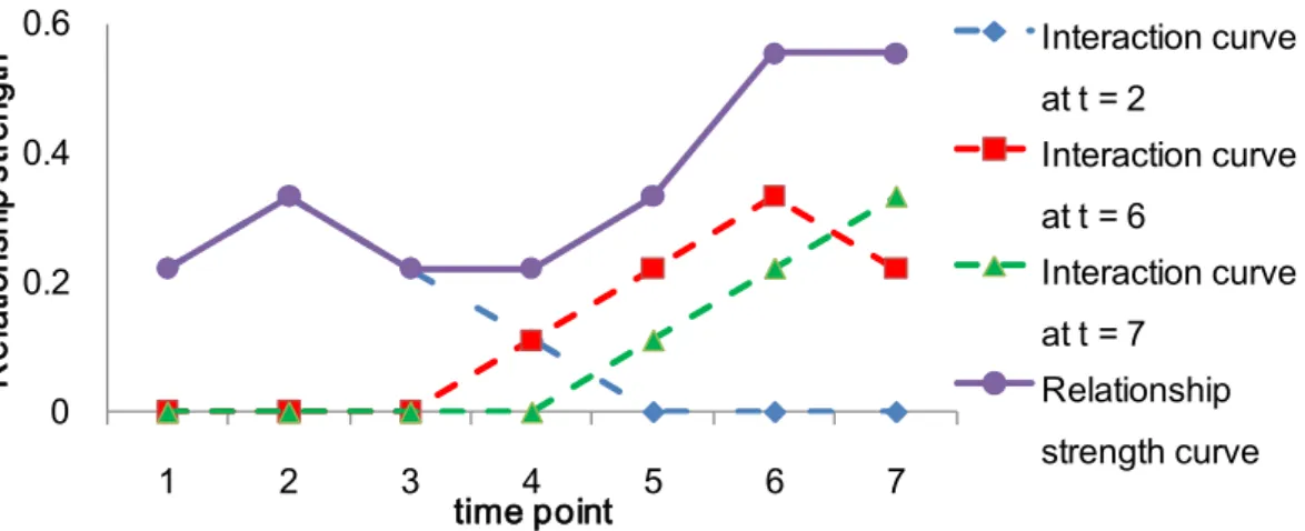
Fig 4-7. The Relationship strength curve of the interaction data of Fig4-2 based on Normalized Linear Decay Weight function (wr=2)

We change the equal weight function to the linear decay weight function and the Relationship strength curve is shown in Fig 4-7. The solid curve in Fig 4-7 indicates the relationship strength of individuals and the curve is high at t=2, 5, 6, 7 and the solid curve matches with the timestamps interaction occurred. The difference between Fig 4-6 and Fig 4-7 is that the relationship strength curve in Fig 4-7 demonstrates more dynamic property than that in Fig 4-6 so the normalized decay weight function would be more realistic than equal weight function. 0 0.2 0.4 0.6 1 2 3 4 5 6 7 R el at io nsh ip s tre ng th time point Interaction curve at t = 2 Interaction curve at t = 6 Interaction curve at t = 7 Relationship strength curve

(39)

26

Chapter 5 Current Static Community Detection methods

After generating relationship graphs at each time point, we choose static community methods for discovering the community partition at each timestamp. Although many of studies have focused on community detection on static networks, not every method is suitable for relationship graph. Two issues need to be considered about: (1) Discovering communities using the weighted graph (relationship graph). (2) Detecting the noisy vertices whose relationship strength is too low to belong to any community. The SHRINK algorithm [12] overcomes the problem of parameters pre-definition, such as minimum similarity threshold ( ) and minimum core size ( ), in density-based clustering algorithms and the predefined number

of clusters in partitioning-based clustering algorithm. Through their experiment, SHRINK is an efficient, parameter free and high accuracy algorithm while comparing with other algorithm [18, 19]. So we choose SHRINK as our clustering algorithm. For comparison, we also use the greedy density-based clustering method (GSCAN) used in PD-Greedy [5, 21].

In section 5.1 we represent the detailed definition of GSCAN and section 5.2 represents the definition of SHRINK. Section 5.3 illustrates the quality measurement of community partition. Section 5.4 describes the detail algorithm of SHRINK algorithm and the algorithm of GSCAN is represented in section 5-5.

5.1 GSCAN

In this chapter we present the definition of GSCAN and related notation. Let (V, E, ) be a weighted undirected network where is the weight set of edge set E, GSCAN uses the structure similarity as similarity measure and the related definition is as follows:

Definition 7 [5]. (Neighborhood)

Given G= (V, E, ), for a node u and the adjacent nodes of are neighbors of ( ). i.e.: .

(40)

27

Let G= (V, E, ) be a weighted undirected network. The structural similarity between two adjacent nodes and is defined as below:

(8) where indicate the weight of

GSCAN applies a minimum similarity threshold ε to the computed structural similarity when assigning cluster membership as formalized in the following ε -Neighborhood definition:

Definition 9[5]. (ε -Neighborhood)

For a node V, the ε -Neighborhood of a node is defined by

When a vertex shares structural similarity with enough neighbors, it becomes a seed for a cluster. Such a vertex is called a core node, Core nodes are a special class of vertices that have a minimum limit of neighbors with a structural similarity that exceeds the threshold ε [21].

Definition 10[5]. (Core node)

A node V is called a core node w.r.t. Definition 11[5]. (Directly reachable)

A node x V is directly reachable from a node V w.r.t. if (1) node is core node. (2) x .

Definition 12[5]. (Reachable)

A node V is reachable from a node V w.r.t. if there is a chain of nodes such that is directly reachable from (i < j) w.r.t. .

Definition 13[5]. (Connected)

A node V is connected to a node u V w.r.t. if there is a node x V such that both and u are reachable from x w.r.t. .

(41)

28 Definition 14[5] (Connected cluster)

A non-empty subset S V is called a connected cluster w.r.t. if S satisfies the following two conditions:

(1) Connectivity: S, v is connected to w w.r.t .

(2) Maximality: V, if v S and is reachable from w.r.t , then S.

Using the above definition, a structure-connected cluster with respect to ε , μ is uniquely determined by any cores of this cluster.

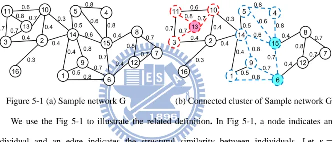
Figure 5-1 (a) Sample network G (b) Connected cluster of Sample network G We use the Fig 5-1 to illustrate the related definition. In Fig 5-1, a node indicates an individual and an edge indicates the structural similarity between individuals. Let , we could evaluate the Core nodes as node 13, node 15 and node 6. The node 10 is Directly reachable from node 13 due to that node 13 is a core node and . The node 4 is Reachable from node 6 due to the Directly reachable chain (node 6, node 15, node4). Based on the definition of Connected cluster, there are two clusters, {3, 10, 11, 13} and {1, 4, 5, 6, 9, 14, 15}.

5.2 SHRINK

In this section we introduce SHRINK and related notation. For structural similarity measure, SHRINK uses the same cosine similarity as GSCAN and the related definition is as follows:

Definition 15[12]. (Dense Pair) 11 12 13 14 15 2 3 10 7 8 6 1 9 5 ₄ 0.7 0.4 0.7 0.4 0.4 0.8 0.7 0.8 0.6 0.7 0.3 0.7 0.7 0.8 0.8 0.7 0.5 0.8 0.4 0.6 0.8 0.5 0.6 16 0.3 _0.4 0.4 11 12 13 14 15 2 3 10 7 8 6 1 9 5 ₄ 0.7 0.4 0.7 0.4 0.4 0.8 0.7 0.8 0.6 0.7 0.3 0.7 0.7 0.8 0.8 0.7 0.5 0.8 0.4 0.6 0.8 0.5 0.6 16 0.3 _0.4 0.4

(42)

29

Given a network G(V,E), If is the largest similarity between nodes and their adjacent neighbor nodes. i.e.: then is called a Dense Pair in G, denoted by , where is the largest similarity between nodes and their adjacent neighbor

nodes.

Definition 16[12]. (Micro-community)

Given a network G=(V,E), MC(a)= is a connected sub-graph which is represented by node a in network G. MC(a) is a local Micro-community if and only if

(1)

(2) (3)

where represents the largest similarity between nodes and their adjacent neighbor nodes.

We use the Fig 5-1(a) to illustrate the Dense Pair and Micro-Community. All the Dense

Pair within the Fig 5-1(a) are shown in Fig 5-2. The dot line nodes and dot line edges indicate

that these nodes are Dense Pair and could be grouped into a Micro-Community.

Figure 5-2 All Dense Pairs within the sample network G in Fig 5-1(a) Definition 17[12]. (Super-network)

Given a network G=(V, E, ), is a community partition of the node set V and , the sub-network MCi=(Vi, Ei) induced by the node set Vi is a local

11 12 13 14 15 2 3 10 7 8 6 1 9 5 ₄ 0.7 0.4 0.7 0.4 0.4 0.8 0.7 0.8 0.6 0.7 0.3 0.7 0.7 0.8 0.8 0.7 0.5 0.8 0.4 0.6 0.8 0.5 0.6 16 0.3 _0.4 0.4

(43)

30

Micro-community in G. Define and

; then is called a Super-network of G.

Especially, the algorithm not only discovers all the communities but also the hubs and outliers in the network. A hub is called an overlap community and a hub plays a special role in many real networks such as search engines of web page network and the communication center of protein. An outlier does not belong to any communities because the similarities between it and other nodes are too small. This algorithm does not partition all the nodes into communities and this property is just perfect for our requirement.

5.3 Measurement of Partitioning Quality

Although several well-known quality measures such as normalized cut [24] and modularity [18] have been proposed, the modularity is the most popular measure by far. GSCAN and SHRINK both use the same similarity based modularity function Qs [25].

(9)

Assume the community partition has k communities { , , ..., },

is the total similarity of the nodes within cluster ,

is the total similarity between the nodes in cluster and any nodes in the network, and is the total similarity between any two nodes in the network.

SHRINK is based on this quality function (Qs) and incrementally calculates the increment of the modularity quality. Given two adjacent local communities and , the modularity gain can be computed by

(10)

Where

is the summation of similarity of total edges between two communities and .

(44)

31

i.e.: , the modularity gain for merging a micro-community into a super-node can be easily computed as

(11)

SHRINK uses the modularity gain to control the shrinkage of the micro-communities. Only while the modularity gain is positive , these communities within micro-community (MC) could be merged into a super-node.

5.4 Algorithm of SHRINK

We use Fig 5-1 ~ Fig 5-5 to illustrate the key point of SHRINK. Given a simple network G as shown in Fig 5-1, nodes indicate the individuals and the weight of an edge indicates the Structural Similarity between individuals.

Each round of process of SHRINK has two phases. (1) For each node u we considered u as a micro-community MC(u), determine if each neighbor of the node x within MC(u) is the Dense pair. If x within MC(u) and a node v of the neighbors of x is Dense pair, then push v into the micro-community MC(u). The example is shown the Fig 5-3(a) and 5-4(a). The dotted lines indicate all Dense pairs found in the network G. (2) SHRINK determines the for all micro-communities {MC1, MC2, …MCk} and only while the , all the

nodes of the micro-community MCi would be merged into a super-node which contains more

than one node at next round. Fig 5-3(b) and 5-4(b) show the second process of SHRINK. Fig 5-5(a) shows the result of third round of the SHRINK process and Fig 5-5(b) shows the fourth round of the SHRINK process. Fig 5-5(b) displays that the process of SHRINK terminates of . The network shrieked from G is called Super-network as shown in Fig

5-3(a) and Fig 5-4(a). Fig 5-5(b) shows the final result of SHRINK and there is a hub (node 2) and an outlier (node16).

(45)

32

Fig 5-3 Round 1(a): Find all Dense pairs in G (b)Δ Q>0, Shrink

Fig 5-4 Round 2(a): Find all Dense pairs in G (b)Δ Q>0, Shrink

Fig 5-5 (a): Round 3 shrink becauseΔ Q>0 (b) Round 4 no-shrink becauseΔ Q<0

Algorithm1 : SHRINK[12] Input: weighted networks G = (V, E)

Output: Set of clusters CP = {C1, C2, …, Ck}; Set of hubs and outliers N; 1: CP ;

2: while true do

3: //Phase 1: Detect the all Dense Pairs of G 4: Micro-community MC ( ) ← {v}; 5: for each unclassified do 6: temp community C(v) ; 7: Classify ; Queue q; q.insert(v) ; 8: ; 9: While q.empty() true do

10: u q.pop(); 11: if u=v max{ }= 12: C(v) ← C(v) {u} ; 13: for each w 14: if = 11 12 13 14 15 2 3 10 7 8 6 1 9 5 ₄ 0.7 0.4 0.7 0.4 0.4 0.8 0.7 0.8 0.6 0.7 0.3 0.7 0.7 0.8 0.8 0.7 0.5 0.8 0.4 0.6 0.8 0.5 0.6 16 0.3 _0.4 0.4 11,13 14,9 2 3 10 7 8,12 1,6 5,4,15 0.4 0.7 0.4 0.4 0.7 0.7 0.3 0.7 0.6 16 0.3 0.4 0.4 11,13 14,9 2 3 10 7 8,12 1,6 5,4,15 0.4 0.7 0.4 0.4 0.7 0.7 0.3 0.7 0.6 16 0.3 0.4 0.4 11,13, 3,10 14,9, 1,6 2 8,12, 7 5,4,15 0.4 0.3 _0.6 16 0.3 0.4 0.4 0.4 11,13, 3,10 2 8,12, 7 14,9,1,6 5,4,15 0.3 16 0.3 0.4 0.4 0.4 11,13, 3,10 2 8,12, 7 14,9,1,6 5,4,15 0.3 16 0.3 0.4 0.4 0.4 Hub Outlier

(46)

33 15: q.insert (w) ; 16: end 17: end 18: end 19: end 20: MC ← MC C(v) 21: end

22: //Phase 2.2: Shrink micro-community 23: 24: for each C MC do 25: if then 26: CP ← (CP ) ; 27: ← + ; 28: end 29: end 29: if then 30: break; 31: end 32: end 33: N ← 34: for each C CP do 35: if |C|=1 36: CP ← CP C ; 37: N ← N C ; 38: end 39: end 40: return CP, N ;

Figure 5-6 Algorithm of SHRINK

5.5 Algorithm of GSCAN

In this section, we describe the algorithm GSCAN. GSCAN is extended from SCAN [21] and combines with greedy heuristic setting of ε . SCAN performs one pass scan on each node of a network and finds all structure connected clusters for a given parameter setting. The pseudo code of the algorithm SCAN is presented in Fig 5-7. Given a weighted undirected graph G (V, E), at the beginning all nodes are labeled as unclassified. For each node that is not yet classified, SCAN checks whether this node is a core node. If the node is a core, a new cluster is expanded from this node. Otherwise, the vertex is labeled as a non-member.

GSCAN use greedy heuristic setting of ε to optimize the modularity score Q of clustering result. GSCAN adjusts the ε with change of modularity score Q and decreases or increasesε until Q reaching the local maximum modularity [5].

(47)

34 Algorithm2 : SCAN [21]

Input: weighted networks G = (V, E), ε , μ

Output: Set of clusters CP = {C1, C2, …, Ck} , modularity score Q . 1: // all nodes in V are labeled as unclassified;

2: CP ← ;

3: for each unclassified node v V do 4: // STEP 1. check whether v is a core; 5: if COREε ,μ (v) then

6: // STEP 1.1. if v is a core node, a new cluster is expanded; 7: set C ← ;

8: insert all into queue Q; 9: while Q ≠ 0 do

10: y = first vertex in Q;

11: R = {x V | DirREACHε ,μ (y, x)}; 12: for each x R do

13: if x is unclassified or non-member then 14: C ←C x;

15: end

16: if x is unclassified then 17: insert x into queue Q; 18: end 19: end 20: remove y from Q; 21: end 22: CP ←CP C; 23: end 24: end

25: // 1.2 determine the modularity score of CP; 26: Q = (CP);

27: return CP , Q

Figure 5-7 Algorithm of SCAN

GSCAN chooses a median of similarity values of the sample nodes picked from V and the sampling rate is only about 5~10%. GSCAN increases or decreases the by a unit = 0.01 or 0.02 and maintains two kinds of heaps: (1) max heap Hmax for edges having similarity

below seedε ; and (2) min heap Hmin for edges having similarity above seedε . Hmax and

Hmin are built during the initial clustering. After finding the initial clusters CP and calculating its modularity Qmid, GSCAN calculates two additional modularity values, Qhigh and Qlow. Here,

Qhigh is calculated from CP with the edges having similarity of range [seedε , seedε + ] in

Hmin, and Qlow calculated from CP except the edges having similarity of range [seedε - ,

seedε ] in Hmax. If Qhigh is the highest among Qhigh, Qmid, and Qlow, GSCAN increases the

運用關係萃取策略於動態社群探勘之研究

國

立

交

通

大

學

資訊科學與工程研究所

碩

士

論

文

運用關係萃取策略於動態社群探勘之研究

Dynamic Community Detection via Relationship

Extraction Strategy and Community Pedigree Mapping

研 究 生：彭誠毅

指導教授：李素瑛 教授

運用關係萃取策略於動態社群探勘之研究

Dynamic Community Detection via Relationship Extraction Strategy and

Community Pedigree Mapping

研 究 生：彭誠毅 Student：Cheng-Yi Peng

指導教授：李素瑛 Advisor：Suh-Yin Lee

國 立 交 通 大 學

資 訊 科 學 與 工 程 研 究 所

碩 士 論 文

運用關係萃取策略於動態社群探勘之研究

國立交通大學資訊科學與工程研究所

摘要

Dynamic Community Detection via Relationship Extraction

Strategy and Community Pedigree Mapping

Cheng Yi Peng Suh-Yin Lee

Institute of Computer Science and Information Engineering

National Chiao-Tung University

Abstract

show that EPC not only

significantly outperforms the prior studies in accuracy but also possesses

graceful scalability and smoothness.

Index terms: dynamic community, relationship extraction, decay weight

ACKNOWLEDGEMENT

Table of contents

List of Figures

List of Tables

Chapter 1.

Introduction

Chapter2

Related Works and Motivation

2.1 Community Detection in Static Graphs

2.2 Community Detection in Dynamic Graphs

2.2.1 Two-Stage Approach

G1, t=1 G2, t=2 G3, t=3

t F

A

B

C

t-1

G

H

D

E

I

J

2.2.2 The approach of Evolutionary Clustering

Temporal Smoothness

G

G

G

CP

CP

CP

…

…

Interaction

Graph

Evolutionary

Community

Partition

v2

v1

v5

v4

研究生：彭誠毅

指導教授：李素瑛教授

研究生：彭誠毅 Student：Cheng-Yi Peng

國立交通大學

資訊科學與工程研究所

碩士論文