DETERMINATION OF 3D HUMAN-BODY POSTURES FROM A SINGLE VIEW

Determination of 3D Human Body Postures from a

Single View

HSI-JIAN LEE AND ZEN CHEN

The Institute of Computer Engineering, National Chiao-Tung University, Hsinchy Taiwan, Republic of China

Received February 8,1984; revised September 24,1984; accepted November 13,1984 In this paper a method is proposed to recover and interpret the 3D body structures of a person from a single view, provided that (1) at least six feature points on the head and a set of body joints are available on the image plane, and (2) the geometry of head and lengths of body segments formed by joints are known. First of all, the feature points on the head in the head-centered coordinate system and their image projections are used to determine a transfor- mation matrix. Then, the camera position and orientations are extracted from the matrix. Finally, the 3D coordinates of the head points expressed in the camera-centered coordinate system are obtained. Starting from the coordinates of the neck, which is a head feature point, the 3D coordinates of other joints one-by-one are determined under the assumption of the fixed lengths of the body segments. A binary interpretation tree is used to represent the 2”-’ possible body structures, if a human body has n joints. To determine the final feasible body structures, physical and motion constraints are used to prune the interpretation tree. Formulas and rules required for the tree pruning are formulated. Experiments are used to illustrate the pruning powers of these constraints. In the two cases of input data chosen, a unique or nearly unique solution of the body structure is obtained. e 1985 Academic PI~SS, IIIC.

1. INTRODUCTION

Computer vision for recovery of 3D object structure has received increasing attention recently. It is mainly because of numerous potential applications in the industry, military, and others. There are various methods for determining 3D object structure. They are the stereo vision [l], shape from shading [2, 31, shape from texture 14, 51, shape from contour [6], and structure from motion [7-lo], to name a few. The applicability of these methods depends on many factors such as

(a) the imagery type, e.g., an array of range data or gray values, (b) the type of illumination, e.g., structured light or general light, (c) the number of views and the possible relations between the views, (d) the object type, e.g., rigid, jointed, or amorphous,

(e) a priori information about the object, e.g., structure model or material property.

Among these factors, the first two factors are important as far as image segmenta- tion is concerned; the last three. factors are valuable for the determination of the spatial positions of object points and the object connectivity structure. We shall consider only the rigid and jointed objects.

148 0736189X/85 $3.00

Copyri&t 0 1985 by Academic Press. Inc. All rights of reproduction in any form reserved.

3D HUMAN BODY POSTURES 149

For a rigid object it generally requires more than a single view for any meaningful 3D recovery of object structure. We shall discuss the 3D recovery methods based on one or multiple views obtained via a single camera. Roberts ill] did the pioneer work on machine perception of 3D objects based on a formulation in terms of the homogeneous coordinate system. In this framework Rogers and Adams [12] showed that at least six object points were needed to determine their 3D coordinates from a single 2D view. Ullman [7] used four points of the object over three views to obtain the object structure. Roach and Aggarwal[8] studied the recovery method based on five noncoplanar points over two views under perspective projection. A general formulation for the relationship between the numbers of points and views was given by Meiri [9]. In the above methods the point correspondence between two views is assumed known. The methods for solving the point correspondence problem were studied by Rashid [lo], and Barnard and Thompson [13].

In the determination of the 3D structure of a jointed object, Rashid [lo, 141 proposed a three-stage approach, i.e., correspondence, object separation, and de- termination of subparts. He used a minimum spanning tree (MST) approach in a four-tuple space formed by the projected position and projected velocity of the points on the 2D image plane. In this way he derived the connectivity relationships between object points and broke the MST to obtain subparts. On the other hand, O’Rourke and Badler [15, 161 advocated a model-based system for the human motion interpretation. They represented a human body model by 24 segments and 25 joints. The flesh of each segment is in turn characterized by a set of spheres. The system is structured as a closed loop between a high level component, i.e., the prediction, and a low level component, i.e., image analysis. The input of the image analysis component is a list of 3D regions where various body features are predicted to appear; the actual location of a feature is searched within the area predicted for that feature. The 2D location boxes of features extracted are fed back through a constraint network to refine the 3D best-guess rectangular boxes of features. The constraints checked include distance measures, angle limits, and collision detections. Webb and Aggarwal [17] used a fixed axis assumption to determine the 3D structure of a jointed object from several views under the parallel projection. Namely, a feature point, with respect to another reference feature point on the same rigid part, will form a circle in the 3D space, when it moves; the parallel projection of a circle on the image plane is an ellipse. Given the point correspondences in the multiple views, one can then group those points as being on the same rigid part, if their relative positions with respect to a certain reference point can be fitted by individual ellipses.

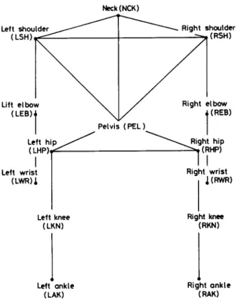
In this paper we shall consider the recovery of a human body from a different viewpoint. As mentioned previously, a single 2D view is not sufficient for a general recovery. Here we shall assume the physical structure of the human body under study is known. The human body will be represented as a stick figure. The stick figure indicates the connectivity of body segments and is found popular in the field of human movement analysis, as reported by Badler and Smoliar [18]. We shall adopt a stick figure model containing 14 joints and 17 segments, as shown in Fig. 1. Here the torso, formed by the neck, right shoulder, left shoulder and pelvis, is assumed rigid; so is the hip part, formed by the pelvis, right hip, and left hip. On top of the neck, there is the head which is characterized by six or more feature points, e.g., two eyes, two ears, one nose tip, and the neck. The lengths of all 17 segments

Neck (NCK)

Lift elbow Right elbow

Left wrisi Right .wrist

(LwR)A 1 mm

Left knee (LKN)

Right knee (RKN)

FIG. 1. The stick-figure human body model containing 14 joints and 17 segments. The head is not shown.

and the 3D positions of the feature points on the head are assumed known. In our study, we also assume that the head points and the 14 joints are already identified on the image plane beforehand.

To demonstrate our theory we shall use the synthetic input data generated by Cutting [19] with minor modifications. The Cutting’s synthetic data is also used by Rashid [lo], called moving light displays. Similar displays of point lights or bright regions were used by Johansson [20], Webb and Aggarwal [17], and O’Rourke and Badler [Ml. Our work is similar to Herman’s work [23] and O’Rourke and Badler’s work [16] in the sense that they all study legal body postures or movement. However, the input data used by Herman is specified in terms of the line segments of body parts and angles at joints on the image plane. And the input data used by O’Rourke and Badler is essentially a set of 3D predicted regions containing the feature points. Our input data is a set of 2D projected coordinates of the joints. On the other hand, the outputs of the previous two works are about semantic descriptions of the human body movement; our output is a set of 3D body structures which represent possible body movements.

Section 2 describes a recovery process for obtaining the human body configura- tions. Section 3 gives a representation scheme, i.e., a binary interpretation tree, which stores all possible body configurations. Then we introduce the physical constraints and motion constraints for removing infeasible body cotigurations.

3D HUMAN BODY POSTURES 151 Section 4 is on the experimental results and discussions. Section 5 contains a summary.

2. RECOVERY PROCESS

2.1. Relationship between Rigid Object Structure and Camera Model

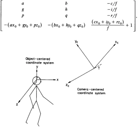
A person is assumed to be specified in a right-handed object-centered coordinate system, while a camera is specified in a left-handed camera-centered coordinate system, as shown in Fig. 2. The object-centered coordinate system is defined on the head of a person, so it is also called a head-centered coordinate system.

A point (x, y, z) in the head-centered coordinate system and its perspective projection (x’, y ‘) on an image plane can be represented by (x, y, z, 1) and (X, Y, H), respectively, in a homogeneous coordinate system. Here, x’ is equal to X/H and y’ is equal to Y/H. We can relate these two coordinates by the following equation [ll, 121:

b,

Y,

z, O*[U = (x y, HI,

(1)

where [T] denotes a transformation matrix.

The matrix [T] can be readily shown to be the product of a translation matrix, a rotation matrix, a conversion matrix from the right-handed coordinate system to the left-handed coordinate system, and a perspective projection matrix. In matrix notation, [T] can be represented as

a b

_{- c/f}

g

h

_{- i/f}

P 4

- r/f

-(ax0 + m + pz,) -(bx, + hy, + qzo) (cxo + iyO + rzO)

f

+1 Object-centered coordinate system Yc _xc Y 3’ ZC Camera -centered coordinate system

where the matrix

a b c [RI=

1 1

g h i

P 4 r

is an orthonormal rotation matrix; the vector (x,, yO, z,,) is the translation vector between the origins of the two coordinate systems; and f is the lens-to-image-plane distance.

We rewrite the matrix [T] as

By using this notation and Eq. (l), we can obtain the following two equations: t,,x + t,,y + t,,z + t,, - f14XX’ - t,,yx’ - t34zX’ - t&$x’ = 0

*12x + *22y + *32z + *42 - t,,xy’ - t2ayy’ - t,,zy’ - fey ‘=O

(2) .

Here we have two equations with 12 unknown variables, { tmn}, m = 1,2,3,4; n = 1,2,4. We need six independent points to solve for {t,,}. These 12 equations can be rearranged in a compact form, i.e.,

[A]*W = 0, (3)

where JV denot= a dumn vector (*11, *12, t14, *21, *22, t24, *jl, tj2, *34, *41, 142, td’;

with the symbol ’ being the transpose operator, and [A] is a 12 X 12 matrix.

From Eq. (3), if [S] is a solution for matrix [T], then k*[S] is also a solution for any scalar k. Here the matrix [S] is represented as follows:

Sl $2 s3 [s] = ;: ;‘, ;; .

[ 1

-50 311 812

The relationships between the elements in matrix [T] and matrix [S] are given by

(a9 g, p) = k*(s1,S4,

ST) = (h, tZ13

*,,)

(b, hq) = k*b2, wg) = (*n, *22,

t,,)

-(c,i,r)/f=

k*(S3,Sg,Sg)

=

(*14,t24,*34).

(4

From any of the first two equations listed above, we can solve k since the column vectors (a, g, p >‘, (b, h, q)‘, and (c, i, r >’ in the matrix [T] are orthonormal vectors.

3D HUMAN BODY POSTURES 153 Taking an example, from the first equation we obtain

k2 = l/( s; + s; + s;).

Therefore, we can find the solution for the rotation matrix [RI. We can also find the value of

f

from the third equation.

As soon as the matrix [S] is normalized, the camera position (x,,, ya, z,,) can be solved by equating the fourth rows of the matrices [S] and [T]. The solution can be represented by the following matrix form

We choose six feature points on the head to determine the camera position. The six feature points chosen are neck, nose, right eye, left eye, right ear, and left ear. In practice, we can choose more than six feature points on the head and use the least-squares method to obtain a reliable result.

2.2. Detemination of Jointed Object Structure

Based on the stick-figure human model, we can group the joints according to the lengths of the paths constructed from the neck to them. The joint which is closer to the neck in a segment is called the starting joint, and the other is called the ending joint. We group all joints into four classes:

Class (a) = {right shoulder, left shoulder, pelvis}, Class (b) = {right elbow, left elbow, right hip, left hip}, Class (c) = {right wrist, left wrist, right knee, left knee}, Class (d) = {right ankle, left ankle}.

Starting from the neck, we can tlnd the coordinates of those joints in Class (a), namely, right shoulder, left shoulder, and pelvis. Next, we can find the coordinates of the joints in Class (b) and so on.

When the coordinates of the starting joint (xs, y,, zs) of a rigid segment are known, the coordinates of the ending joint (xe, y,, ze) can be found in the following manner:

The coordinates of the ending joint (x,, y,, z,) in the camera-centered coordinate system and its projection (xi, $) are related by

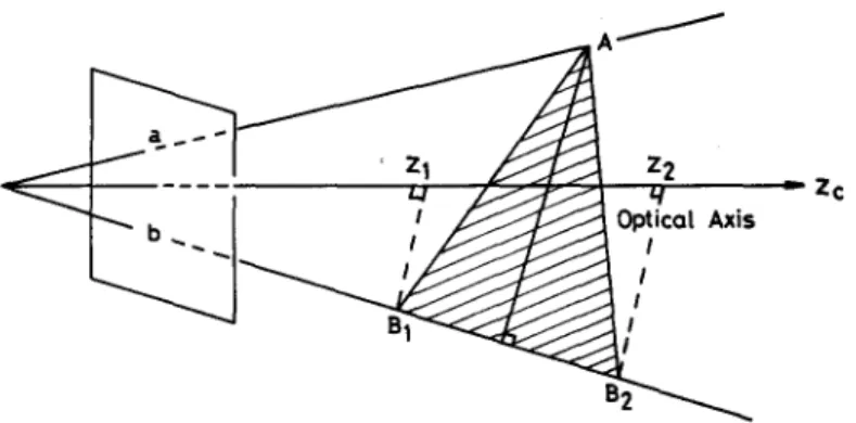
FIG. 3. Two possible solutions for an ending joint.

where the number k is a scalar factor. Hence, x, = x:k, Y, = y.3,

z, = f*(k - 1). _(6b)

The length, I,, between two joints (x,, y,, zS) and (xe, ye, z,) can be expressed as 1: = (xs - xJ2 +(y, -ye)* +(z, - z,)*.

₍₇₎

By assumption, the length of the rigid segment is known, so we can express Eq. (7) in terms of k. There are two solutions for k except for the degenerate case. Therefore, there exist two possible 3D coordinates for each ending joint. This will be called the joint positional ambiguity. Fig. 3 illustrates the two possible solutions.

3. DERIVATION OF BODY CONFIGURATIONS 3.1. Interpretation Tree

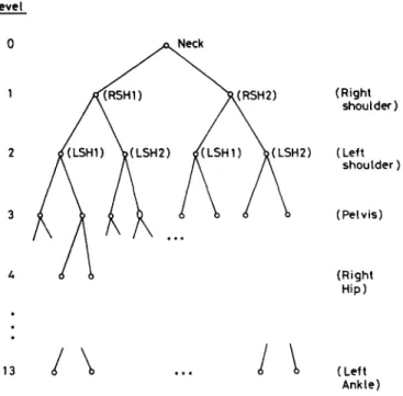
In order to represent all possible combinations of the coordinates of joints, we define a binary interpretation tree to represent the solution space. The tree consists of n levels, where n denotes the total number of joints including the neck (n = 14, in our case). The arrangement of these levels is according to the order of the lengths of paths defined before. For the joints in the same class, the order is an arbitrary permutation of joints in that class. Fig. 4 shows a partial view of this tree.

In this tree each node has two successors which correspond to the two candidate solutions obtained in the process mentioned above. There are 2’ possible nodes at level i, 0 I i s 13. A path from level 0 to level 13 define a possible body configuration or posture. Therefore, there are totally 213 = 8196 body configurations in the tree. Each body configuration stands for a body structure.

Among the 213 body configurations, there are usually quite a few configurations which are not feasible from the viewpoint of physical constraints. Here the physical constraints are mainly due to (a) the limits of angular movements at various joints, (b) the inter-distances between joints of rigid body parts, and (c) the collision-free

3D HUMAN BODY POSTURES 155 level (Right shoulder) (Left shoulder ) (Pelvis) 1 d b (Right Hip) . .*. (Left Ankle)

FIG. 4. A partial binary interpretation tree.

requirement of body parts. In addition to the physical constraints which are independent of the specific motion that the person is making, we can further reject certain configurations based on the motion constraints. To apply the physical and motion constraints mentioned above, we need to define all the formulas required. To this end, we shall specify a common coordinate system to be used throughout the analysis of body configurations. Let the origin of a right-handed coordinate system be located at the neck joint and the three coordinate axes be parallel to the following vectors:

y = the vector from the neck to the pelvis,

z = the vector from the right shoulder to the left shoulder, x = the cross product of y and z.

3.2. Tree Pruning by Physical Constraints A. Angle Constraints

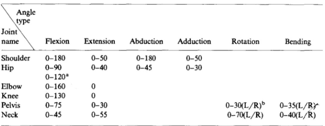
Now consider the first type of physical constraints, i.e., angle constraints. There are at least four different categories of angles associated with the human body joints. These are (a) flexion/extension, (b) abduction/adduction, (c) rotation, and (d) bending. The allowable ranges of these angles vary slightly from person to person. The general ranges of these angles can be found in the field of kinesiology. A typical set of angle values is given in Table 1 [21]. In the following we shall define the angle formulas at various joints.

TABLE 1 Angle Constraints at Joints

Flexion Extension Abduction Adduction Rotation Bending

Shoulder O-180 O-50 O-180 O-50

Hip O-90 O-40 o-45 O-30

O-120”

Elbow O-160 0

Knee O-130 0

Pelvis o-75 O-30 O-30(L/R)b o-35(L/rQ

Neck o-45 o-55 0-7O(L/R) @w-/k)

“The range applies when flexion at knee is allowed bL/R means left/right.

(i) At the shoulder/hip joint. Let the upper arm, either right or left, be specified by a vector u from the shoulder to the elbow. Assume that the projection vectors of u onto the xy plane and yz plane are II,,~ and uY,=, respectively. Define

0 = the angle from the y axis vector to the projected vector u,, y with a value from 0” to HO”,

+ = the angle f rom the y axis vector to the projected vector u,,= with a value from 0’ to 180”.

Then the angle 8 is the flexion angle at the shoulder joint if B is a clockwise angle in the x, y coordinate system; otherwise 8 is the extension angle. Similarly, 9 is the abduction angle at the right (left) shoulder joint, when $J is a clockwise (counter- clockwise) angle in the y, z coordinate system; otherwise $J is the adduction angle. By analogy, the flexion/extension angle and abduction/adduction angle at the hip joint can be derived, too.

(ii) At the elbow/knee joint. Next, we shall consider the flexion/extension angle at the right or left elbow joint. Define

v = the vector from the elbow to the wrist, w = the cross product of v and u, and

\c, = the angle measured from v to u with a value from 0’ to 180’.

Then the angle # is the flexion angle at the elbow, when w has a nonnegative z component; otherwise # is the extension angle at the elbow. By the same token, the flexion/extension angle at the knee joint can be similarly defined.

(iii) At the pelvis joint. The flexion/extension angle at the pelvis is detined to be the angle formed by the torso plane and the hip plane. This is generally defined when a person moves his torso toward or away from the hip plane. Let the normal vector of the hip plane have a projected vector nX,Y on the xy plane. Also assume the angle measured from the x axis vector to the vector nX,Y is S with a value from 0” to 180". Then the angle S is the flexion angle at the pelvis joint, if 6 is a clockwise angle; otherwise 6 is the extension angle.

3D HUMAN BODY POSTURES 157 The rotation at the pelvis joint can be conceived as the relative angular motion between the two normal vectors of the torso plane and the hip plane on the zx plane. Assume the projected vector of the normal vector of the hip plane on the LX plane is denoted by nr,x. Then the angle between the x axis vector and the vector n r.x, measured on the zx plane, is the rotation angle at the pelvis joint. The rotation can be to the either side of the x axis vector.

The bending angle at the pelvis joint is defined to be the angle between the y axis vector and the projected vector, on the yz plane, of the vector constructed from the pelvis joint to the m iddle point of the line connecting the two hip joints

(iv) At the neck joint. The various angles associated with the neck joint are defined by the head plane and the torso plane in the same manners as in the cases of the pelvis joint.

B. Distance Constraints

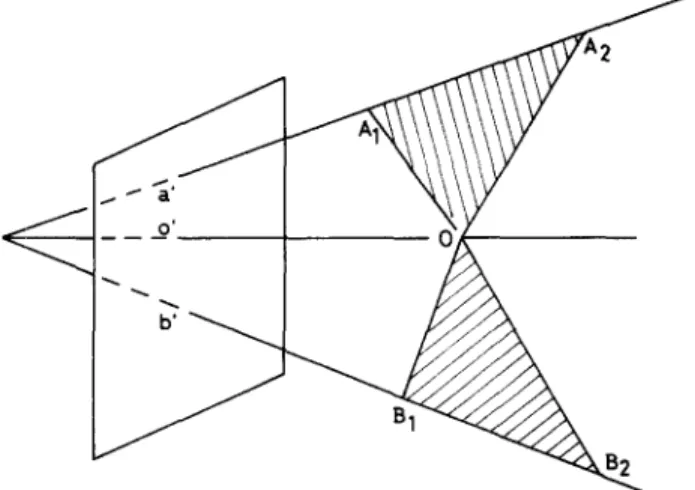
The use of distance constraints is twofold. First, they have been used to find the joint coordinates in the recovery process. Second, if a rigid part has more than two joints, the distance constraints can also be used to reduce the combinations of possible solutions of joints. Figure 5 shows the projections of three joints of a rigid part on the image plane. We take the torso as an example. Here, we assume the spatial point of the neck joint 0 is corresponding to image point 0’. Thus A,, A,, B,, and B, are the possible 3D coordinates of the two shoulders corresponding to image points a’ and b’, respectively. Given the distance between the right and the left shoulders, we can decide the correct combination from line segments A,B,, m , &&, and A,B,.

C. Collision-free Constraints

We shall check the collision conditions between body segments. Here we mainly examine whether the arm segments penetrate the torso and whether the arm and leg segments collide each other.

--

FIG. 5. The projections of 3 joints of a rigid part on the image plane. The planes OA,A, and OB,&

3.3. Tree Pruning by Motion Constraints

The human body can make a remarkably large number of different body postures. We shall assume that we are only interested in “meaningful” body postures. Simply applying the physical constraints mentioned above is not sufficient with regard to the determination of meaningful human motion. One way to obtain the meaningful body postures is to make a postulate of the body posture. In other words, we try to infer a set of body postures based on a certain “motion model.” The more a priori knowledge about the human motion is available, the better the chance for us to understand the meaning of the body postures is. In this study, we shall consider the motion model of walking. Therefore, we use a set of rules to verify the correctness of body postures under the assumption of a walking model. The rules can range from general assertions to stringent assertions. The pruning power associated with these rules certainly depends on the specificity of the rules. Two fairly general rules of the walking model are given below.

Rule 1. The two arms cannot be both in front of or behind the torso simulta- neously. The same restriction also holds for the two legs.

Rule 2. The arm and the leg which are on the same side of the body cannot swing forward or backward at the same time.

Next, we shall consider the cooperative movement of the elbow and the shoulder. In general, when these two joints both move, they will swing forward or backward at the same time; otherwise due to the physical structure of the shoulder and the elbow the two swings in opposite directions will result in something like a dislocated arm. By the same token the hip joint and the knee joint must swing in the same direction. Here the hyperplane indicating the body plane without swing can be derived by the line segment from the neck to the pelvis and the normal vector to the head plane. The above is summarized in Rule 3.

Rule 3. When both the shoulder joint and the elbow joint of either arm swing, they must swing in a cooperative manner. The same holds for the hip joint and the knee joint of either leg.

Two additional, stringent rules of the walking model are listed below.

Rule 4. The trajectory plane on which the arm or leg swings is generally parallel to the moving direction.

Rule 5. At any time instant of walking, there is at most one knee having a flexion angle. Moreover, when there is such a flexion in one leg, the other leg stands nearly vertically on the ground.

As will be seen later, the last two rules will be used to derive the desirable solution among multiple solutions.

3.4. Grouping of Similar Body Conjigurations

Although we can eliminate many infeasible body con@urations by the application of physical constraints and motion constraints, we may find that the two candidate solutions of several joints still both survive. When these two solutions are very close, the associated body configurations look similar. These similar joint solutions can lead to a large number of similar body postures. To enhance the finding of the widely different body postures we shall group these macroscopically similar body configurations into a single configuration.

3D HUMAN BODY POSTURES 159 4. EXPERIMENTAL RESULTS AND DISCUSSIONS

In this section we shall show and discuss the results of the single-frame static analysis. The input data are given in the Appendix for reference. They are taken from a walking-person simulation program [19]. We use two sequences of input data, denoted by SEQl and SEQ2, to illustrate the proposed method. The camera in SEQl is located straight ahead of the walking person, while the camera in SEQ2 is located ahead of the person, but to the right.

4.1. General Results A. Recovery of the Rigid Part of Head

The results of the recovery of the head in frame 1 of SEQl are given in Table 2. They include the transformation matrix [T], rotation matrix [RI, camera position (x,, y,, q,), and the positions of the feature points on the head in the camera-centered coordinate system. The results for other frames are also obtained, but not listed here. B. Results of Recovered Joints and the Interpretation Tree Pruning

Tables 3 and 4 show the number of survived interpretations of each joint for three static frames after the application of the physical constraints and the first two general rules of walking-model constraints. We shall explain various phenomena related to the tree pruning process.

We begin with the effects of the physical constraints. In these two tables the numbers of nodes at some levels are two times those of their preceding levels. The

TABLE 2

Results of the Recovery of the Rigid Part of Head for Frame 1 (a) Transformation matrix

0.00003 - 0.00002 - 0.2OOOo 0.00000 0.99999 o.OoOO1 - l.OOOOo -O.oOOOl - 0.00001 - 0.02061 0.00085 80.99937 (b) Rotation matrix

o.OOoO3 - o.OOoO2 l.ooool O.OOOOO 0.99999 -0.00004 -l.OOOOo -O.oOOOl 0.00007 (c) Camera position

(400.00116 -0.01535 0.00595)

(d) Head feature point in the camera-centered coordinate system -0.00499 52.12662 434.17551 (Neck) -0.00485 61.62641 429.17581 (Nose) - 5.50490 65.12637 431.17560 _{(R&t eye)} 5.49510 65.12647 431.17633 (Left eye) - 8.50501 60.12647 435.17526 (Right ear) 8.49499 60.12663 435.17639 (Left ear)

TABLE 3

Number of Survived Interpretations of Each Joint in Frames 1,3, and 5 of SEQl

After physical constraints are applied

After physical constraints and rules 1 and 2 of walking model constraints are applied

Level 1 3 5 1 3 5 0 Neck 1 1 1 1 1 1 1 Bight shoulder 2 2 2 2 2 2 2 Left shoulder 4 2 4 4 2 4 3 Pelvis 4 2 4 4 2 4 4 Right hip 4 2 4 4 2 4 5 Left hip 8 4 8 8 4 8 6 Right elbow 16 8 12 8 6 8 I Left elbow 32 16 24 8 6 12 8 Right wrist 48 24 32 16 10 18 9 Left wrist 48 24 40 16 10 24 10 Right knee 48 24 40 16 10 28 11 Left knee 96 48 40 16 10 28 12 Right ankle 192 96 80 32 20 28 13 Left ankle 192 96 80 32 20 28 TABLE 4

Number of Survived Interpretations of Each Joint in Frames 1,3, and 5 of SEQ2 After physical After physical constraints and

constraints rules 1 and 2 of walking are applied model constraints are applied Frame Level Joint 1 3 5 1 3 5 0 Neck 1 1 1 1 1 1 1 Bight shoulder 2 2 1 2 2 1 2 Left shoulder 2 2 1 2 2 1 3 Pelvis 2 2 1 2 2 1 4 Right hip 2 2 1 2 2 1 5 Left hip 2 2 1 2 2 1 6 Right elbow 3 2 1 3 2 1 7 Left elbow 6 4 2 3 2 2 8 Right wrist 8 6 2 4 3 2 9 Left wrist 11 8 4 6 5 4 10 Right knee 22 16 4 6 5 4 11 Left knee 44 32 8 6 5 4 12 Right ankle 44 32 8 6 5 4 13 Left ankle 44 32 8 6 5 4

3D HUMAN BODY POSTURES 161 fact indicates that the two candidate joint solutions satisfy all physical constraints. Taking frame 1 of SEQl as an example, the numbers of nodes of the left hip, right elbow, and left elbow are 8, 16, and 32, respectively. This is because at either elbow the two solutions are both feasible, namely, the resultant angles at the elbow are both of the flexion type.

On the other hand, at some levels of the tree the numbers of nodes do not increase by a factor of two. The possible reasons are given below.

(i) The candidate solutions of the joint degenerate. This occurs when the associated body segment is perpendicular to the projection ray. For example, this is the case for the solutions of the pelvis joint in Tables 3 and 4; there is only one solution. Thus the number of solutions at the pelvis is equal to that of its preceding level.

(ii) The angle constraints applied at some joints may rule out some candidate solutions. For example, in frame 1 of SEQl, the number of nodes of the right wrist is one and one half times that of its preceding level. This is due to the fact that the angle types corresponding to the two solutions are either both legal flexions or a legal flexion and an illegal extension.

(iii) Some candidate solutions may be eliminated by the distance constraints imposed by the rigid part assumption. There are two rigid parts, namely, torso and hip. These distance constraints are not very effective for the frames of SEQl. This is due to the fact that the torso or hip plane is nearly parallel to the image plane. If the camera is not directly located in front of a person, such as in SEQ2, then the constraints will become effective. For instance, the nodes of those joints contained by the torso do not double from level to level for frames in SEQ2.

Next, consider the effects of the first two general rules of walking-model con- straints. From Tables 3 and 4 we can see there are further reductions due to the applications of Rule 1 and Rule 2. First of all, the reductions take place at the nodes associated with the limbs only. Also we need to point out that when a path in the tree stops at a certain node because of no feasible solution, then all preceding nodes in the path will be removed. This explains why there are reductions at the top levels of the tree such as those of the right and left elbows. To apply Rules 1 and 2, we ought to define the position of an arm or a leg relative to the torso. Here we shall use the relative position of an elbow or a knee for this purpose. When an elbow or a knee is too close to the torso, we will not apply these rules. By Rule 1, the elbows and knees are separately checked; the two elbows or two knees generally have the same number of nodes. The exception in the case of frame 5 in Tables 3 and 4 is due to the fact that the left elbow is too close to the torso. Based on Rule 2, we will examine the elbow and the knee together. This leads to further reductions of the nodes. This reduction can be seen from the levels of the right knee and the left knee in both sequences.

So far we have only used Rules 1 and 2. Even with these two fairly general rules, the pruning of the interpretation tree is quite significant. Nevertheless the final result is still not unique. The main sources for nonuniqueness come from the multiple solutions at the nodes of shoulders, wrists, and ankles. We shall show how to apply the additional rules, i.e., Rules 3, 4, and 5, to deal with these nodes.

4.2. Uniqueness of Recovered Body Conjigurations

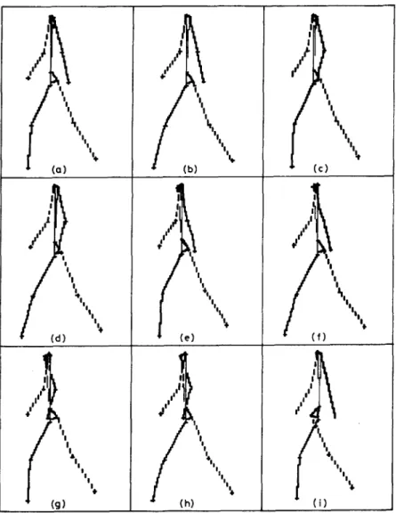
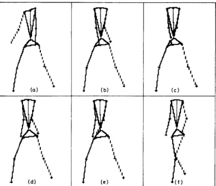
To show the further pruning power of our algorithm, the above recovered body configurations of frame 1 in both sequences will be analyzed to a greater degree. First we shall use the grouping routine to combine those macroscopically similar body configurations for frame 1 of both sequences. As a consequence, the thirty-two body configurations of SEQl are reduced to 16, as shown in Fig. 6; the six body configurations of SEQ2 remain the same, as shown in Fig. 8.

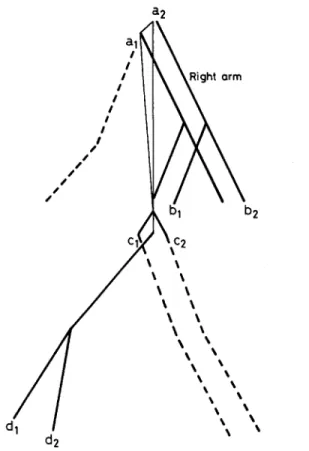
Now we shall apply Rules 3-5 of the walking-model constraints to refine the results given above. For the convenience of analysis, we superimpose the sixteen body configurations of SEQl to give a new figure, i.e., Fig. 7. In this figure there are two solutions for the right shoulder, labeled as “a,” and “a,.” Since the right elbow

I’

I+

,i

I

i

I I 'I iI ‘I 'I 't (c)

i

I’

3“

I’

)

'I I I $1, 'I '5 t (f) : I' I' ,I: i'l "5 'I 'I 'I 'I '5 (i)

FIG. 6. Recovered body configurations for frame 1 of SEQl. These views are obtained by a perspective projection of a human body onto the zcy, plane. The left arm and left leg are in dashed lines; the right arm and right leg are in wiggled solid lines.

3D HUMAN BODY POSTURES 163 I’ ,I; t’ I’ i I I ‘I 'I 'I t (PI FIG. 6-Continued.

swings backward, so we can reject the solution “ui,” which was shown to correspond to a forward swing, according to Rule 3. Similarly, we reject the solution of the left hip labeled by “ci.” By Rule 5, we require that the right leg be stretched, so we reject the rear solution of the left ankle labeled by “d2.” At this moment we have only two body configurations left. The nonuniqueness is due to two possible solutions of the right wrist labeled by “bi” and “bz”; both are legal. If preferred, one may use some extra rule to argue that the body contiguration with the stretched right arm, i.e., the one labeled by “b2,” is the better solution. This solution is precisely the given input data.

Next, consider the six body contigurations of SEQ2. We can hnd the body configuration of Fig. 8(c) is the final unique solution as follows. The body configura- tion of Fig. S(a) has a twisted torso, as indicated by the fact that the left shoulder is closer to the camera, while the left hip is farther from the camera. The body

FIG. 7. Superposition of the recovered body configurations for frame 1 of SEQl.

configurations of Figs. 8(b) and 8(d) have the left arm located on a plane which is not parallel to the moving direction; the moving direction is dictated by the normal vector of the head plane. So, by Rule 4, we can eliminate these body configurations. Similarly, the right arm of the body configuration of Fig. 8(e) and the left leg of the body configuration of Fig. 8(f) violate Rule 4, too. Therefore, only the body configuration of Fig. 8(c) satisfies all rules. This is exactly the given input data.

5. SUMMARY

We have provided a method to determine the 3D body configuration from a single view. That is, by using the coordinates of the six feature points on the head and their perspective projections, a transformation matrix [T] is found. From the transforma- tion matrix, we can establish the relationships of the 14 body joints in the camera coordinate system. Under the assumption of fixed lengths of body segments, we can derive the 3D coordinates of all joints sequentially, starting from the neck. However, there are many possible combinations of joint coordinates because of the joint positional ambiguity. We propose to use a binary interpretation tree as a representa- tion scheme for all possible body configurations and develop a tree-pruning process to reduce the number of possible interpretations.

The beauty of the tree pruning is made possible by the use of physical constraints and motion constraints. We formally introduce a common coordinate system in

3D HUMAN BODY POSTURES 165 f I I I i I I I (e) + -I-

FIG. 8. Recovered body configurations for frame 1 of SEQ2. These views are obtained by a

perspective projection of a human body onto the tcyC plane.

which we derive all necessary formulas needed for applying the two types of constraints.

We use two sets of input data generated by a walking-simulation program, called SEQl and SEQ2. First we show the various phenomena of tree pruning under the effect of physical constraints. Second, we indicate the remarkable pruning power of the first two general rules of walking-model constraints.

In pursuit of a possible unique solution, we introduce the concept of cooperative movement and more stringent rules of the walking model. By using these rules and the grouping procedure, we are able to obtain two final solutions for frame 1 in SEQl and a unique solution for frame 1 in SEQ2.

Currently we are investigating methods for deriving a unique solution of the body configuration for each individual frame based on a dynamic analysis of a sequence of frames [22]. To show the effectiveness of this approach we allow more solutions of body configurations associated with each frame. So we do not apply stringent rules in the tree pruning process. The early results show the approach is very promising.

APPENDIX: INPUT DATA

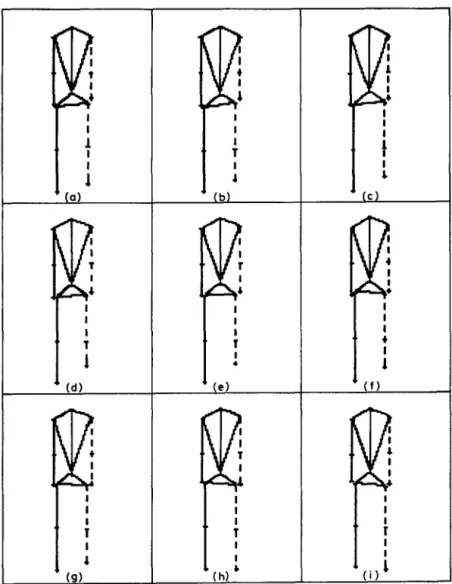
Figure A.1 shows a portion of the first input image sequence SEQl. The second input image sequence SEQ2 can be found in the dissertation [22]. These data are generated by a walking-simulation program, as described in [lo, 191. The camera which takes these pictures is located at (400,0,0) in SEQl and (300,0,300) in SEQ2 in the head-centered coordinate system, aiming at the walking person. The coordi- nate system is defined such that the x axis is in the moving direction, the y axis is

vertical to the ground surface, and the z axis is horizontal to the ground surface. The sampling rate is 0.2 s per frame.

Table A.1 lists the lengths of rigid segments of the walking person mentioned above. Table A.2 shows the 3D coordinates of the feature points on the head in the head-centered coordinate system and the corresponding 2D perspective projections on the image plane for frame 1 of SEQl. Notice that the last four feature points on the head are coplanar. However, this property does no harm in finding the solution to Eq. (3), i.e., [A]*W = 0.

I I +

I I

p’

I

f I

1

(9)

I

I r 1 b

$

I I ; I . (e)

I

r+

I

T

I

I J I I / (h) ’

f

/ Ci)’

FIG. A.l. Input image sequence, SEQl. The person is walking toward the camera. The camera is located at (400,0,0) in the head-centered coordinate system. These views are shown in the y, z coordinate system.

3D HUMAN BODY POSTURES 167

TABLE A.1

Lengths of Rigid Segments of a Human Body Rigid segment name Length (cm)

Neck-to-shoulder 20.5 Neck-to-pelvis 46.3 Shoulder-to-pelvis 50.2 Shoulder-to-elbow 30 Elbow-to-wrist 26 Pelvis-to-hip 19 Hip-to-knee 38 Knee-to-ankle 31 Shoulder-to-shoulder 40.3 Hip-to-hip 32.2 TABLE A.2 Input Head Data

(a) 3D Coordinates of the feature points in the head-centered coordinate system

X _Y z Neck - 34.168 52.103 0.000 Nose - 29.168 61.603 0.000 Right eye - 32.168 65.103 5.500 Left eye - 31.168 65.103 - 5.500 Right ear - 35.168 60.103 8.500 Left ear - 35.168 60.103 - 8.500

(b) 2D Perspective projections of head feature points in frame 1 of SEQl in the camera-centered coordinate system

X’ _{Y ’} Neck Nose Right eye Left eye Right ear Left ear - 0.00024 0.59320 - 0.00025 0.70944 - 0.06329 0.74631 0.06280 0.74631 - 0.09680 0.68273 0.09631 0.68273

REFERENCES

1. D. Marr and T. Poggio, A computational theory of human stereo vision, Proc. R. Sot. London Ser. B 204,1979, 301-328.

2. B. K. P. Horn, Obtaining shape from shading information, in The Psychoiogv of Computer Vision (P. H. Winston, Ed.), McGraw-Hill, New York, 1975.

3. B. K. P. Horn, Understanding image intensities, Artif. Intell. 8, 1977, 201-231.

4. A. P. Witkin, Recovering surface shape and orientation from texture, Art& Intell. 17,1981.

5. J. R. Kender, Shape from Texture, Ph.D. dissertation, Carnegie-Mellon University, Nov. 1980. 6. D. Marr, Analysis of occluding contour, Proc. R. Sot. Landon Ser. B 197,1977, 441-475.

7. S. Ullman, The interpretation of structure from motion, Proc. R. Sot. London Ser. B 2@3, 1979,

405-426. _

8. J. W. Roach and J. K. Aggarwal, Determining the movement of objects from a sequence of images, IEEE Trans. Pattern Anal. Mach. Intell. PAMI-2, Dec. 1980, 554-562.

9. A. Z. Meiri, Chr monocular perception of 3-D moving objects, IEEE Trans. Pattern Anal. Mach. Intell. PAMI-2, Nov. 1980, 582-583.

10. R. F. Rashid, LIGHT: A System for Interpretation of Moving Light Displays, Ph.D. dissertation, Computer Science Dept., Univ. Rochester, Rochester, N.Y., April 1980.

11. L. G. Roberts, Machine perception of three-dimensional solids, in Optical and Electra-Optical Information Processing (James T. Tippett et al., Ed.) pp. 159-197, MIT Press, Cambridge, 1965. 12. D. F. Rogers and J. A. Adams, Mathematical Elements for Computer Graphics, McGraw-Hill, New

York, 1978.

13. S. T. Barnard and W. B. Thompson, Disparity analysis of images, IEEE Trans. Pattern Anal. Mach. Intell. PAMI-2, July 1980,333-340.

14. R. F. Rashid, Toward a system for the interpretation of moving light displays, IEEE trans. Pattern Anal. Mach. Intell. PAMI-2, Nov. 1980, 574-581.

15. J. O’Rourke, Image Analysis of Human Motion, Ph.D. dissertation, The Moore School of Electrical Engineering, Univ. of Pennsylvania, 1980.

16. J. O’Rourke and N. I. Badler, Model-based image analysis of human motion using constraints propagation, IEEE Trans. Pattern Anal. Mach. Intell. PAMI-2, Nov. 1980.

17. J. A. Webb and J. K. Aggarwal, Structure from motion of rigid and jointed objects, Artif. Intell. 19, 1982, 107-130.

18. N. I. Badler and S. W. SmoIiar, Digital representations of human movement, Comput. Surveys 11,

March 1979,19-38.

19. J. E. Cutting, A program to generate synthetic walkers as dynamic point-light displays, Behav. Res. Methods Instrum. 10 (I), 1978, 91-94.

20. G. Johansson, Spatial-temporal differentiation and integration in visual motion perception, Psych. Res. 38, 1976, 379-391.

21. J. Panero and M. Z&r&, Human Dimension and Interior Space, Watson-Guptill, New York, 1979. 22. H. J. Lee, Computer Vision for 30 Human Motion Analysis, Ph.D. dissertation, Institute of Computer

Engrg., National Chiao Tung Univ., Hsinchu, Taiwan, R.O.C., July 1984.

23. M. Herman, Understanding Body Postures of Human Stick Figures, Ph.D. dissertation, Univ. of Maryland, 1979.