Motion of a Colloidal Sphere Covered by a Layer of Adsorbed
Polymers Normal to a Plane Surface
Jimmy Kuo and Huan J. Keh1
Department of Chemical Engineering, National Taiwan University, Taipei 106-17 Taiwan, Republic of China
Received June 29, 1998; accepted November 9, 1998
A combined analytical–numerical study is presented for the slow motion of a spherical particle coated with a layer of adsorbed polymers perpendicular to an infinite plane, which can be either a solid wall or a free surface. The Reynolds number is assumed to be vanishingly small, and the thickness of the surface polymer layer is assumed to be much smaller than the particle radius and the spacing between the particle and the plane boundary. A method of matched asymptotic expansions in a small parameterl incorpo-rated with a boundary collocation technique is used to solve the creeping flow equations inside and outside the adsorbed polymer layer, wherel is the ratio of the characteristic thickness of the polymer layer to the particle radius. The results for the hydrody-namic force exerted on the particle in a resistance problem and for the particle velocity in a mobility problem are expressed in terms of the effective hydrodynamic thickness (L) of the polymer layer, which is accurate to O(l2). The O(l) term for L normalized by its
value in the absence of the plane boundary is found to be inde-pendent of the polymer segment distribution and the volume fraction of the segments. The O(l2) term for L, however, is a
sensitive function of the polymer segment distribution and the volume fraction of the segments. In general, the boundary effects on the motion of a polymer-coated particle can be quite significant. © 1999 Academic Press
Key Words: particle motion; adsorbed polymers; hydrodynamic thickness; boundary effect.
1. INTRODUCTION
Adsorption of polymers from solution onto various solid surfaces has been a subject of both theoretical (1–7) and experimental (8 –15) interest. A colloidal dispersion can be stabilized in either an aqueous or a nonaqueous continuous phase by solvated polymers adsorbed on the particle surfaces (16, 17). The polymeric chains attached to the surface can be regarded as a barrier around each particle, preventing their close approach to one another. Another spectacular effect of such adsorption is the restriction of flow in capillary pores due to the effective decrease in size (18, 19). This effect influences many technologically important processes such as
ultrafiltra-tion, gel permeation chromatography, and enhanced oil recov-ery.
A polymer chain adsorbs on an interface through contacts distributed randomly along the chain. These contacts result from attractive forces between polymer segments and the in-terface, generally attributed to van der Waals forces, hydrogen bonding, or Coulombic (charge– charge, dipole– dipole, etc.) interactions. The structure of an adsorbed polymer layer de-pends on the nature of the polymer, the solvent, and the interface. In general, adsorbed polymer chains have only part of their segments on the interface while a substantial fraction of the segments are protruding into the solution. Sequences of segments attached to the interface are “trains,” nonadsorbed sequences with adsorbed segments at both ends are “loops,” and sequences that leave the interface and never return are “tails” (1, 6, 20).
Since an adsorbed polymer layer is diffuse, there is no unique measure of its thickness. One convenient definition, applicable to both colloidal particles and micropores, is the hydrodynamic thickness which is the distance the “no-slip” boundary condition on the fluid velocity must be moved into the fluid phase to produce the same hydrodynamic effect as the polymer layer. For the case of a polymer layer that is thin relative to the radii of curvature of the solid surface, previous theoretical analyses (21–23) predict the same value of the hydrodynamic thickness for different external flows and geom-etries, given the same local rheological model for flow within the surface layer. Among the methods used to determine the hydrodynamic thickness of an adsorbed polymer layer are sedimentation, viscometry, microelectrophoresis, and photon correlation spectroscopy (14, 24).
The steady-state motion of a single spherical particle cov-ered by a layer of adsorbed polymers was analyzed by Ander-son and Kim (23) using a method of matched asymptotic expansions (singular perturbations) to solve the generalized Brinkman equation for the flow field inside the polymer layer and the Stokes equations for the flow field outside the layer. The result for the drag force produced by the fluid on the translating particle, expressed as the hydrodynamic thickness of the adsorbed polymer layer, is accurate to O(l2), wherel is the ratio of the polymer-layer length scale to the particle radius. 1To whom correspondence should be addressed.
296
0021-9797/99 $30.00
Copyright © 1999 by Academic Press All rights of reproduction in any form reserved.
Their calculations indicated that (i) the O(l2) term is negative, meaning the hydrodynamic thickness decreases as the particle radius decreases assuming all other conditions are constant, (ii) the free-draining assumption for flow through the polymer chains applies accurately for calculating the hydrodynamic thickness if the Stokes radius of the polymer segments is much smaller than the length scale of the polymer layer, and (iii) the presence of only a small amount of adsorbed polymer tails can make a significant contribution to the hydrodynamic thickness if the length scale of the tails exceeds the length scale of the loops by a factor of two or more. On the other hand, the creeping flow of an incompressible Newtonian fluid past a composite sphere having a central solid core and an outer uniform porous shell was solved by Masliyah et al. (25) using the Stokes and Brinkman equations. An analytical formula for the drag force experienced by the particle was derived as a function of the radius of the solid core, the thickness of the porous shell, and the permeability of the shell.
In most technical applications, colloidal particles with or without adsorbed polymer layers are not isolated and the sur-rounding fluid is externally bounded by solid or fluid surfaces (e.g., container walls and interfaces between two fluid phases). Thus, it is important to determine if the presence of neighbor-ing boundaries significantly affects the movement (such as sedimentation and diffusion) of the particles. Recently, Ander-son and Solomentsev (26) examined motions of a spherical particle covered by a layer of adsorbed polymers near an infinite plane wall and along the centerline of a long cylindrical tube. Using the concept of hydrodynamic thickness and a method of reflections together with the technique of matched asymptotic expansions, they determined the boundary effects on the particle movement to O(l2) in increasing powers ofj up to O(j3), where j is the ratio of the particle radius to the
distance between the particle center and the boundary. On the other hand, the quasisteady motion of a polymer-coated sphere located at the center of a spherical cavity has been investigated (27). A combined analytical–numerical exact solution of the hydrodynamic effects exerted by the cavity wall on the moving particle accurate to O(l2) was also obtained using the method
of matched asymptotic expansions.
The purpose of this paper is to obtain an exact solution to the quasisteady problem of the motion of a polymer-coated sphere perpendicular to a nearby plane surface to O(l2). The plane surface can be either a solid wall or a free surface. The momentum equation applicable to the system is solved by using the method of matched asymptotic expansions incorpo-rated with a boundary collocation technique (28, 29). Our numerical results for the motion of a particle normal to a plane wall compare favorably with the formulas analytically derived from the method of reflections. It is found that the effect of the plane surface on the movement of the polymer-coated particle can be significant when the surface-to-surface spacing becomes small.
2. ANALYSIS
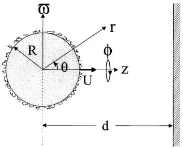
Consider the quasisteady motion of a spherical particle of radius R covered by a layer of adsorbed polymers in a New-tonian liquid in the direction normal to an infinite planar surface located at a distance d from the particle center, as shown in Fig. 1. Here, (v#, f, z) and (r, u, f) denote circular cylindrical and spherical coordinates, respectively, and the origin of coordinates is chosen at the particle center. The thickness of the adsorbed polymer layer surrounding the par-ticle is characterized by a length scaled (based on loops if both loops and tails are present). In general, the length scale of a surface polymer layer depends on the molecular weight of the polymer, the amount of the polymer adsorbed, and the relative interactions among the polymer, interface, and fluid. It is assumed thatd is small in comparison with R and d 2 R. So, the thin polymer layer is not in contact with the planar surface. The particle velocity equals Uez, where ez is a unit vector in
the z (axial) direction. The Reynolds number is assumed to be much smaller than unity.
The fluid velocity and dynamic pressure fields, v and p, are governed by the modified Stokes equations (23)
¹ z $m@¹v 1 ~¹v!T#% 2 ¹p 2zrf @v 2 v~ p!# 5 0, [1a]
¹ z v 5 0. [1b]
In Eq. [1a],z is the friction coefficient of an isolated polymer segment,r is the density of polymer segments at the position in question, v( p)is the velocity of the segments, f is a function of r accounting for hydrodynamic interactions among seg-ments, andm is the local fluid viscosity which is also a function ofr. The density distribution of the segments in the loops and tails cannot yet be determined experimentally. Previous theo-retical studies (1, 6, 30) established that the density of polymer
FIG. 1. Geometrical sketch of the motion of a polymer-coated sphere perpendicular to a plane surface.
segments in the loops decays exponentially with the distance from the surface of adsorption and the segment density in the tails can exceed the value in the bulk solution much farther from the surface. The effective viscositym in the polymer layer is not a measurable quantity. Previous calculations for an isolated sphere (23) have shown that the effects of the differ-ence betweenm and the constant bulk solvent viscosity msand of the hydrodynamic interactions among polymer segments are negligible. Therefore, we assume m 5 ms and f 5 1 (free draining) throughout the surface polymer layer in this work. It is understood that v( p)equals the particle velocity Uez in the
surface layer surrounding the translating particle.
Owing to the axisymmetric nature of the flow, it is conve-nient to introduce the Stokes stream functionC which satisfies Eq. [1b] and is related to the velocity components in spherical coordinates by vr5 2 1 r2 sinu C u , vu5 1 r sinu C r . [2a,b]
Taking the curl of Eq. [1a] and applying Eqs. [1b] and [2] gives a fourth-order linear partial differential equation forC,
E4C 2l22
S
bE2C 1db drC
r
D
5 0, [3]where the dimensionless parametersb and l are defined as
b 5d 2zr ms , l 5
d
R, [4a,b]
and the axisymmetric Stokesian operator E2is given by
E25 2 r21 sinu r2 u
S
1 sinu uD
. [5]In Eqs. [3] and [5], dimensionless variables are used, with r normalized by the particle radius R and C by UR2. The hydrodynamic parameter b denotes the ratio of the frictional force exerted by the polymer segments on the fluid to the viscous force of the bulk fluid and is O(1) with respect tol which has been assumed to be small.
Because the fluid velocity satisfies the no-slip requirement at the fluid–solid interfaces of the particle and the wall and the fluid is motionless far away from the particle, the boundary conditions for the case of the motion of a polymer-coated sphere perpendicular to a solid plane are:
r5 R: v 5 Uez, [6a]
z5 d: v 5 0, [6b]
r3` and z , d: v 5 0. [6c]
For the case that the polymer-coated sphere is moving normal to a planar free surface, boundary condition [6b] is replaced by
z5 d: vz5 0 and vv#
z 50, [7a,b]
where vz and vv# are the velocity components in cylindrical
coordinates. The deformation of the free surface produced by the approaching particle will not be considered here.
The drag force exerted on the particle surface r5 R by the fluid (in the z direction) is (31)
F5pms
E
0 p r3 sin3u rS
E2C r2 sin2uD
rdu. [8]In terms of the equivalent hydrodynamic thickness L of the adsorbed polymer layer, the drag force is given by the Stokes law with a wall correction,
F5 26pms~R 1 L!UK. [9]
For the system specified by Eq. [6], the wall correction factor K for a “bare” sphere of radius R equals22D20/3RU, where D20 is defined later by Eq. [17]. The hydrodynamic thickness L can be expressed as
L5 ARl~1 1 Bl! 1 O~l3!.
[10] By combining Eqs. [8]–[10] after solving Eqs. [3] and [6] for
C, one can obtain dimensionless parameters A and B. Note
that K $ 1, A is positive, and B represents the correction for the particle curvature. Also, A and B (or L) depend on the segment density distribution of the surface polymer layer and the parameter R/d, but are independent of the particle velocity. Equation [3] poses a singular perturbation problem whenl
! 1. In the “outer region,” where r 2 R @ Rl, one has b 5
0 and the solution for the stream function can be written as (28, 29)
C~O!5 C
W1 CS. [11]
HereCW is a solution of the Stokes equation (E4C 5 0) in cylindrical coordinates that represents the disturbance pro-duced by the planar surface and is given by a Fourier–Bessel integral, CW5
E
0 ` v#J1~tv#!@X~t! 1 zY~t!#etz dt, [12]and X(t) and Y(t) are unknown functions of t.CSis a solution of the Stokes equation in spherical coordinates representing the disturbance generated by the polymer-coated sphere and is given by CS5
O
n52 ` ~Cnr2n111 Dnr2n13!Gn21/ 2~n!, [13] Cn5 Cn01 Cn1l 1 Cn2l21 . . . , [14a] Dn5 Dn01 Dn1l 1 Dn2l21 . . . , [14b]where Gn21/ 2(n) is the Gegenbauer polynomial of the first kind
of order n and degree 21/2, n is used to denote cos u for brevity, and Cnm and Dnm are unknown constants. The
Ge-genbauer polynomials are related to the Legendre polynomials via the relation
Gn21/ 2~n! 5
1
2n2 1 @Pn22~n! 2 Pn~n!#. [15] A solution of the form given by Eqs. [11]–[13] immediately satisfies boundary condition [6c].
Substitution of the solution C(O) given by Eqs. [11]–[13] into the boundary condition [6b] or [7] and application of the Hankel transform on the variablev# leads to a solution for X(t) and Y(t) in terms of the unknown constants Cnand Dn. After
the substitution of this solution into Eq. [12], the resulting stream function for the outer region is given by (29)
C~O!5
O
n52 `O
m50 ` lm@Cnmbn~v#, z! 1 Dnmdn~v#, z!#, [16]where the functionsbn(v#, z) and dn(v#, z) are defined by Eqs. [A1] and [A2] (for the case of a solid plane) or Eqs. [A3] and [A4] (for the case of a planar free surface) in Appendix A. The unknown constants Cnm and Dnm in Eq. [16] are to be
deter-mined by matching C(O) with the solution to Eq. [3] in the “inner region.” The solution of Cn0and Dn0(and also the wall
correction factor K) has been obtained numerically by Keh and Tseng (29) who studied the motion of a “bare” sphere normal to an infinite plane using the boundary collocation method.
Substituting Eq. [16] into Eq. [8] and utilizing the orthogo-nality properties of the Gegenbauer polynomials results in the simple relation
F5 4pmsD25 4pms~D201 D21l 1 D22l21 . . .!. @17#
The combination of Eqs. [9], [10], and [17] yields
A5D21 D20
, B5D22 D21
. [18a,b]
Within the “inner region” near the particle, where r2 R ' O(Rl), a solution for the stream function is sought in the form
C~I!5 U
O
n52 ` @l2 Fn2~ y! 1l3 Fn3~ y! 1 . . .#Gn21/ 2~n!, [19]where y5l21(r2 R). Note that this expression is used when the reference frame travels with the particle. Substituting Eq. [19] into Eqs. [3] and [6a] and collecting terms of equal orders inl produces the following equations for functions Fnm( y) up to m 5 3, R d 3 Fn2 d y3 2 b R dFn2 d y 5 0, [20a] y5 0: Fn25dFn2 d y 5 0; [20b] R d 3 Fn3 d y3 2 b R dFn3 d y 5 cn, [21a] y5 0: Fn35 dFn3 d y 5 0, [21b]
where n5 2, 3, 4, . . . , and cnare integration constants to be determined by matching the inner and outer solutions.
The unknown boundary conditions on Fnmat y3` and the
constants Cnm and Dnm can be determined by matching Eqs.
[16] and [19] at equivalent orders inl, lim y3`C ~I!5 lim y3`@C ~O!11 2Ur 2~1 2n2!#r 5R1ly. [22]
The second term in the brackets accounts for the difference in the reference frames used forC(O)andC(I). After performing this matching we obtain the equations
05 W0~n! 112R2~1 2n2!, [23a] 05 W1~n! 1 yX0~n! 1 Ry~1 2 n2!, [23b] lim y3`n
O
52 ` Fn2Gn21/ 2~n! 5 W2~n! 1 yX1~n! 1 y2 Y0~n! 112y2~1 2n2!, [23c] lim y3`nO
52 ` Fn3Gn21/ 2~n! 5 W3~n! 1 yX2~n! 1 y 2 Y1~n! 1 y3 Z0~n!, [23d] where the functions Wk(n), Xk(n), Yk(n), and Zk(n) with k 50, 1, 2, and 3 are defined by Eqs. [A7]–[A10] (for the case of a solid wall) or Eqs. [A11]–[A14] (for the case of a free surface) in Appendix A.
With the solution of the constants Cn0 and Dn0 obtained
numerically by using the boundary collocation technique (29), Eq. [23a] and the derivative of Eq. [23b] with respect to y are immediately satisfied. The constants Cn1 and Dn1 are to be
determined by solving Eq. [23b] and the derivative of Eq. [23c] with the knowledge of Cn0and Dn0, and then the constants Cn2
and Dn2 are to be determined by solving Eq. [23c] and the
derivative of Eq. [23d]. The useful result is obtained in the following form: D215 RUg
O
n52 ` snbn, [24a] D225 U lim y3`nO
52 `F
pnS
dFn3 d y 2 cn 2 Ry 22 dn yD
1 qnS
Fn2 R 1 bn 2 Ry 22 b ngyDG
. [24b]On the other hand, taking the differentiation of Eqs. [23c,d] with respect to y twice and solving them by utilizing the orthogonality properties of the Gegenbauer polynomials, we obtain
lim y3` d2 Fn2 d y2 5 2bn, [25a] lim y3` d2 Fn3 d y2 5 cn y R1 dn. [25b]
In Eqs. [24] and [25], g is defined later by Eq. [32a], and the constants sn, pn, qn, bn, cn, and dn, which depend on the separation
parameter R/d only, can be numerically determined using the boundary collocation technique. Knowing thatb 5 0 as y 3 `, one can find that Eqs. [20a] and [21a] are consistent with Eq. [25].
If we define new functions G( y) and H( y) as
G5 1 b2 dF22 d y , H5 1 c2 dF23 d y , [26a,b] then Eqs. [20], [21], and [25] give
Rd 2 G d y22 b RG5 0, [27a] y5 0: G 5 0, [27b] y3`: dG d y 321; [27c] Rd 2 H d y22 b RH5 1, [28a] y5 0: H 5 0, [28b] y3`: dH d y3 y R1 d2 c2 . [28c]
Due to its linearity Eq. [28] can be decomposed into two parts, with one part given by
R d 2 H9 d y2 2 b RH9 5 1, [29a] y5 0: H9 5 0, [29b] y3`: dH9 d y 3 y R, [29c]
and the other in the form of Eq. [27], where
H5 H9 2d2 c2
G. [30]
If functions Fn2and Fn3, instead of F22and F23, are selected
to define the functions G and H in Eq. [26], the same equations as Eqs. [27]–[30] will be resulted.
The parameters A and B in Eq. [10] are obtained from Eqs. [18], [24], [26], and [30] as A5 1 D20 RUg
O
n52 ` snbn, [31a] B5 1 D20A RU@VO
n52 ` ~ pncn1 qnbn! 2gO
n52 ` pndn#, [31b] where g 5 lim y3` 1 R ~G 1 y!, [32a] V 5R12E
0 ` ~G 1 y 2 Rg!d y. [32b]In Eq. [31], the numerical solution of D20is known (29) and the
constants sn, pn, qn, bn, cn, and dncan be determined using the
boundary collocation technique. Note that parameters A and B can be expressed in terms of the function G( y) only. After obtaining the solution of G in Eq. [27] for a given polymer segment density distribution r( y) (b is related to r by Eq. [4a]), parameters A and B can be evaluated from Eqs. [31] and [32].
Whenb 3 0 (or z 3 0), the surface layer of the polymer-coated particle does not exert any resistance to the fluid motion. For this limiting case, the solution of Eq. [27] is G5 2y and Eqs. [33] and [32] yieldg 5 V 5 0 and A 5 B 5 0; viz., the particle behaves like a “bare” sphere of radius R as expected.
When the particle and the planar surface are separated by an infinite distance (i.e., R/d 3 0), the interaction between the particle and the planar boundary vanishes. For this limiting case, K 5 1, D205 23RU/ 2, s25 p25 q25 1, b25 c2
5 23/ 2, d25 3g`/ 2, and all the constants sn, pn, qn, bn, cn,
and dnfor n $ 3 are zero. Thus, Eq. [31] reduces to
A`5g`5 lim y3` 1 R ~G`1 y!, [33a] B`5g`1 2 R2g `
E
0 ` ~G`1 y 2 Rg`!d y. [33b]Here, the subscript “`” is used to represent the limiting case of R/d 3 0. Both theoretical calculations (23) and experimental data (9, 12) showed that the value of B`would be negative, meaning the hydrodynamic thickness of the adsorbed polymer layer increases with the particle radius assuming all other conditions are constant. If the surface layer is a dense film of thickness d, in which no flow is permitted relative to the particle, one has A` 5 1 and B` 5 0.
The drag force exerted on the particle surface written by Eq. [9] can also be expressed as
F5
S
11L` RD
@1 1 gl 1 hl 21 O~l3!#KF~0! , [34] where L`5 A`Rl~1 1 B`l! 1 O~l3! [35] and F(0) 5 26pmsRU, which is the drag force on a “bare”sphere moving with velocity U in the absence of the plane surface. Here, the hydrodynamic thickness of the adsorbed polymer layer is taken to be a constant equal to the value when the boundary is not present (L`), and the wall correction is given by an expansion inl in the brackets of Eq. [34].
For a mobility problem, in which the velocity of the particle is to be determined for a specified force acting on the particle, the particle velocity can be written as
U5
S
11L RD
21 K21U~0! 5 @1 2 Al 1 ~ A22 AB!l21 O~l3!#K21U~0! 5S
11L` RD
21 @1 1 gl 1 hl21 O~l3!#21K21U~0!. [36]Here, U(0)5 2F/(6pmsR), which is the velocity of a “bare” sphere subject to an applied force2F in the absence of the plane surface.
A comparison between Eqs. [9] and [34] yields
g5 A 2 A`, [37a]
h5 AB 2 A`B`2 A`~ A 2 A`!. [37b]
By the linearity of the problem, the same values of A and B (or g and h) are predicted for a given combination of the segment density distribution of the surface polymer layer and the pa-rameter R/d whether the particle is approaching the plane surface or receding from it. In the following section, numerical calculations show that A . A`(or g . 0) for all cases with a finite value of R/d.
TABLE 1
Numerical Results of A/A` and B/B`for a Polymer-Coated Sphere Moving Perpendicular to a Plane Surface with Various Values of Parameters R/d andb0for Systems with No Polymer Tails
R/d A/A`
B/B`
K
b05 10 b05 100 b05 1000
Motion normal to a solid plane
0 1 1 1 1 1 0.1 1.1252 0.5490 20.2510 21.4512 1.1262 0.2 1.2780 0.0153 21.7312 24.3515 1.2851 0.3 1.4662 20.6305 23.5223 27.8610 1.4884 0.4 1.7069 21.4615 25.8273 212.377 1.7563 0.5 2.0337 22.6138 29.0231 218.639 2.1255 0.6 2.5154 24.3537 213.849 228.095 2.6695 0.7 3.3136 27.2941 222.005 244.075 3.5594 0.8 4.9169 213.262 238.556 276.506 5.3053 0.9 9.7886 231.361 288.757 2174.87 10.441 0.95 19.6 — — — 20.576
Motion normal to a planar free surface
0 1 1 1 1 1 0.1 1.0808 0.7072 0.1880 20.5911 1.0810 0.2 1.1746 0.3683 20.7520 22.4329 1.1756 0.3 1.2863 20.0441 21.8960 24.6745 1.2878 0.4 1.4264 20.5908 23.4121 27.6450 1.4242 0.5 1.6160 21.3913 25.6325 211.996 1.5967 0.6 1.9002 22.6968 29.2535 219.091 1.8283 0.7 2.3916 25.1133 215.956 232.223 2.1708 0.8 3.4557 210.495 230.884 261.473 2.7724 0.9 7.1185 228.102 279.716 2157.15 4.3331 0.95 15.486 264.378 2180.33 2354.30 7.1416 b05 10: A`5 3.4570, B`5 20.9509 b05 100: A`5 5.7596, B`5 20.5712 b05 1000: A`5 8.0622, B`5 20.4081
3. RESULTS AND DISCUSSION
The numerical results for the motion of a colloidal sphere covered by a layer of adsorbed polymers perpendicular to an infinite planar surface are presented in this section. The hydrodynamic parame-ters A and B are calculated from Eqs. [31] and [32] in which the function G( y) can be obtained by numerically solving Eq. [27], and the constants sn, pn, qn, bn, cn, and dnare numerically
deter-mined using the boundary collocation technique. The only poly-mer-layer property that is required in solving the function G( y) is
b, which is related to the segment density r(y) by Eq. [4a].
Following Anderson and Kim (23), we assume that the segment density has a form of two exponentially decaying distributions,
r~ y! 5 r0~e2y/d1he2ay/d!, [38]
where the primary distribution (r0e2y/d) represents segments in the loops and the secondary distribution denotes the tails.a is the ratio of loop-to-tail length scales for the polymer layer and is smaller than unity. It can be found from Eq. [38] that the fraction of segments contained in the tails ish/(h 1 a). Theories based on lattice statistics (1, 4, 6, 30) have shown that the segment density in tails increases with the distance from the interface, then passes through a maximum, followed by an exponential decrease with a decay length which is about twice (or more in some cases) that of the segment density in loops. At very small distances from the interface the loops prevail over the tails, while the outer part of the adsorbed layer is completely dominated by the tails. The function form expressed by Eq. [38] is a simple and reasonable approxi-mation for the segment density distribution as long ash and a are small (say,h/(h 1 a) # 0.3 and a # 0.5). Substituting Eq. [38] into Eq. [4a] yields the dimensionless hydrodynamic function
b~ y! 5 b0~e2y/d1he2ay/d!, [39]
where the surface density parameter b0 5 d2zr0/ms, which
has typical values in the range 10 –1000 (23).
The parameters A and B for a polymer-coated sphere moving normal to a solid plane wall or a planar free surface normalized by their values in the absence of the plane boundary ( A` and B`) can be evaluated for a given distri-bution ofb(y) as expressed by Eq. [39]. In our calculations, the Runge–Kutta–Fehlbery method (32) was employed to obtain the numerical solutions of the function G( y). Results of A/A`and B/B`for various values of separation parameter R/d are given in Table 1 for systems with no tails (h 5 0). Three constant values 10, 100, and 1000 are chosen for the surface hydrodynamic parameter b0 and the values of A` and B`for each case are also listed in this table. Note that, although A`(or g) is an increasing function ofb0, the ratio A/A` (or g/A`) is independent of this parameter. For the motion of a sphere normal to a solid plane wall or a planar free surface, the boundary effects increase the value of A (or the equivalent hydrodynamic thickness L of the adsorbed polymer layer, or the resistance coefficient2F/6pmsRUK of the polymer-coated sphere) and the ratio A/A` (or g/A`) increases monotonically and rapidly with the increase of parameter R/d. In the limit R/d3 0, there is no boundary interaction effect and A5 A`(or g5 0). On the other hand, the ratio B/B`decreases monotonically from unity and soon becomes negative (or the value of B increases monotonically from B`, which is negative, and soon becomes positive) when R/d increases from zero. It means that, when the polymer-coated sphere is situated near a plane boundary with a given value of R/d, the equivalent hydrodynamic thickness L of the adsorbed polymer layer decreases with the increase of the particle radius R assuming all other condi-tions are constant. For a fixed value of R/d, the value of B/B` decreases with the increase of b0. In general, when the
TABLE 2 Numerical Results of A/A`and (A22 AB)/(A
` 2 2 A
`B`) for a Polymer-Coated Sphere Moving Perpendicular to a Solid Plane Wall
with Various Values of Parameters R/d and b0 for Systems with No Polymer Tails as Obtained from the Boundary Collocation Technique (Listed in Column KK) and the Method of Reflections (Ref. 26, Listed in Column AS)
R/d (A22 AB)/(A`2 2 A`B `) A/A` b05 10 b05 1000 b05 1000 KK AS KK AS KK AS KK AS 0.1 1.1252 1.1250 1.1262 1.1267 1.1263 1.1267 1.1264 1.1267 0.2 1.2780 1.2731 1.2852 1.2884 1.2863 1.2886 1.2867 1.2887 0.3 1.4662 1.4367 1.4866 1.4960 1.4898 1.4975 1.4909 1.4980 0.4 1.7069 1.5950 1.7468 1.7556 1.7532 1.7615 1.7553 1.7635 0.5 2.0337 1.7057 2.0970 2.0487 2.1071 2.0665 2.1103 2.0725 0.6 2.5154 1.7013 2.5998 2.2859 2.6133 2.3267 2.6175 2.3403 0.7 3.3136 1.5201 3.3972 2.2588 3.4104 2.3275 3.4144 2.3506 0.8 4.9169 1.1963 4.8934 1.7521 4.8900 1.8343 4.8871 1.8619 0.9 9.7886 0.9374 8.9228 0.9845 8.7830 1.0644 8.7288 1.0911
parametersb0and R/d are kept constant, a solid plane wall produces a larger value of A/A`and a smaller value of B/B` (or stronger boundary effect) than a planar free surface does. For convenience in using Eqs. [9], [34], and [36] to evaluate the drag force or translating velocity of the particle moving normal to a plane surface, we also list the values of K as a function of R/d in Table 1. It can be found that the difference in values of A/A` and K is quite small when R/d is small.
Note that the boundary effect on the particle velocity can be very significant when R/d approaches unity.
To seek the solution to the problem expressed by Eqs. [11] and [16] as series in powers ofl, we have assumed that the series in Eq. [10] converges. On the other hand, the numerical calculations presented in Table 1 indicate a slow convergence of Eq. [10] (viz. A @ 1 and B @ 1) as R/d approaches unity and b0 is large. Under this particular situation, the perturbation solution presented here is useful only when the value ofl is extremely small. Indeed, addi-tional analysis which is not limited to the assumptionl ! 1 is needed to check on the validity of the expansion in l introduced by Eq. [10].
In an earlier paper (33), the present authors studied the hydrodynamic interactions between two spherical particles covered by adsorbed polymer layers translating along the line of their centers in an unbounded fluid using a similar boundary collocation method. If one considers two identical polymer-coated spheres of radius R separated by a center-to-center distance 2d approaching or moving away from each other with equal velocities and divides the fluid domain in half along the plane of symmetry between the spheres, this plane then becomes the free surface in the case analyzed in this work. The results of A/A`and B/B`obtained here for a planar free surface agree very well with the previous results for all values of R/d. (Due to a sign error in the computer program for numerical calculations, the results of B/B` in this earlier paper are not as accurate as those presented in Table 1.)
Using a method of reflections, Anderson and Solomentsev (26) analytically solved the mobility problem of a polymer-coated sphere moving near a solid plane wall. For the axisym-metric motion considered here, their result gives
A5 A`K
H
12S
R dD
3 1 OFS
RdD
4GJ
, [40a] A22 AB 5 KH
A`22 A `B`2 1 4~ A` 22 A `B`1 6V`! 3S
RdD
3 1 OFS
RdD
4GJ
, [40b] where the definitions of K andV`have been given in Eqs. [9] and [32b], respectively. In Table 2, the values of A/A`and ( A22 AB)/( A`2 2 A`B`) calculated from the above asymptotic
solution with the O[(R/d)4] terms neglected are compared with our collocation results. As expected, the asymptotic for-mula [40] from the method of reflections agrees well with our exact results only when the separation parameter R/d is small. Note that formula [40] always underestimates the ratio A/A` and overestimates the ratio B/B`when R/d is small.
We next consider the effect of tails in the adsorbed polymer layer surrounding the particle. Equation [27] is solved for G( y)
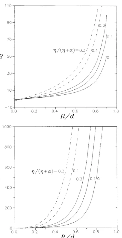
FIG. 2. The parameters B and h for the motion of a polymer-coated sphere perpendicular to a solid plane wall as a function of R/d withb05 100. The
solid curves are plotted for the case ofa 5 0.5 and the dashed curves are plotted for the case ofa 5 0.25.
over a range ofh and a. The results of parameters B and h for the motion of a polymer-coated sphere normal to a solid plane wall as functions of the separation parameter R/d are plotted in Fig. 2 for typical cases of the fraction of polymer segments contained in the tails,h/(h 1 a). The curve of parameter A (or g) is not drawn since the ratio A/A`is not a function ofh/(h
1a) or a and its results were presented in Table 1. It can be
seen that the increase of the segment fraction in the tails or the
increase of the relative length of the tails (with a decrease ina) will increase the boundary effect on B and h when all the other conditions are unchanged. This influence can be quite signifi-cant when the value of a is less than 0.5. It implies that the interaction between the polymer-coated particle and the bound-ary is to a large extent determined by long dangling tails.
4. CONCLUDING REMARKS
The slow motion of a spherical particle coated with a layer of adsorbed polymers moving perpendicular to an infinite plane, which can be either a solid wall or a free surface, has been analyzed in this work. The analysis provides governing equations and boundary conditions which can be solved using the boundary collocation technique, given the polymer segment density distri-bution r(y) or hydrodynamic function b(y), to determine the parameters A and B of Eq. [10] or parameters g and h of Eq. [34]. The hydrodynamic force exerted on the particle can be calculated using Eq. [9] and the results of A and B; that is correct to O(l2). For the exponential polymer segment distribution given by Eq. [38], the ratio A/A`(or g/A`) is found to be independent of the values ofb0,a, and h/(h 1 a), and its results for various values of R/d are listed in Table 1. The dependence of B and h onb0,a,
h/(h 1 a), and R/d is given in Table 1 and Fig. 2. The results
indicate that the boundary effects on the motion of a polymer-coated particle can be significant when the separation distance is small. For example, the equivalent hydrodynamic thickness of the adsorbed polymer layer for a particle located near a solid wall with R/d5 0.5 (or 0.8) is about twice (or five times) of that for the particle far away from the wall. These effects cannot be ignored when one observes the sedimentation or other motions of poly-mer-coated particles near a boundary.
Throughout the calculations in the previous section we have assumed a simple exponential decay of the polymer segment density. This could be an oversimplification since the convex nature of the particle surface might adjust the excluded volume effects among the polymer segments. A segment density of the following form was suggested (23) to allow for curvature effects on polymer distribution:
r~ y! 5 r011 s~ y/R!e2y/d i5 1, 2, [41]
where s should be a positive value. For systems with no tails,
b( y) has the form of the above equation with r0replaced by
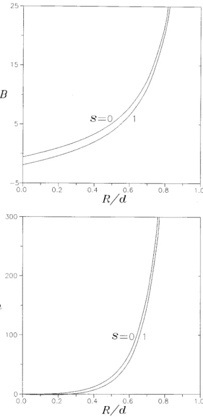
b0. It is understood that parameters A` and A (or g) are independent of the curvature coefficient s. We have numeri-cally solved the same problem considered in the previous section but with the segment distribution given by Eq. [41] to compute parameters B and h. These calculations, which are plotted in Fig. 3 for the case of a solid plane wall, indicate that the values of B and h decrease with the increase of s for various values of R/d as one would expect.
FIG. 3. The parameters B and h for the motion of a polymer-coated sphere perpendicular to a solid plane wall as a function of R/d with the segment density distribution given by Eq. [41] andb05 100.
One may wish to consider a polymer segment distribution that has the same adsorbed amount as for the exponential distribution but is uniform over a distance from the particle surface:
r~ y! 5 r0 if 0# y #d, [42a]
r~ y! 5 0 if y $ d. [42b]
For this profile,b( y) has the form of Eq. [42] with r0replaced byb0and it can be shown that
A`5 1 2b021/ 2tanhb01/ 2, [43a] B`5 2 1 A`b0~1 2 sechb0 1/ 2!2 . [43b]
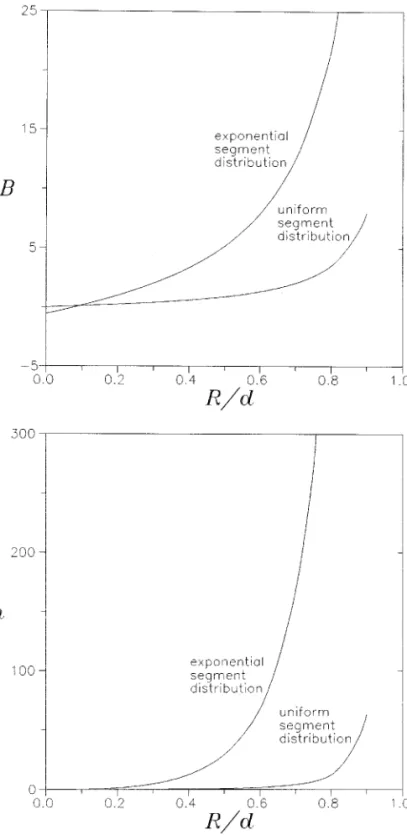
It can be found that the value of A`is about six times greater (if b0 ' 100) for an exponential distribution of segments than for the polymer uniformly distributed over a region of thicknessd. Although A`is a function ofb0for this segment distribution, the ratio A/A`(or g/A`) is independent of the segment distribution and its results have been given in Table 1. In Fig. 4, the numerical results of parameters B and h for the motion of a polymer-coated sphere normal to a solid plane wall versus R/d obtained using Eq. [42] for the seg-ment distribution are plotted. The corresponding results for the case of an exponential distribution of segments are also plotted in the same figure for comparison. It can be seen that the boundary effect on B and h is much stronger for the exponential distribution of segments over a distance from the particle surface than for the uniform distribution of segments.
In addition to obtaining suitable approximate solutions of the quasisteady equations of motion of a polymer-coated sphere normal to a plane surface, it is desirable to know how well the predicted effects will be realized physically. The experimental work has lagged behind the theory in this area. However, if the segment density distribution in the surface polymer layer r(y) together with the dimensionless surface density parameterb0is determined independently, one can measure the velocity and drag force experienced by a poly-mer-coated sphere moving normal to a plane surface in a viscous fluid for various values of the separation parameter and choose the values of l to test the theoretical analysis developed in this work.
APPENDIX A
For conciseness the definitions of some functions in Section 2 are listed here. The functionsbn(v#, z) and dn(v#, z) in Eq. [16] are defined by (29) bn~v#, z! 5 bˆn~v#, z! 2 bˆn~v#, 2d 2 z! 2 2~n 1 1!~d 2 z!bˆn11~v#, 2d 2 z!, [A1] dn~v#, z! 5 dˆn~v#, z! 2 dˆn~v#, 2d 2 z! 1 2~n 2 2!~d 2 z!bˆn21~v#, 2d 2 z! 2 2~2n 2 3!d~d 2 z!bˆn~v#, 2d 2 z!, [A2]
FIG. 4. The parameters B and h for the motion of a polymer-coated sphere perpendicular to a solid plane wall as a function of R/d with the segment density distribution given by Eq. [42] andb05 100. The corresponding results
for the case of the motion of a sphere normal to a solid plane, and
bn~v#, z! 5 bˆn~v#, z! 2 bˆn~v#, 2d 2 z!, [A3]
dn~v#, z! 5 dˆn~v#, z! 22nn2 3~2d 2 z!bˆn21~v#, 2d 2 z!
1n2 3n bˆn22~v#, 2d 2 z!, [A4]
for the case of the motion of a sphere normal to a planar free surface. In the above equations,
bˆn~v#, z! 5~v#21 z12!~n21!/ 2Gn21/ 2
F
z ~v#21 z2!1/ 2G
, [A5] dˆn~v#, z! 5~v#21 z12!~n23!/ 2Gn21/ 2F
z ~v#21 z2!1/ 2G
. [A6]The functions Wk(n), Xk(n), Yk(n), and Zk(n) in Eq. [23]
are defined by Wk~n! 5
O
n52 ` $Cnk@22~n 1 1!a0,n,12g0,n21,01 R2n11Gn21/ 2~n!# 1 Dnk@22~2n 2 3!da0,n21,11 2~n 2 2!a0,n22,1 2g0,n23,21 R2n13Gn21/ 2~n!#%, [A7] Xk~n! 5O
n52 ` $Cnk@22~n 1 1!a1,n,12g1,n21,0 2 ~n 2 1! R2nG n 21/ 2~n!# 1 Dnk@22~2n 2 3!da1,n 21,1 1 2~n 2 2!a1,n22,12g1,n23,2 2 ~n 2 3! R2n12G n 21/ 2~n!#%, [A8] Yk~n! 5O
n52 ` $Cnk@22~n 1 1!a2,n,12g2,n21,0 11 2n~n 1 1! R 2n21G n 21/ 2~n!# 1 Dnk@22~2n 2 3!da2,n21,11 2~n 2 2!a2,n22,1 2g2,n23,2112~n 2 2!~n 2 3! R2n11Gn21/ 2~n!#% , [A9] Zk~n! 5O
n52 ` $Cnk@22~n 1 1!a3,n,12g3,n21,0 21 6~n 2 1!n~n 1 1! R 2n22G n 21/ 2~n!# 1 Dnk@22~2n 2 3!da3,n21,11 2~n 2 2!a3,n22,1 2g3,n23,2216~n 2 1!~n 2 2!~n 2 3! R 2nG n 21/ 2~n!#% , [A10] for the case of a solid plane, andWk~n! 5
O
n52 `H
Cnk@2g0,n21,01 R2n11Gn21/ 2~n!# 1 DnkF
n2 3n g0,n23,02 2n2 3 n a0,n22,1 1 R2n13G n 21/ 2~n!GJ
, [A11] Xk~n! 5O
n52 `H
Cnk@2g1,n21,02 ~n 2 1! R2nGn21/ 2~n!# 1 DnkF
n2 3 n g1,n23,02 2n2 3 n a1,n22,1 2 ~n 2 3! R2n12G n 21/ 2~n!GJ
, [A12] Yk~n! 5O
n52 `H
CnkF
2g2,n21,01 1 2n~n 1 1! R 2n21G n 21/ 2~n!G
1 DnkF
n2 3n g2,n23,02 2n2 3 n a2,n22,1 1 12~n 2 2!~n 2 3! R2n11G n 21/ 2~n!GJ
, [A13] Zk~n! 5O
n52 `H
CnkF
2g3,n21,02 1 6~n 2 1!n~n 1 1! 3 R2n22G n 21/ 2~n!G
1 D nkF
n2 3 n g3,n23,0 22nn2 3 a3,n22,12 1 6~n 2 1!~n 2 2! 3 ~n 2 3! R2nG n 21/ 2~n!GJ
, [A14]for the case of a planar free surface. Here,am,n,kandgm,n,kare functions ofn defined by a0,n,k5 ~kd 2 Rn!gn,0,k, [A15] a1,n,k5 ~kd 2 Rn!~gn,1,k1 hn,0,k! 2ngn,0,k, [A16] a2,n,k5 ~kd 2 Rn!~gn,2,k1 hn,1,k1 mn,0,k! 2n~gn,1,k1 hn,0,k!, [A17] a3,n,k5 ~kd 2 Rn!~ gn,3,k1 hn,2,k1 mn,1,k1 nn,0,k! 2n~gn,2,k1 hn,1,k1 mn,0,k!, [A18] g0,n,k5 gn21,0,k, [A19] g1,n,k5 gn21,1,k1 hn21,0,k, [A20] g2,n,k5 gn21,2,k1 hn21,1,k1 mn21,0,k, [A21] g3,n,k5 gn21,3,k1 hn21,2,k1 mn21,1,k1 nn21,0,k. [A22] In Eqs. [A15]–[A22], gn,m,k5 x12n/ 2Gn111k,m, [A23] hn,m,k5 2nx12~n12!/ 2y1Gn111k,m, [A24] mn,m,k5 n 2@~n 1 2! x12~n14!/ 2y1 2 2 x12~n12!/ 2#Gn111k,m, [A25] nn,m,k5 n~n 1 2! 6 @2~n 1 4! x1 2~n16!/ 2y 1 3 1 3x12~n14!/ 2y 1#Gn111k,m, [A26] where Gn,05 Gn21/ 2~t!, [A27] Gn,15 1 ~2n 2 1!
H
1 2n23O
k50 ^n22& ~21!k~n 2 k 2 2!! k!~n 2 2k 2 3!!~n 2 k 2 2!! 3 tn22k22u2 1 2n21O
k50 ^n& ~21!k~n 2 k!! k!~n 2 2k 2 1!!~n 2 k!!t n22kuJ
, [A28] Gn,25 1 2~2n 2 1!H
1 2n23O
k50 ^n22& ~21!k~n 2 k 2 2!! k!~n 2 2k 2 3!!~n 2 k 2 2!! 3 tn22k22@~n 2 2k 2 3!u21 2v# 221n21O
k50 ^n& ~21!k~n 2 k!! k!~n 2 2k 2 1!!~n 2 k!! 3 tn22k@~n 2 2k 2 1!u21 2v#J
, [A29] Gn,35 1 6~2n 2 1!H
1 2n23O
k50 ^n22& ~21!k~n 2 k 2 2!! k!~n 2 2k 2 3!!~n 2 k 2 2!! 3 tn22k22@~n 2 2k 2 3!~n 2 2k 2 4!u3 1 6~n 2 2k 2 3!uv 1 6w# 221n21O
k50 ^n& ~21!k~n 2 k!! k!~n 2 2k 2 1!!~n 2 k!! 3 tn22k@~n 2 2k 2 1!~n 2 2k 2 2!u3 1 6~n 2 2k 2 1!uv 1 6w#J
. [A30]In Eqs. [A27]–[A30],^n& 5 0 if n 5 0, ^n& 5 (n 2 1)/ 2 if n is odd,^n& 5 (n 2 2)/ 2 if n is even, and
t5 2x121/ 2z1, [A31] u5nz1212 x121y1, [A32] v512~3x122y1 2 2 x121!, [A33] w512nz121~3x122y1 22 x121! 21 2~5x1 23y 1 32 3x122 y1!. [A34]
In Eqs. [A23]–[A26] and [A31]–[A34],
x15 R21 4d22 4Rnd, [A35]
y15 R 2 2nd, [A36]
z15 Rn 2 2d. [A37]
APPENDIX B Nomenclature
A, B parameters defined by Eq. [10]. A`, B` parameters defined by Eq. [33]. bn, cn, dn coefficients defined by Eq. [24].
Cn, Dn coefficients defined by Eq. [13], m n12/s,
mn/s.
Cnm, Dnm coefficients defined by Eq. [14], m n12/s,
mn/s.
d distance between the center of particle and the planar surface, m.
ez unit vector in the z direction.
f parameter for the hydrodynamic interactions among polymer segments defined by Eq. [1a].
F hydrodynamic force exerted on the particle, N. Fnm functions of y defined by Eq. [19], m
2
. g, h parameters defined by Eq. [34].
G, H, H9 functions of y defined by Eqs. [26]–[30], m. Gn21/ 2 Gegenbauer polynomial of order n and
de-gree21/2.
K wall correction factor defined by Eq. [9]. L effective hydrodynamic thickness of the
polymer layer defined by Eq. [10], m. L` effective hydrodynamic thickness of the
polymer layer defined by Eq. [35], m. p hydrodynamic pressure, N/m2.
Pn Legendre polynomial of order n. pn, qn, sn coefficients defined by Eq. [24]. r radial spherical coordinate, m. R particle radius, m.
s curvature coefficient defined by Eq. [41]. U translational velocity of the particle, m/s.
v fluid velocity, m/s.
v( p) velocity of polymer segments, m/s.
Wk, Xk, Yk, Zk functions ofn defined by Eqs. [A7]–[A14],
m3/s, m2/s, m/s, s21.
y l21(r 2 R), m.
z axial coordinate, m.
a ratio of loop-to-tail length scales for a poly-mer layer.
b function of y defined by Eq. [4a].
b0 parameter defined by Eq. [39].
bn, dn functions ofv# and z defined by Eqs. [A1]– [A4].
g parameter defined by Eq. [32a].
d length scale of the polymer layer surrounding the particle, m.
z Stokes friction coefficient of a polymer seg-ment, kg/s.
h fraction of tails as defined by Eq. [38].
u, f angular spherical coordinates.
l d/R.
m viscosity inside a polymer layer, kg/m s.
ms fluid viscosity, kg/m s.
n cosu
r polymer segment distribution, m23.
r0 polymer segment density in loops at the sur-face, m23.
C Stokes stream function, m3/s.
C(O)
stream function in the outer region, m3/s.
C(I)
stream function in the inner region, m3/s.
CS, CW stream functions defined by Eq. [11], m 3
/s.
v# radial cylindrical coordinate, m.
V parameter defined by Eq. [32b].
ACKNOWLEDGMENT
Part of this work was supported by the National Science Council of the Republic of China.
REFERENCES
1. Roe, R. J., J. Chem. Phys. 44, 4264 (1966). 2. Silberberg, A., J. Chem. Phys. 48, 2835 (1968). 3. deGennes, P. G., Rep. Prog. Phys. 32, 187 (1969). 4. Hesselink, F. Th., J. Colloid Interface Sci. 50, 606 (1975).
5. Dimarzio, E. A., and Rubin, R. J., J. Polym. Sci. Polym. Phys. Ed. 16, 457 (1978). 6. Scheutjens, J. M. H. M., and Fleer, G. J., J. Phys. Chem. 84, 178 (1980). 7. Anderson, J. L., McKenzie, P. F., and Webber, R. M., Langmuir 7, 162
(1991).
8. Doroszkowski, A., and Lambourne, R., J. Colloid Interface Sci. 26, 214 (1968).
9. Garvey, M. J., Tadros, Th. F., and Vincent, B., J. Colloid Interface Sci. 55, 440 (1976).
10. Kato, T., Nakamura, K., Kawaguchi, M., and Takahashi, A., Polym. J. 13, 1037 (1981).
11. Cohen Stuart, M. A., Waajen, F. H. W. H., Cosgrove, T., Vincent, B., and Crowley, T. L., Macromolecules 17, 1825 (1984).
12. Baker, J. A., Pearson, R. A., and Berg, J. C., Langmuir 5, 339 (1989). 13. Kim, J. T., and Anderson, J. L., Ind. Eng. Chem. Res. 30, 1008 (1991). 14. Siffert, B., and Li, J. F., Colloids Surfaces 62, 307 (1992).
15. Carvalho, B. L., Tong, P., Huang, J. S., Witten, T. A., and Fetters, L. J.,
Macromolecules 26, 4632 (1993).
16. Napper, D. H., “Polymeric Stabilization of Colloidal Dispersions.” Aca-demic Press, London, 1983.
17. Hunter, R. J., “Foundations of Colloid Science,” Vol. I. Clarendon Press, Oxford, 1986.
18. Gramain, Ph., and Myard, Ph., Macromolecules 14, 180 (1981). 19. McKenzie, P. F., Kapur, V., and Anderson, J. L., Colloids Surf. A 86, 263
(1994).
20. Ploehn, H. J., and Russel, W. B., Adv. Chem. Eng. 15, 137 (1990). 21. Varoqui, R., and Dejardin, P., J. Chem. Phys. 66, 4395 (1977). 22. Hatano, A., Polymer 25, 1198 (1984).
23. Anderson, J. L., and Kim, J., J. Chem. Phys. 86, 5163 (1987). 24. Kawaguchi, M., and Takahashi, A., Adv. Colloid Interface Sci. 37, 219
(1992).
25. Masliyah, J. H., Neale, G., Malysa, K., and van de Ven, T. G. M., Chem.
Eng. Sci. 42, 254 (1987).
26. Anderson, J. L., and Solomentsev, Y., Chem. Eng. Comm. 148 –150, 291 (1996).
27. Keh, H. J., and Kuo, J., J. Colloid Interface Sci. 185, 411 (1997). 28. Dagan, Z., Pfeffer, R., and Weinbaum, S., J. Fluid Mech. 122, 273 (1982). 29. Keh, H. J., and Tseng, C. H., Int. J. Multiphase Flow 20, 185 (1994). 30. Fleer, G. J., Cohen Stuart, M. A., Scheutjens, J. M. H. M., Cosgrove, T., and
Vincent, B., “Polymers at Interfaces.” Chapman & Hall, London, 1993. 31. Happel, J., and Brenner, H., “Low Reynolds Number Hydrodynamics.”
Martinus Nijhoff, The Netherlands, 1983.
32. Gerald, C. F., and Wheatley, P. O., “Applied Numerical Analysis,” 5th ed. Addison-Wesley, Reading, MA, 1994.