A novel congestion control mechanism for multicast real-time connections
Jau-Hsiung Huang, Chun-Chuan Yang*, Nai-Cheng Fang
Communications and Multimedia Laboratory Department of Computer Science and Information Engineering National Taiwan University, Taipei, Taiwan R.O.C.
Received 8 August 1997; received in revised form 24 September 1998; accepted 24 September 1998
Abstract
Time framing strategies such as Stop-and-Go (S&G) [Golestani S.J., Congestion-free transmission of real-time traffic of real-time traffic in packet networks, IEEE INFOCOM, 1990, pp.527-536; Golestani S.J., A framing strategy for congestion management, IEEE JSAC, 9(7), 1991, pp.1064-1077; Golestani S.J., Congestion-free communication in high-speed packet networks, IEEE Trans. on Communications, 39(12), 1991, pp.1802-1812; Golestani S.J., A stop-and-go queueing framework for congestion management, ACM SIGCOMM, 1992, pp.8-18] and Continuous Framing (CF) [Jau-Hsiung Huang, Biau-Jwo Tsaur, Continuous framing mechanism for congestion control in broadband networks, Computer Communications, 18(10), 1995, pp.718-724] are designed to support the end-to-end delay bound and jitter bound for unicast connections. Considering the features of real-time multicast connections, a new time framing mechanism named Multicast Contin-uous Framing (MCF) is proposed in this article. S&G and CF allow only one time frame length per connection, but MCF allows changing of the time frame length of a connection at intermediate nodes so that the statistical multiplexing gain within a connection is increased, i.e., the bandwidth requirement can be reduced. We also present the multicast connection setup scheme for MCF in the article. Simulation results show that MCF has a much better performance than that of CF, and the tighter jitter bound a connection requests, the more performance improvement MCF can obtain.䉷 1999 Elsevier Science B.V. All rights reserved.
Keywords: Real-time; Stop- and -Go; MCF
1. Introduction
The problem of congestion control has been the subject of extensive research for computer networks. Traditionally, acknowledgment-based control, such as window-based flow control, makes use of the information fed by the down-stream or the destination node to regulate the input traffic. In broadband networks, the propagation delay, when measured in terms of the service time of a packet, is much longer than that in narrowband networks; consequently, the acknowl-edgement-based control mechanism is not suitable.
In addition, the window-based flow control and first-come-first-serve policy can neither satisfy some perfor-mance requirements, such as bounded end-to-end delay and loss free transmissions, nor provide firewalls among connections. Thus, some rate-based congestion control mechanisms [1–5] have been proposed. These control mechanisms include Fair Queueing (FQ) [6], Hierarchical
Round Robin (HRR) [7], Real-Time Virtual Clock (Real-Time VC) [8, 9], Delay–Earliest-Due-Date (Delay–EDD)
[10], and Jitter–Earliest-Due-Date (Jitter–EDD) [11], Rate
Controlled Static Prioriy (RCSP) [12], Stop-and-Go (S and
G) [13–16], Continuous Framing (CF) [17], and
General-ized Processor Sharing [19, 20].
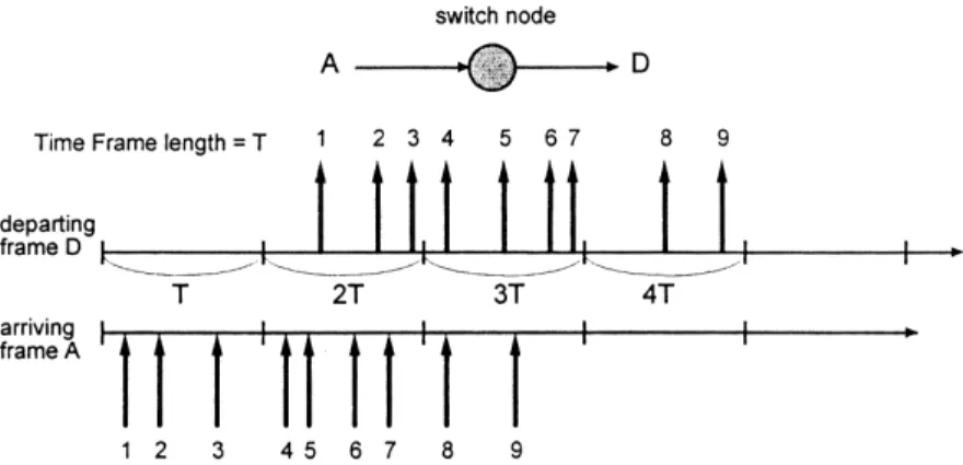
Among these control mechanisms, S&G [13–16] guaran-tees a bounded end-to-end delay and loss free transmission for real-time applications. Bandwidth reservation for each connection is determined by the admission control based on peak rate requirement. S&G adopts a time framing strategy to separate time into frames. Under the framing architecture, S&G requires that packets arriving in the kth frame should be sent out in the (k⫹ 1)th frame as shown in Fig. 1, in which the time frame length is assumed to be T. In this way, packets will not suffer more than T queuing time at each intermediate node and therefore a bounded delay can be provided along the path. In S&G, it is desirable to incorpo-rate multiple frame sizes according to different delay requirements. However, the frame size of longer ones must be integer multiples of that of the smaller ones.
As the arriving frame and the departing frame of a switch node are not always synchronized as in Fig. 1, S&G intro-duces an extra delay, which is called the synchronization
delay, for each packet to smooth the skew between arriving
frame and the departing frame. Hence, the synchronization delay incurs a larger end-to-end delay.
0140-3664/99/$ - see front matter䉷 1999 Elsevier Science B.V. All rights reserved. PII: S 0 1 4 0 - 3 6 6 4 ( 9 8 ) 0 0 2 6 0 - 6
* Corresponding author. Tel.: ⫹ 886 49 910960 ext. 4131; fax: ⫹ 886 4 2116689; e-mail: [email protected]
The CF [17] scheme was proposed to eliminate the synchronization delay incurred in S&Gsuch that the end-to-end delay bound is reduced from 2HT to HT, where H is the hop count of the connection. In order to remove the synchronization delay, the time framing structures of the incoming and the outgoing links should be perfectly synchronized. That is, for a connection j which passes through an intermediate node i with incoming link Lin and
outgoing link Lout, node i should start a time frame on Loutfor
connection j as soon as a time frame finishes on Lin. To
achieve this, CF requires the source node to send packets uniformly within a frame as shown in Fig. 2, and adds an end flag in the last packet within a frame to identify the end of the time frame, as packets 3 and 7 in the figure. Thus, as long as the switch node sees a packet with the end flag, it knows that the incoming frame has been finished and a new frame should be started immediately on the outgoing link. The packets are then transmitted uniformly over the new frame.
With this mechanism, the time frames of different connections on a link do not need to begin or end at the same time. As the framing structures on Lin and Lout are
perfectly synchronized, there will be no synchronization delay at each node. Under such a mechanism, a packet will suffer only a delay of T on each intermediate node,
Hence the end-to-end delay can be bounded by HT. Other than that if the end-to-end delay bound is reduced by half, CF can improve the link utilization by 40% for many cases as shown in [17].
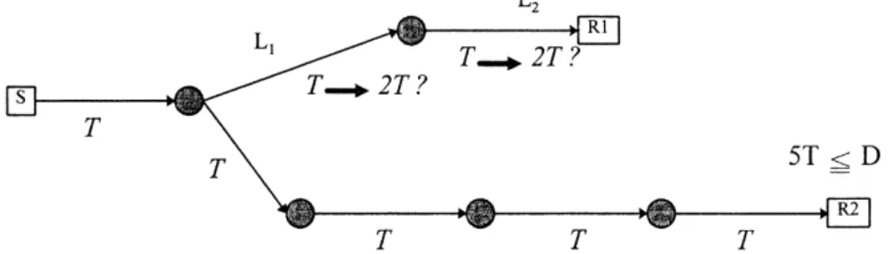
Both S&G and CF were designed for unicast connections. When applying them to multicast connections, we found that the network resources could be easily wasted. A typical example of the routing tree for a multicast connection is shown in Fig. 3. It is reasonable to assume that the end-to-end delay requirements for all destinations of the multicast connection are the same. We denote the delay requirement as D. Using CF, the time frame length T of the connection is determined by the path from the source to the farthest desti-nation, as the path S-R2 in Fig. 3. Hence, T should not be larger than D/5 in this case where 5 is the link count between S and R2. However, the bounded delay on the path from S to R1 will equal D*3/5, which is smaller than what is required. If we enlarge the frame lengths of links L1and L2to 2T, the
delay requirement from S to R1 is still met while the effi-ciency of links L1 and L2 can also be improved. This is
because the larger the time frame, the more statistical multi-plexing gain we can get from a connection; i.e. less band-width is required for the connection.
CF provides only one time frame length for a connection along the path, and it does not allow the switch node to change the frame length once the length is decided. There-fore, CF needs to be modified to improve the efficiency of network utilization for multicast connections as explained above. A modification of CF, named as Multicast
Contin-uous Framing (MCF) scheme, is proposed in the article to
allow the length of the time frame to be changed in switch nodes.
The article is organized as described next. The concept of MCF is given in section 2, and the admission control, end-to-end delay, and jitters of MCF are also presented in the section. The connection setup scheme for multicast connec-tions is presented in section 3. In section 4, we present several simulation results of MCF for performance evalua-tion. Lastly, section 5 concludes this article.
J.-H. Huang et al. / Computer Communications 22 (1999) 56–72 57
Fig. 1. The concept of Stop-and-Go.
2. Multicast continuous framing 2.1. General concept of MCF
MCF adopts the same framing concept as CF does, i.e. sending packets uniformly in a time frame and using end flags to indicate the ends of time frames. The objective of MCF is to allow changes of the time frame length along the path of a connection. In MCF, each connection selects its own set of time frame lengths. The frame length of longer ones in the set is assumed to be integer multiples of that of the smaller ones. That is, if a connection selects G time frame lengths, T1⬎ T2⬎ … ⬎ TG, they satisfy the
follow-ing relationship: Ti Ki*Ti⫹1; Ki僆 N; i 1 ⬃ G ⫺ 1.
The basic idea of MCF is to record the information of all time frame lengths in the header of each packet. More speci-fically, MCF identifies each kind of time frame used in a connection by the end flag of each time frame in the packet header. For example, a packet with the end flags of time frames Tiand Tjimplies the packet is the end packet of both Tiand Tj. The operations in MCF are divided into two parts: at the source node and at the intermediate nodes. The source node performs the actions of recording all time frame infor-mation in the packets, and the intermediate nodes perform the actions of changing the time frame if required according to the information recorded in the packets. Next we present the control actions of the source and the intermediate nodes.
2.1.1. MCF control at the source node
As there is only one frame length allowed along the path of a connection in CF, packets only need a one-bit field to indicate if the packet carries an end flag. MCF allows a set of time frames used for a connection, so the packet in MCF must have one end bit for each kind of time frame. The flow control field of a MCF packet is shown in Fig. 4. There are G end flag bits followed by a group number in the flow control field in which G is the number of frame sizes used in the connection. The group number is used in changing the time frame at the intermediate nodes, and the physical interpreta-tion of the group number is explained next.
We assume time frames T1, T2,…, TG are used for a
connection and Ti Ki*Ti⫹1 as mentioned in section 2.1. Tmax and Tminare assumed to be the maximum time frame
and the minimum time frame respectively; i.e., Tmax T1 and Tmin TG. Toutdenotes the selected output time frame
of the source node.
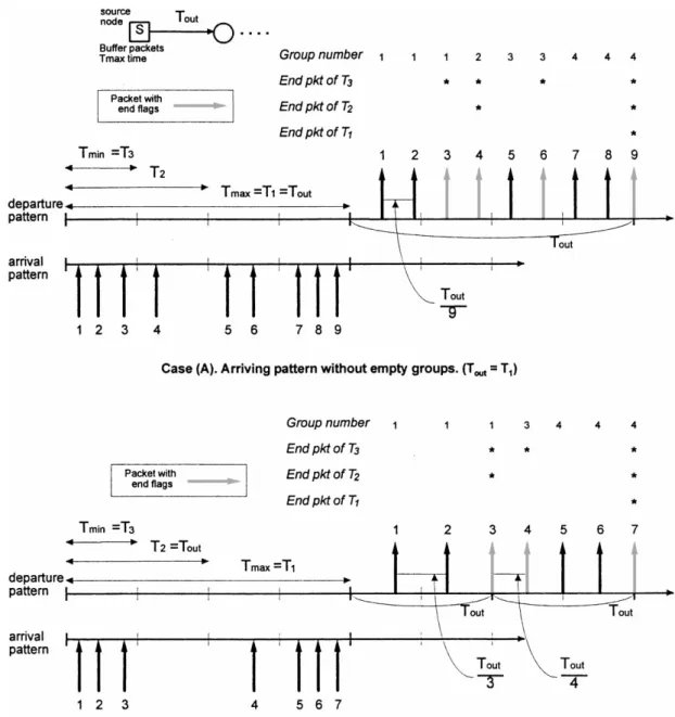
In order to set the end flags of all time frames for input packets, the arriving packets must be buffered Tmaxtime at
the source node. The source node adds end flags in the end packets of different time frames T1, T2,…,TG, and records
the values of the group number in each packet, in which we define the last packet arrived in a time frame as the end packet of that frame. The group number of a packet in the buffered Tmaxtime is the sequence number of the Tminframe
which the packet is in. For example, suppose Tmax 4Tmin which means there are 4Tminframes within the buffered Tmax
time at the source node, the group number of a packet arrived in the first Tmin frame has a value of 1 and the
group number of a packet arrived in the second Tminframe
has a value of 2, and the group number of a packet arrived in the last Tminframe has a value of 4. The assignment process
of the group number is repeated every Tmaxtime.
The source node then sends out packets uniformly within the selected output time frame Tout. As Toutis one of the G
time frames, the packets which were buffered Tmax time
could be sent out in several Tout frames. For example, if
Tmax 4Tmin and Tout 2Tmin, i.e. 2 Tout Tmax, packets are buffered Tmaxtime and sent out in two Toutframes. The
packets with group number 1 or 2 are sent out uniformly within the first Tout frame, and the packets with group
number 3 or 4 are sent out uniformly within the second
Toutframe.
Examples for the operations at the source node are given in Fig. 5 in which three kinds of different time frames T1, T2,
and T3are chosen for the connection in which T1 2T2and T2 2T3. Fig. 5 shows operations for two different arrival patterns and two different Toutselections, Tout T1for case (A) and Tout T2 for case (B). From the arrival pattern of case (A), packets 3, 4, 6, and 9 are end packets of T3, packets
4 and 9 are end packets of T2, and packet 9 is the end packet
Fig. 3. An example of multicast routing tree.
of T1. An asterisk (*) is added above the end packets of the
corresponding time frame. As packets 1, 2, and 3 arrived in the first Tminframe, the group number of these packets is 1,
packet 4 arrived in the second Tmin frame, so its group
number is 2, etc. As Toutin case (A) equals Tmax, all packets
buffered are sent out uniformly within the next Tout frame,
i.e., the nine buffered packets are spaced by Tout/9 in case
(A) of Fig. 5.
For the arrival pattern of case (B), there is no packet arriving in the second Tminframe, and thus no packet has a
group number of 2. As Tout T2 and 2 Tout Tmax, the buffered packets are sent out in two consecutive Toutframes.
Packets with group number 1 or 2 (i.e. packets 1, 2, and 3) are sent out uniformly within the first Toutframe, and packets
4, 5, 6, and 7 whose group number is either 3 or 4 are sent out uniformly within the second Toutframe.
2.1.2. MCF control at the intermediate nodes
The end flags and group number carried by packets are used in changing the time frame length at the intermediate node. In this section, we only present the mechanism to change the time frame length instead of the selection of the time frame length. The strategy of selecting the time frame length is presented in section 3. One of following three situations may occur when an intermediate node serves a connection: (1) the length of the arrival time frame and that of the departure time frame are equal, (2) the length of the arrival time frame is a multiple of the J.-H. Huang et al. / Computer Communications 22 (1999) 56–72 59
length of the departure time frame, and (3) the length of the departure time frame is a multiple of the length of the arrival time frame. Operations of the intermediate nodes for tion (1) are the same as those in CF. Operations for situa-tions (2) and (3) that require changing the time frame are described in the next section.
2.1.2.1. Changing a time frame into smaller ones. Suppose that the arrival time frame is Taand the departure time frame
is Td. We assume Ta K*Td, Td J*Tmin, J; K 僆 N. The intermediate node buffers the incoming packets until an end packet of Ta arrives. Next, the intermediate node starts K
consecutive Tdframes. The node sends packets with group
number [1⬃ J] uniformly within the first Td frame, and
sends packet with group number [J⫹ 1 ⬃ 2J] uniformly within the second Td frame, etc. In this way, the traffic
pattern from the Td’s point of view can be reconstructed in
the departure frames of the intermediate node. An example is illustrated in Fig. 6.
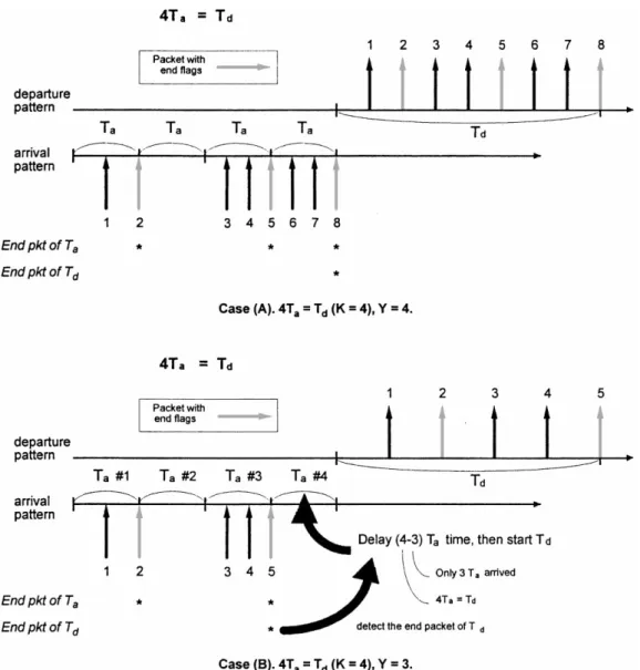
In Fig. 6, the length of Tais four times of the length of Td,
so the packets buffered within a Taframe are sent out in four
consecutive Td frames. The switch node decides which
packet to be sent out according to the group number. Packets 1 and 2 with group number 1 are sent out uniformly in the first Tdframe. As there is no packet with group number 2,
the second Tdframe is empty as shown in the figure. Packets
3, 4, and 5 with group number 3 are sent out in the third Td
frame, etc.
2.1.2.2. Changing time frames into a larger
one. Similarly, we assume K*Ta Td,K僆 N. The intermediate node not only buffers the incoming packets
until an end packet of Td arrives, but also records the
number of Taframes which have arrived since the last end
packet of Td. We assume the number is Y (Yⱕ K). When an
end packet of Td arrives, the intermediate node waits for
(K⫺ Y)* Ta time, starts a new Td frame, and sends
buffered packets uniformly within the new frame. The purpose of the waiting time (K⫺ Y)* Ta is to buffer the
arriving packets until the end of a Td frame so that the
timing of the arrival time frame is consistent with the timing of the departure time frame. Two examples are illustrated in Fig. 7 which includes two cases of 4Ta Td. As the group number is not used in changing time frames into a larger one, the group number of each packet is not displayed in Fig. 7. In case (A) of Fig. 7, the switch node found that the end packet of Td, i.e. packet 8, has arrived,
and the number of Taarrived is 4, the switch node
immedi-ately starts a Tdframe and sends out the buffered packets
within the frame. Case (B) of Fig. 7 shows the case in which the end packet of Td, packet 5, has arrived while only 3 Td
frames have arrived; therefore, the switch node waits for one extra Ta frame time and then starts a Tdframe to send out
packets.
2.2. Admission control of MCF
The admission control mechanism is exercised before the connection is set up in order to prevent the network from being overloaded. The admission test of MCF is similar to that of CF except that the time frame length of a connection can be different on each link the connection passes, and the number of packets permitted to send out on each link may also be different. For connection c with the chosen time Fig. 6. Example of changing a larger time frame to smaller time frames.
frame Tjfor output link j, its contributed load on link j will be Uj MjL= TjCj. Mjis the number of packets permitted to send on link j during one time frame from connection c, L is the number of bits in a packet, and Cjis the capacity of the link (bits/s). Hence, for connection c to be admitted into the network, the following test should be exercised on each link it passes:
Utilization test:᭙link j on the path of connection c,
X
᭙connections pass link j
Uj⬍ 1: 1
The utilization test guarantees that all links along the path are not saturated.
2.3. End-to-end delay and jitters of MCF
The end-to-end delay of a path is determined by the initial delay at the source node and by the time frame lengths of the input and output links at each intermediate node along the
path. According to the operations of the switch nodes as described in section 2.1, the queueing delay bound at switch node i is the larger value of the arrival time frame length Tai and the departure time frame length Tdi That is, delay bound at a switch node i is Max (Tai; T
i
d). Therefore, if we define D as the end-to-end delay bound, then
D Tinitial⫹
XH i1
Max Tai; Tdi ⫹ Propagation delay; 2 where H is the switch count of the path, and Tinitial is the
delay at the source node.
We define delay jitters as the maximum variation in delay experienced by packets in a single connection. For each switch node, the output traffic pattern of one connection will be reconstructed to be similar to its previous node. Hence, a similar output traffic pattern can be maintained throughout the network even if the time frame length is changed. So the jitters of the packets in MCF is between J.-H. Huang et al. / Computer Communications 22 (1999) 56–72 61
⫺TH
d and T
H
d, in which T
H
d is the departure time frame of the last switch node in the path. If we define J as the maximum jitter (jitter bound), then
J 2TdH: 3
2.4. Discussions and comparisons
MCF inherits the characteristics of CF so that the techni-ques proposed in CF such as Delay Sending and Virtual Tag [17] can also be applied in MCF. Besides, MCF provides more flexibility than CF does. Basically, MCF is a general-ized version of CF.
Changing of the time frame length of a connection can either increase the statistical multiplexing gain for the connection or reduce the jitter bound by selecting a smaller time frame at the last switch node. However, changing the time frame length sometimes introduces a longer end-to-end delay.
As MCF is non work-conserving, it results in a lower link utilization than work-conserving schemes such as
Real-Time Virtual Clock [8, 9] and Generalized Processor Shar-ing [19, 20]. However, MCF provides both delay bound and
jitter bound. Many real-time applications, particularly those that are interactive, require a bound on jitter, in addition to a bound on delay. Note that certain applications such as non-interactive television and audio broadcasting require bounds on jitter but not delay. MCF therefore satisfies the require-ment of these applications. The issue of jitter bound is not addressed in the control schemes like Real-Time Virtual
Clock or Generalized Processor Sharing.
3. Multicast connection setup for MCF 3.1. Basic concept
The connection setup procedure of the time framing strat-egy determines the time frame length for each link along the path to satisfy the end-to-end delay bound of the connection. As CF allows only one time frame length for a connection, once the routing path (or the longest path for a multicast connection) is decided, we can derive the time frame length for each link as explained in section 1.
As for MCF, the flexibility of changing the time frame length gives us more freedom to select the time frame length for each link. As the end-to-end delay in MCF is determined by the initial delay Tinitialat the source node and the time
frame length of each link as shown in Eq. (2), we discuss the relationship among Tinitialthe time frame length, and the
delay bound first.
Tinitialis the buffered time at the source node for setting the
end flags in each packet. According to the control actions of MCF at the source node, which is presented in section 2.1.1,
Tinitialmust be larger than all time frame lengths adopted by
the connection so that the framing information can be set for each packet. That is, once Tinitial is decided, the time frame
length for each link of the connection can not be larger than
Tinitial. Therefore, we should assign a large value to Tinitialso
that there is more room for the time frame length of each link to be enlarged.
However, a large Tinitial also enlarges the end-to-end
delay, which means the possible room for the time frame length to be enlarged is reduced as the required delay bound must be satisfied. That is, if Tinitial is large, the time frame
length for each link must be small in order to satisfy the requested delay bound such that the link utilization is reduced. From this point of view, Tinitiashould not be too
large.
Therefore, the computation of Tinitialin MCF is based on
the concept of equally allocating the delay bound to the source node and switch nodes, which will be explained next. Once Tinitial is decided, the time frame length for
each link can be decided. In general, there are three steps in connection setup procedure of MCF for unicast connec-tions to determine Tinitialand each time frame length:
(1) Compute the minimum time frame length that each link can provide according to the traffic pattern and the current load of the link, and calculate the best end-to-end delay that the path can support.The minimum time frame length for link i is denoted by MinTimeFramelinki. The calculation of MinTimeFramelinki is similar to that of S&G and CF and is explained briefly. The traffic specifi-cation of a connection is provided by a set of (ri, Ti) smooth parameters, which means that during any interval of length Ti, the total arrived packets of the connection have no more than riTibits. By examining the current load and the traffic pattern of the requested connection, each intermediate node can then determine the minimal frame size for the connection. The best end-to-end delay, denoted by BestTotalDelay, is computed by Eq. (2) in which MinTimeFramelinki is used for the time frame length and the term of Tinitial in the equation is replaced
by the largest value of MinTimeFramelink1, which is denoted by MaxofMinTimeFrames.That is,
BestTotalDelay MaxofMinTimeFrames
⫹XH
i1
Max MinTimeFramelinki⫺1; MinTimeFramelinki: Note that MinTimeFrames is the basic term for Tinitial.
(2) Determine the value of Tinitial. RestDelay is defined as
the difference between the requested delay bound and
BestTotalDelay; that is, RestDelay represents the amount
that can be allocated to the source node and switch nodes. We adopt the policy of equal distribution for allocating
RestDelay, so the value of Tinitial equals the basic term
MaxofMinTimeFrames plus RestDelay/SourceHopCount,
where SourceHopCount is the number of source node and switch nodes, i.e. hop count plus one.
(3) Determine the time frame length of each link.The time frame length for each link can be relaxed instead
of assigning MinTimeFramelinkito the link as long as the requested delay bound is satisfied. We call the process of enlarging the time frame length Relaxing.
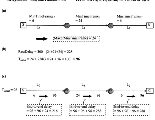
We use the example in Fig. 8 to illustrate the connection setup procedure for a unicast connection. We assume that 7 time frame sizes 3, 6, 12, 24, 48, 96, and 192 can be used for the example, and the end-to-end delay bound and jitter bound are both 300. MinTimeFramelinki of each link is shown in part (a) of the figure. Part (b) shows the
computa-tion of Tinitial, which equals Max of Min Time Frames
⫹ RestDelay=SourceHopCount 24 ⫹ (300 ⫺ (24 ⫹
24 ⫹ 24)/3) 100. Hence 96 is assigned to Tinitial. The
relaxing process for the time frame length is illustrated in part (c) of the figure. For link L0in the example, we can
enlarge its time frame length up to 96 and the end-to-end delay bound is still satisfied as shown in part (c). Relaxing of links L1and L2is similar to that of link L0.
The connection setup procedure for multicast connections J.-H. Huang et al. / Computer Communications 22 (1999) 56–72 63
Fig. 8. An example for unicast connection setup in MCF.
is a little different from that of unicast connections as there are normally more than one receiver in a multicast connec-tion. For multicast connection setup, first of all, each path from the sender to receivers is treated as an independent unicast connection, and each path computes the value of
Fig. 10. The relaxing process of the example in Fig. 9.
Fig. 11. An example of multicast connection setup in CF.
Fig. 12. The network topology for simulations.
Tinitialaccording to steps (1) and (2) mentioned above. The
value is then suggested to the sender for determining the value of Tinitialfor the multicast connection. The suggested value of Tinitialby the path from the sender to receiver R is
denoted by Suggested TinitialbyR. The sender then collects all
values of SuggestedTinitialbyRand assigns the largest value of
them to Tintialunder the constraint that the end-to-end delay
bounds of all receivers are satisfied. The relaxing process is similar to that of unicast connections.
Fig. 9 shows an example of determining the initial delay
Tinitialfor a multicast connection in MCF. We also assume
that 7 time frame sizes 3, 6, 12, 24, 48, 96, and 192 are used in the example, and the delay bound and jitter bound for all receivers are 300. MinTimeFramelinkiof each link is shown J.-H. Huang et al. / Computer Communications 22 (1999) 56–72 65
Fig. 14. Simulation result-1 for comparing MCF and CF.
in the figure. As shown in the figure,Suggested TinitialbyR1
equals MaxofMinTimeFramesR1 plus RestDelayR1/
SourceHopCountR1, i.e., SuggestedTinitialbyR1 24 ⫹ 228=3 24 ⫹ 76, so we assign 96 to Suggested TinitialbyR1. Similarly, SuggestedTinitialbyR2 48. The value of Tinitialis the largest value of Suggested Tinitial byR which does not make the end-to-end delay of all path exceed the requested delay bound. Therefore, we assign 96 to Tinitial.
The relaxing process for the example in Fig. 9 is displayed in Fig. 10. Note that the total delay of path S-R1 is computed as Tinitial ⫹ Max TimeFrameL0; TimeFrameL1 ⫹ Max TimeFrameL1; TimeFrame1; , and the total delay of path S-R2 is Tinitial ⫹ Max TimeFrameL0; TimeFrameL3 ⫹ Max TimeFrameL3; TimeFrameL4 ⫹ Max TimeFrameL4; TimeFrameL5 ⫹ Max TimeFrameL5; TimeFrameL6. Link L0is first relaxed.
Enlarging the time frame length of link L0 to 48, the
total delay of path S-R1 TotalDelayR1 becomes
96 ⫹ 48 ⫹ 24 168, and the total delay of path S-R2
becomes 96 ⫹ 48 ⫹ 48 ⫹ 48 ⫹ 24 264. If we enlarge the time frame length of link L0to 96, the total delay of
path S-R2 becomes 96 ⫹ 96 ⫹ 48 ⫹ 48 ⫹ 24 312 which violates the delay bound 300. Therefore, the final time frame length of link L0is 48.
In step (2), link L1 and link L3can be relaxed
concur-rently. Enlarging the time frame length of link L1 to 96
makes the total delay of path S-R1 288 as computed in the figure. Similarly, the time frame length of link L3can
be enlarged to 48. The relaxing process of other links is similar to that of links L0, L1, and L3 as presented above
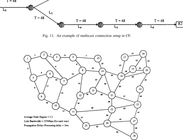
and the final time frame lengths are displayed in the figure. Applying CF, instead of MCF, to the example in Figs. 9
and 10, we can easily derive the unique time frame length of each link from the delay bound and the link count of the longest path. The time frame length using CF is displayed in Fig. 11. Comparing the final time frame length of each link by MCF in Fig. 10 with those by CF in Fig. 11, the time frame length of link L1and L2of Fig. 10 is larger than that of
Fig. 11, which shows the flexibility advantage of MCF over CF.
In the next section, the algorithm of multicast connection setup for MCF is presented in detail. The algorithm is adopted in the simulation of performance evaluation in section 4.
3.2. Algorithm of multicast connection setup
There are two steps for connection setup in MCF: (1) determining the initial delay and (2) relaxing the time frame for each switch node. The first way and the second way of connection setup determine the initial delay Tinitialof
the connection, and the third way performs relaxing. Vari-ables used in MCF are defined as follows:
[Variables used in MCF]:
DelayBound
the requested delay bound of all receivers.
JitterBound
the requested jitter bound of all receivers.
SourceHopCountR
the number of the source node and switch nodes from the sender to receiver R, i.e. hop (switch) count plus one.
Link0…linkH
the links from the sender to receiver R, where H is the Fig. 16. Simulation result-3 for comparing MCF and CF.
switch count and link0is the link between the sender and the
first switch node.
MinTimeFramelinki
the minimum time frame that link i can provide.
MaxofMinTimeFramesR
the largest value of MinTimeFramelinkion the path from the sender to receiver R.
BestTotalDelayR
the best total delay of the path from the sender to receiver R.
SuggestedTinitialbyR
the suggested value of Tintialcomputed by receiver R in the first way.
RestDelayR
the rest delay of the path from the sender to receiver R. J.-H. Huang et al. / Computer Communications 22 (1999) 56–72 67
Fig. 17. Simulation result-4 for comparing MCF and CF.
Tinitial the initial delay chosen by the sender for the
multicastconnection.
3.2.1. 1st way
1. At each receiver R, MaxofMinTimeFramesR Max MinTimeFramelinki
2. If 2·MinTimeFramelinkH⬎ JitterBound then receiver R is rejected.where linkHis the last link of the path from the sender to receiver R.
3. BestTotalDelayP R MaxofMinTimeFramsR ⫹
H
i1Max MinTimeFramelinki⫺1; MinTimeFramelinki 4. RestDelayR DelayBound ⫺ BestTotalDelayR
If (RestDelayR ⬍ 0) then receiver R is rejected.
5. SuggestedTinitialbyR MaxofMinTimeFramesR ⫹ RestDelayR=SourceHopCountR
3.2.2. 2nd way
The sender collects MinTimeFramelinki and SuggestedTinitialbyR.
The initial delay Tinitialis assigned as the largest value of SuggestedTinitialbyRunder the condition that the total
end-to-end delayⱕ DelayBound; ᭙receiver R.
3.2.3. 3rd way: [Relaxing]
We enlarge the time frame length of each link on the path according to the following three constraints in which the new time frame length of the link being relaxed is denoted by NewTimeFrame.
1. NewTimeFrameⱕ Tinitial
2. After updating the new time frame length, the end-to-end delay of the path which the link is on can not be larger than the delay bound, i.e., Tinitial⫹
PH i1
Max TimeFramelinki⫺1; TimeFramelinki ⱕ DelayBound; where TimeFramelinki is the time frame length of link i. The relaxing process continues until all links on the path are relaxed.
3. If the time frame is for the last link of the path to receiver R, then the following condition must be satisfied:
2. NewTimeFrameⱕ JitterBound 4. Performance evaluation
Some simulation results are presented in this section to compare MCF with CF in performance. The experimental environment including the network topology, the traffic model, and the way to construct a multicast tree are described next.
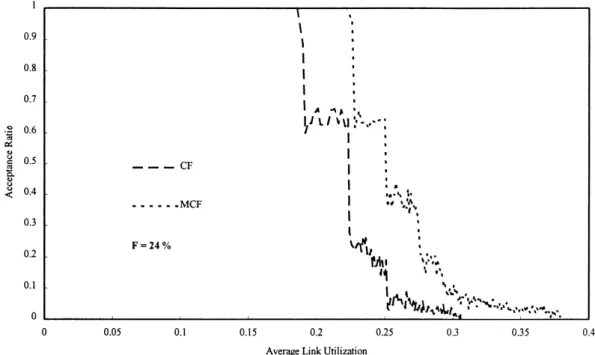
4.1. Experimental environment
The network topology used in the simulation is shown in Fig. 12 in which the average degree of node is 3.2, the bandwidth of each link is assumed to be 155 Mbps for each direction, and the bandwidth of links to the end hosts, which are not displayed in the figure, is assumed to be 620 Mbps. Note that only switch nodes are displayed in Fig. 12, and the end hosts are not displayed in the figure. We adopt the train model as illustrated in Fig. 13 to specify the traffic pattern. The traffic pattern can be described by six parameters: BusrtLength1, BurstRate1, IdleLength1,
Burs-tLength2, BurstRate2, and IdleLength2. Two sets of the
parameters, one for smooth traffic and the other for bursty traffic are used in the simulations:
1. Smooth traffic: BusrtLength1 30 ms; BurstRate1 8 KBytes=sec; IdleLength1 30 ms; BurstLength2 20 ms; BurstRate2 4 KBytes=sec; IdleLength2
20 ms:
2. Bursty traffic: BusrtLength1 20 ms; BurstRate1 48 KBytes=sec; IdleLength1 20 ms, BurstLength2 30 ms; BurstRate2 4 KBytes=sec; IdleLength2
30 ms:
The switch nodes for the sender and receivers of a multi-cast connection are randomly and uniformly selected from the 28 nodes in the network. The number of receivers is determined by the group size of the connection. Once the sender and receivers of a connection are decided, the
Short-est Path Tree (SPT) [18] algorithm is adopted to construct a
multicast routing tree for each connection. SPT algorithm in the simulation first finds the shortest delay paths from the sender to all receivers, then the algorithm combines the paths found into a multicast tree.
The packet size used in the simulation is 53 bytes and the sum of packet processing time and propagation delay on each link is assumed to be 3 ms. Each switch node selects the time frame of a connection on an output link from the following 7 time frame lengths: 3 ms, 6 ms, 12 ms, 24 ms, 48 ms, 96 ms, and 192 ms.
4.2. Simulation results and discussions
The criterion to evaluate the performance in the simula-tion is the acceptance ratio of connecsimula-tion setup requests
with respect to the corresponding average link utilization. The acceptance ratio is calculated as that the number of successful connection setup divided by the number of total connection requests. A successful connection setup requires the delay bound and jitters bound of all receivers in a connection to be satisfied. The simulation program computes and records the acceptance ratio for every 300 connection requests, and the simulation will stop when there are more than 600 consecutive connection setup requests failures. In this case, the network is defined as saturated.
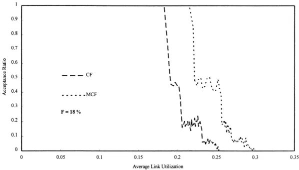
To compare MCF with CF, we define an improvement factor F as the ratio of increased link utilization of MCF over CF when the network is saturated. That is,
F
link utilization using MCF⫺ link utilization using CF
link utilization using CF :
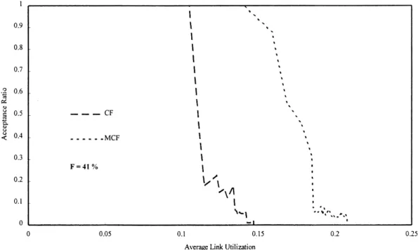
1. Figs. 14 and 15 show results of group size 2 (2 receivers) with different traffic patterns (smooth, bursty) for delay bound 300 ms and jitter bound 30 ms. Results of group sizes 4 and 8 are shown in Figs.16,17 and Figs.18,19 respectively. MCF obtains a significant performance improvement over CF when connections require a tight jitter bound (30 ms) by comparing Figs. 14–19. The reason is that the time frame length of each link on the path in CF is the same and is limited by the jitter bound, hence a small jitter bound forces the frame length to be also small and thus reduces the link utilization. Instead, J.-H. Huang et al. / Computer Communications 22 (1999) 56–72 69
only frame length of the last link of a connection path is limited by the jitter bound in MCF, and the ability of changing the time frame length releases the limitation of time frame lengths of other links on the path. There-fore, link utilization is improved significantly in MCF as shown in the simulation.
2. Figs. 20 and 21 display the simulation results of delay bound jitter bound 300 ms. From these figures, the performance improvement factor F decreases to 10% while the connection requires a looser jitter bound. By comparing the curves of MCF in Fig. 18 with that in Fig. 20 and Fig. 19 with Fig. 21, there is no significant differ-ence in the average link utilization between cases of jitter bound equals 30 ms and jitter bound equals 300 ms. However, CF obtains better link utilization in the case of jitter bound equals 300 ms than that of jitter bound equals 30 ms, since the time frame length in CF is only limited by the delay bound and the longest path instead of the jitter bound. A better link utilization of CF under a looser jitter bound implies that the jitter bound may affect the link utilization significantly, while the performance of MCF is almost not affected by a tighter jitter bound as mentioned earlier.
3. As we can see from the simulation results of smooth and bursty traffic patterns, the improvement of MCF over CF under bursty traffic, as displayed in the figures, is more significant than those under smooth traffic. The reason is that a larger time frame length can obtain more multi-plexing gain for bursty traffic pattern. Although the performance of MCF under bursty traffic also degrades, the improvement percentage of MCF over CF is increased.
4. In order to inspect the impact of hop count on the perfor-mance, we introduce the constraint of hop count for the multicast group so that the sender and receivers of a group do not spread wide over the network. More speci-fically, hop count constraint X means the sender and receivers in the same multicast group can only locate at a distance of hop count⬍ X. For example, the sender attached to switch node 1 can only have receivers attached to switches 2, 3, 5, 6, 7, 9 in Fig. 12 if X 3. Note that the hop count constraint only limits the selec-tion of sender and receivers, the path length of the final route for a multicast group may exceed the hop count constraint as the route finding algorithm tries to search for a smallest delay path from the sender to each receiver. The acceptance ratio for the case of X 3 is displayed in Fig. 22. By comparing Fig. 15 with Fig. 22, the accep-tance ratio and average link utilization in MCF under
X 3 increases much more than that without hop
count constraint. This is reasonable since more delay can be allocated to each link under the condition X 3. 5. All figures of the simulation results show that the phenomenon of sudden drop of the acceptance ratio always happens in the figures. This consequence is caused by the route finding algorithm of the simulation. The route finding algorithm tries to find a path with the minimum total delay from the sender to each receiver, and combines the paths found for all receivers. Thus when the network load is light, the acceptance ratio for connection requests is always 100% which means no connection request is rejected. Once a connection request is rejected from setting up, it is very likely that some links’ resources are almost fully allocated, and that Fig. 21. Simulation result-8 for comparing MCF and CF.
causes the network topology to be divided into several parts. The following connection requests will be rejected if the sender and receivers of the connection are located in different parts. Therefore, the acceptance ratio drops suddenly. The phenomenon of sudden degradation continues when more links get saturated and divide the network into more isolated parts until the whole network is saturated.
5. Conclusion
Considering the characteristics of multicast transmissions and the time framing strategy, MCF removes the depen-dency of the time frame lengths of links along the path of a connection by allowing the time frame length to be changeable. By so doing, simulation results show that up to 60% link utilization improvement can be achieved in some cases compared with those using only Continuous Framing strategy. Moreover, as MCF is a generalized form of CF, thus all techniques associated with CF such as delay sending and virtual tag can also be adopted by MCF to further improve the link utilization. In summary, major contributions of this article are listed below. 1. MCF provides bounded end-to-end delay/jitter and loss
free transmissions as in CF. Moreover, MCF allows changing of the time frame length such that the link utilization is increased.
2. The link utilization of MCF for connections requiring
tighter jitter bounds is enhanced even more significantly over CF as shown in the simulations. Similarly, MCF performs much better than CF when the traffic pattern is bursty.
3. MCF only introduces a small overhead during the connection setup phase and a small overhead during the data transmission phase; hence, MCF is suitable for real-time applications over high-speed networks.
References
[1] H Zhang, S Keshav, Comparison of rate based service disciplines, ACM SIGCOMM (1991) 113–121.
[2] D.D. Clark, S. Shenker, L Zhang, Supporting real-time applications in an integrated services packet network: architecture and mechanism, SIGCOMM (1992) 14–26.
[3] M. Sidi, W.-Z. Liu, I. Cidon, I. Gopal, Congestion control through input rate regulation, IEEE Trans. on Comm. (1993) 471–477. [4] C.M. Aras, J.F. Kurose, D.S. Reeves, H. Schulzrinne, Real-time
communication in packet-switched networks, in: Proceedings of IEEE, Jan. 1994, pp.122–139.
[5] A. Campbell, G. Coulson, D. Hutchison, A quality of service archi-tecture, ACM SIGCOMM (1994) 6–27.
[6] A. Demers, S. Kashav, S. Shenker, Analysis and simulation of a fair-ing-queueing algorithm, ACM SIGCOMM (1989) 1–12.
[7] C.R. Kalmanek, H. Kanakia, Rate controlled servers for very high-speed networks, GLOBECOM (1990) 30–39.
[8] L. Zhang, VirtualClock: A new traffic control algorithm for packet switching networks, ACM Computer Communications Review 12 (4) (1990) 19–29.
[9] G.X. Geoffery, S.L. Simon, Delay guarantee in virtual clock server, IEEE/ACM Trans. on Networking 3 (6) (1995) 683–689.
J.-H. Huang et al. / Computer Communications 22 (1999) 56–72 71
[10] D. Ferrari, D. Verma, A scheme for real-time channel establishment in wide-area networks, IEEE JSAC (1990) 368–379.
[11] D. Verma, H. Zhang, D. Ferrari, Guaranteeing delay jitter bounds in packet switching networks, in: Proc. TRICOMM, April 1991, pp. 35– 46.
[12] H. Zhang, D. Ferrari, Rate-controlled static-priority queueing, in: Proc. IEEE INFOCOM 1993, San Francisco, California, pp. 227–236. [13] S.J Golestani, Congestion-free transmission of real-time traffic of real-time traffic in packet networks, IEEE INFOCOM (1990) 527– 536.
[14] S.J. Golestani, A framing strategy for congestion management, IEEE JSAC 9 (7) (1991) 1064–1077.
[15] S.J. Golestani, Congestion-free communication in high-speed packet networks, IEEE Trans. on Communications 39 (12) (1991) 1802– 1812.
[16] S.J. Golestani, A stop-and-go queueing framework for congestion management, ACM SIGCOMM (1992) 8–18.
[17] B.-J. Tsaur, J.-H. Huang, Continuous framing mechanism for conges-tion control in broadband networks, Computer Communicaconges-tions 18 (10) (1995) 718–724.
[18] S. Deering, D. Estrin, D. Farinacci, V. Jacobson, C.-G. Liu, L. Wei, An architecture for wide-area multicasting routing, ACM SIGCOMM, 1994 126-135.
[19] A.K.J. Parekh, R.G. Gallager, A generalized processor sharing approach to flow control- the single node case, in: Proc. IEEE INFO-COM, 1992.
[20] A.K.J. Parekh, R.G. Gallager, A generalized processor sharing approach to flow control in integrated services networks: the multiple node case, in: Proc. IEEE INFOCOM, 1993, San Francisco, Califor-nia, pp. 521–530.