ON THE INTERACTION OF ECONOMIC DEVELOPMENT AND URBAN PLANNING: A CASE STUDY OF TAIWAN*
Chu-Chia Lin Depar tment of Economics National Chengchi Univer sity
Taipei, Taiwan, 116
I. Introduction
As a city's economy develops, more and more people get together chasing the growing job opportunities in the city. At the meantime, the demand for civil services, such as water supply, housing, transportation, hospital, school, park, etc., in the city is also increasing as population grows. In order to provide its citizens with a better living environment, the city government has to provide a profound urban planning to meet citizens’ demand. Meanwhile, the city government is the only one who could provides those civil services, since most of those goods are local public goods which private sector is usually less willing to provide. Moreover, the demand for local public goods in a city is higher and higher when residents’ income is growing. At the same time, the city government is able to provide more local public goods when its residents are richer and thus paying more taxes. Therefore, it is quite common to see a better urban planning at a city with higher household income.1
On the other hand, a well-planned urban planning will provide a more efficient usage of limited land supply of the city. It is necessary for a city with a proper zoning policy since the agglomeration effect and external effect are very significant for urban land use. For example, commercial land use is usually very condense for saving customers' travel time. In fact, agglomeration effect is essential for commercial land use. Industrial land use is another story. Industrial plants commonly generate certain negative external effects, such as noise and air pollution, thus industrial zones should be away from residential areas. Furthermore, a proper urban plan usually provides more roads and other transportation constructions, which saves travel time for its residents, goods, and services. Therefore, a proper-planed city will not only enlarge its citizens' welfare, but will also increase their income by more efficient land usage.
Though it has a strong economic reasoning for urban planning, traditional urban plans are more based on political reasons and less on economic consideration. Mills (1979) argued that most urban plannings were more as a legal issue, but not for economic incentive. Therefore, he
*Paper presented at the International Urban Development Association 22nd Annual Congress, Taipei, May 25-29,1998. The author thanks for the financial support from National Science Foundation, NSC87-2415-H-004-06.
1Tiebout (1956)'s famous model on "voting by foot" specifically talked about the impact of local government's
concluded that city government usually intends to over control urban land use, which could result in less efficient land use. Therefore, the real effect of urban planning on economic efficiency is still unclear. For example, Bailey (1959) and Babcock (1966) found that urban planning will increase the efficiency of urban land use, while Stull (1974), Ohls, Weiburg, and White (1975), and Hirsch (1984) found it is inconclusive that whether urban plan can improve efficient urban land use or not.
However, traditionally, most literature concentrates their research on the effect of zoning policy on economic development,2
because they believe that urban planning is usually exogeneously determined by local government. But, as we mentioned above, economic development should bring a strong incentive for local governments to improve their urban planning, too. Therefore, we try to examine the size of two-way effects of economic development and urban planning in this study. Traditional research on the effect of urban planning on economic growth, without considering the simultaneous effect, could provide a biased result.
II. Economic Development and Ur ban Planning
To carefully examine the real interactive effect of economic development and urban planning, a simultaneous equation model is built on the paper. In Equation (1), we assume that the ratio of planned area to total area for a city (SPLAN) is determined by government expenditure (GOVEXP), population density (POPDEN), city or county (DUMCITY), population growth rate (GPOP), and share of population living in the planned area to total population (URBPOP), and household income (HHINCOME). When a city government spends more money, it usually implies that the government is supplying more civil services and thus it is possible that the city is doing more urban planning, too. Therefore, GOVEXP should have a positive effect on urban planned areas (SPLAN).3
A city with a higher population density (POPDEN) means that it needs more civil services, too, and so a city government has to pay more attention doing urban planning to meet its citizens' requests. We conclude that POPDEN should have a positive effect on SPLAN. Comparing to counties in Taiwan, cities have been developed earlier and, with much higher population density, should have a higher ratio of planed area. A city with a higher population growth rate (GPOP) is supposed to have a higher demand for urban plan, too. If there are more population living in planned areas, it implies that planed areas are larger. Finally, household income (HHINCOME) should have a positive effect on urban planning since households with higher income have higher demand for local public goods.4
2For example, see Stull (1974), Ohls, Weiburg, and White (1975), Richardson (1978), Hirsch (1984).
3 In fact, both government expenditure and government revenue are important in determining government activities,
such as urban planning, for example see Inman (1979). However, in Taiwan, less then 50% of every city's and county's revenue is from its own revenue. In other words, more than half of a city's or county's revenue is subsidized by the central government. Therefore, how much subsidy a city or county can get is crucial in determining its government's activities. That is, government expenditure in Taiwan is more relevant to government activities than government revenue.
4This study is not aiming for analyzing determination of income in a city, but for analyzing the correlation between
household income and urban planning. One could refer Tiebout (1955) if he is interested in studying the determination of income in a city.
Equation (2) shows that household income (HHINCOME) is determined by SPLAN, GOVEXP, DUMCITY, and employment ratio (EMPRAT). We will expect that SPLAN has a positive coefficient since we assume that a city with a proper urban plan implies a more efficient usage of urban land, and so the average household income in the city would be higher. Households staying in a city with more jobs should have a higher income because it is easier for them to find jobs. Households in cities should have a higher average income than households in counties, since living standard in cities is usually higher. Finally, government expenditure is crucial for household income because a higher government expenditure implies more local jobs. So we expect that GOVEXP should have a positive coefficient.
Finally, we could write the simultaneous model as Equation (1) and Equation (2) as follow, where u1 and u2 are error terms for the two equations, respectively:
(1) SPLAN = a0 + a1*HHINCOME + a2*GOVEXP + a3*POPDEN + a4*DUMCITY
+ a5*GPOP + a6*URBPOP + u1
(2) HHINCOME =b0 + b1*SPLAN + b2*EMPRAT + b3*DUMCITY + b4*GOVEXP+u2
III. Empir ical Study
In this study, a city-level data set from Taiwan is applied to test the interaction of economic development and urban planning. We use a pooled data set where the time series is from 1975 to 1995 with 23 cities and counties in Taiwan.
The definitions of the key variables applied in this study are shown as follow:
CZONE (%): total planned commercial areas as percentage of total planed areas;
EMPRAT (%): total number of employed persons as percentage of total population;
GOVEXP (NT$1,000): average government expenditure per household;
GPOP (%): annual growth rate of total population;
HHINCOME (NT$1,000): average household income (GDP);
IZONE (%): total planned industrial areas as percentage of total planed areas;
RZONE (%): total planned residential areas as percentage of total planed areas;
SPLAN (%): total planed areas as percentage of total city area;
URBPOP (%): population in planned areas as percentage of total population;
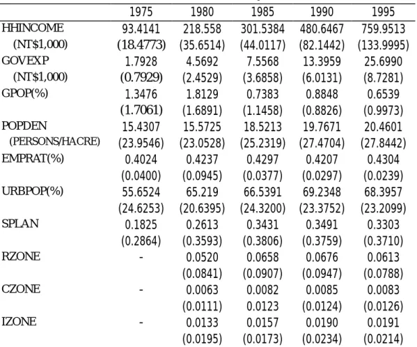
Basic statistics of the above variables for those 23 cities from 1975 to 1995 are shown at Table 1. For saving space, Table 1 shows the average figures for Taiwan as a whole for every five years. The average household annual income (HHINCOME) has increased sharply from NT$93,414 in 1975 to NT$759,951 in 1995.4
Government expenditure also goes up from NT$1,348 per household in 1975 to NT$25,699 per household in 1995. Here we see a significant phenomenon that the annual growth rate of government expenditure (11.0%) in the past twenty years is much higher than that of household income (5.8%). This phenomenon implies that the elasticity of people's demand for local public goods are greater then unit. In other words, local public goods are luxury goods by definition.
Population density (POPDEN) is also increased, but with a much slower pase, from 15.4 persons per hacre to 20.5 persons in twenty years. Employment ratio (EMPRAT) is also increasing slightly, too. As economic development, the share of population living in planed area to total population (URBPOP) in Taiwan is also increasing from 55.7% in 1975 to 68.4% in 1995. There are two reasons why the urban population share goes up quickly: First, as economic developed in Taiwan, there are more and more people moved from rural and suburban areas to urban areas. Secondly, more and more areas are included as planned areas.
The share of total planned areas to total areas in Taiwan as a whole has increased from 18.3% in 1975 to 34.3% in 1985. After 1985, the size of planned areas has not changed much till 1995. Within the planned areas, the residential area have the largest ratio, while the commercial areas have the smallest ratio.
[Put Table 1 here.]
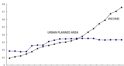
In the case of Taiwan, the total area in urban planning increases gradually as economic develops. Figure 1 shows that, as household income grows fast from 1975 to 1995, the average size of urban planning increases at the same time. Figure 1 also shows that the total size of planned areas in Taiwan was expanded fast from 1978 to 1985. On the planned areas, the shares of residential, industrial, and commercial areas are all quite stable, see Figure 2.
[Put Figure 1 and Figure 2 here.]
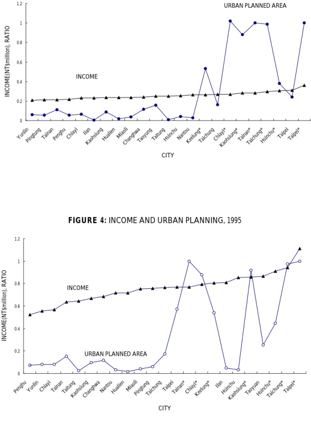
The cross-sectional data also show a positive relation of household income and the average size of urban planning. In Figure 3 and Figure 4, cities and counties are arranged by their average
household income for the year of 1982 and 1995, separately. Though the ratio of planned areas to total city areas varies among cities and counties for those two years, the figures still reveal positive correlation of income and planed areas. It confirms our hypothesis that a city with proper urban plan could generate higher income for its residents.
[Put Figure 3 and Figure 4 here.]
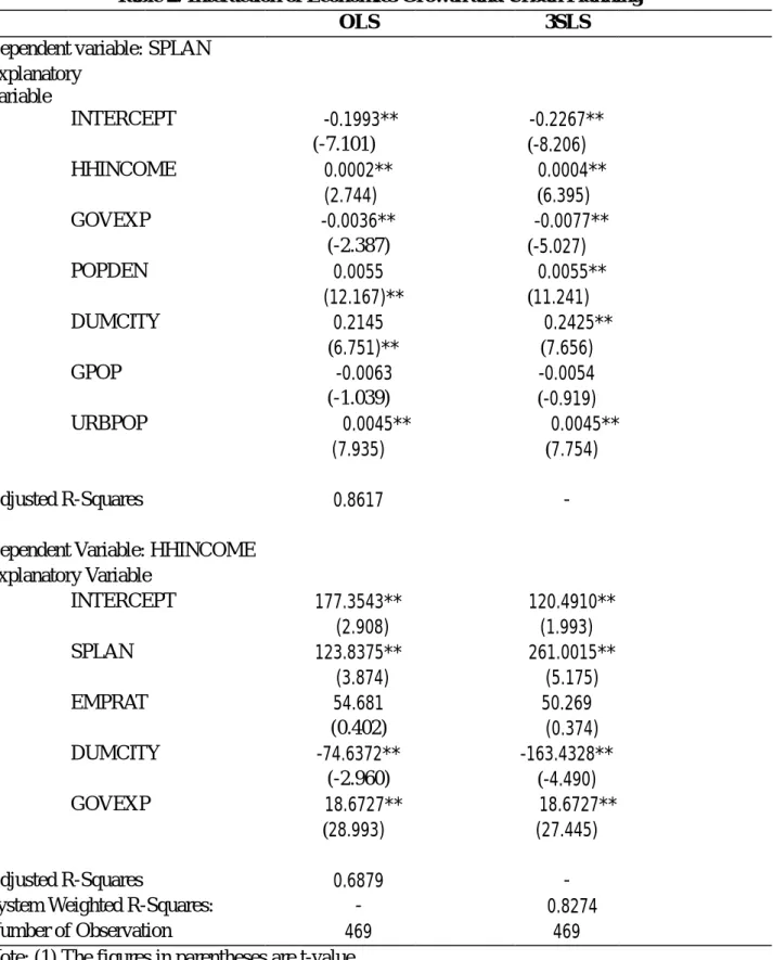
Applying a three stage least-squares estimation method (3SLS) on Equation (1) and (2) on our data set, the estimated results are shown in Table 2. Since the system weighted R-squares is 0.8274, it means that the explanatory variables could explain more than 80% of the total variation of the dependent variables. Therefore, we are quite conformable with our estimated results.
In Equation (1), we found that HHINCOME has a positive and significant coefficient (0.0004), which confirms our expectation that a city government has a strong incentive to enlarge its urban planning as its citizens' income increases. As a household's income grows, he will not only demand for a better housing condition, but will ask for a better neighborhood with more local public goods, such as school, hospital, and park. Therefore, a local government has to response for its residents’ request for urban planning with more local public goods.
Both population density (POPDEN) and urban population (URBPOP) have positive signs and are significantly different from zero, 0.0055 and 0.0045, respectively. Higher population density and more population in urban area imply more intensive demand for local public goods. Therefore, the city government also has to supply more public goods, too. DUMCITY has a positive sign (0.2425) as we expected. In fact, most cities in Taiwan have higher ratios of planned areas because cities in Taiwan have been developed earlier than counties.
Theoretically, government expenditure and urban planning should be positively correlated since a city with more government expenditure usually implies the city provides more local public goods and has more urban plannings. However, Tables 2 shows that government expenditure (GOVEXP) has a negative sign (-0.0077). One possible reason is that some local governments in Taiwan have more money on its employees' wages instead of on buying public goods. Population growth (GPOP) also has a negative sign that is inconsistent as our expectation, though it is not significant.
For the variables determining household income, Equation (2) shows that SPLAN has a positive and significant coefficient (261.0) as we expected. Again this result is consistent with our hypothesis that a proper urban plan could generate higher income for its residents. The implication of the findings is that the urban planning in Taiwan is efficient, not only on bringing up real estate prices but on enlarging average income.5
same price index, it will not change our result whether we apply a nominal figure or a real figure in this study.
Government expenditure (GOVEXP) has a positive effect on household income (18.7). It says that government expenditure does have a strong influence on local economy as we expected. Employment ratio (EMPRAT) also has a positive and significant sign (50.3) because more job opportunities mean that households have a higher average income. However, the dummy variable of city (DUMCITY) has a negative sign (-163.4), which shows that average household income in cities is lower than that in counties after controlling other relevant variables. This result is inconsistent with our expectation in that living expense in cities is usually higher than that of in counties and therefore we expect households' income in cities should be higher.6
[Put Table 2 here.]
Finally, in order to check if the interactive impacts of economic development and urban planning are significant or not, we also apply an ordinary least-square (OLS) method to estimated Equation (1) and Equation (2). The estimated coefficients are also shown in Table 2. We find that all coefficients have similar signs for both equations. The only exception is EMPRAT, from -54.7 in OLS to 50.3 in 3SLS. However, since it is not significant anyway, we don't have to worry about this coefficient too much. Though almost all of estimated coefficients have similar signs for OLS and 3SLS, the sizes of most coefficients have been changed drastically. For instance, in Equation (1), the coefficient of HHINCOME changes from 0.0002 in OLS to 0.0004 in 3SLS, while GOVEXP from -0.0036 to -0.0077. For another example, in Equation (2), the coefficient of SPLAN changes from 123.8 in OLS to 261.0 in 3SLS, while DUMCITY from -74.6 to -163.4.
The above results show that if one apply an OLS model to estimate the impact of urban planning on economic development as most traditional literature did, without considering the interactive effects of economic development and urban planning, he could get a bias result. In order to eliminate this simultaneous bias, one has to apply a simultaneous model to capture the interactive impact. Therefore, 3SLS is more suitable in this situation as this paper did.
IV. Conclusion
As a city's economy develops, more and more people get together chasing the growing job opportunities in the city. At the meantime, the demand for civil service in the city is also
(1974), they examined the impact of zoning on real estate prices. However, it is very clear in Taiwan that the real estate prices at newly planned areas are always higher than that in their neighborhoods without planning. The reason is simply because that a planned area always has better roads and other transportation constructions, and thus the real estate prices there will be higher.
6 One possible reason to explain our estimated result is that the household income we employed in this study is for a
household as a whole. Therefore, there could be certain counties with a larger average household members and thus they have a higher average household income.
increasing as population and income growing. In order to provide its citizens with a better living environment, the city government has to provide a profound urban planning to meet citizens' demand. On the other hand, a well-planned urban planning will provide a more efficient usage of its limited land supply. It is necessary for a city to have a proper zoning policy since the agglomeration effect and external effect are very significant for urban land use. Furthermore, a proper urban plan usually provides more roads and other transportation constructions which save travel time for its residents, goods, and services. Therefore, a proper-planed city will not only enlarge its citizens' welfare, but will increase their income by more efficient land usage.
To analyze the interactive impact of economic development and urban planning, this study builds up a simultaneous model to capture the interactive effect. Applying a pooling data of 23 cities and counties in Taiwan from the year of 1975 to 1995, with a three stage least-squares estimation method, this study did find that economic development and urban planning have a significant interactive effect for each other as we expected. We conclude that as an economy developed a city government has to implement more and proper urban plannings in order to meet its citizens' demand for a better living environment and for more local public goods. Moreover, a proper urban planning will not only satisfy its resident’s requests, but could generate more income for them.
Refer ence:
Babcock, R.F. (1966), The Zoning Game, University of Wisconsin Press, Madison.
Bailey, M.J. (1959), "Note on the Economics of Residnetial Zoning and Urban Renewal," Land Economics, 35, 288-392.
Block, W. (1980), "An Economic Appraisal of Zoning," in Zoning: Its Costs and Relevance in the 1980s, The Fraser Institute, Vancouver, Canada, Reprinted in S.L. Mehay and G.E. Nunn eds, Urban Economic Issues: Readings and Analysis, Chapter 10.
Evans, A.W. (1985), Urban Economics: An Introduction, Basil Blackwell Ltd.
Hirsch, W.Z. (1984), Urban Economics, MacMillan Publishing Company, New York.
Inman, R. P. (1979), "The Fiscal Performance of Local Governments: An Interpretative Review," in P. Mieszkowski and M. Straszheim eds., Current Issues in Urban Economics, Chapter 9, The John Hopkins University Press, 1979.
Mills, E.S. (1979), "Economic Analysis of Urban Land-Use Controls", in P. Mieszkowski and M. Straszheim eds., Current Issues in Urban Economics, Chapter 15, The John Hopkins University Press, 1979.
Ohls, J.C., R.C. Weisberg, and M.J. White (1974), "The Effect of Zoning and Land Value," Journal of Urban Economics, 1, 428-444.
Richardson, H.W. (1978), Urban Economics, Dryden Press, Hinsdale, Ill.
Stull, W.J. (1974), "Land Use and Zoning in an Urban Economy," American Economic Review, 64, 337-347.
Tiebout, C.M. (1955), "A Method of Determining Incomes and Their Variation in Small Regions," Papers and Proceedings of the Regional Science Association, 1, Reprinted in S.L. Mehay and G.E. Nunn eds, Urban Economic Issues: Readings and Analysis, Chapter 4.
Tiebout, C.M. (1956), "A Pure Theory of Local Expenditures," Journal of Political Economy, 64, 416-424.
Table 1: Basic Statistics: By Year 1975 1980 1985 1990 1995 HHINCOME 93.4141 218.558 301.5384 480.6467 759.9513 (NT$1,000) (18.4773) (35.6514) (44.0117) (82.1442) (133.9995) GOVEXP 1.7928 4.5692 7.5568 13.3959 25.6990 (NT$1,000) (0.7929) (2.4529) (3.6858) (6.0131) (8.7281) GPOP(%) 1.3476 1.8129 0.7383 0.8848 0.6539 (1.7061) (1.6891) (1.1458) (0.8826) (0.9973) POPDEN 15.4307 15.5725 18.5213 19.7671 20.4601 (PERSONS/HACRE) (23.9546) (23.0528) (25.2319) (27.4704) (27.8442) EMPRAT(%) 0.4024 0.4237 0.4297 0.4207 0.4304 (0.0400) (0.0945) (0.0377) (0.0297) (0.0239) URBPOP(%) 55.6524 65.219 66.5391 69.2348 68.3957 (24.6253) (20.6395) (24.3200) (23.3752) (23.2099) SPLAN 0.1825 0.2613 0.3431 0.3491 0.3303 (0.2864) (0.3593) (0.3806) (0.3759) (0.3710) RZONE - 0.0520 0.0658 0.0676 0.0613 (0.0841) (0.0907) (0.0947) (0.0788) CZONE - 0.0063 0.0082 0.0085 0.0083 (0.0111) 0.0123 (0.0124) (0.0126) IZONE - 0.0133 0.0157 0.0190 0.0191 (0.0195) (0.0173) (0.0234) (0.0214)
NOTE: The figures in parentheses are standard deviations.
SOURCE: Urban and Regional Development Statistics, Urban and Housing
Table 2: Inter action of Economics Growth and Ur ban Planning
OLS 3SLS
Dependent variable: SPLAN Explanatory Variable INTERCEPT -0.1993** -0.2267** (-7.101) (-8.206) HHINCOME 0.0002** 0.0004** (2.744) (6.395) GOVEXP -0.0036** -0.0077** (-2.387) (-5.027) POPDEN 0.0055 0.0055** (12.167)** (11.241) DUMCITY 0.2145 0.2425** (6.751)** (7.656) GPOP -0.0063 -0.0054 (-1.039) (-0.919) URBPOP 0.0045** 0.0045** (7.935) (7.754) Adjusted R-Squares 0.8617
-Dependent Variable: HHINCOME Explanatory Variable INTERCEPT 177.3543** 120.4910** (2.908) (1.993) SPLAN 123.8375** 261.0015** (3.874) (5.175) EMPRAT 54.681 50.269 (0.402) (0.374) DUMCITY -74.6372** -163.4328** (-2.960) (-4.490) GOVEXP 18.6727** 18.6727** (28.993) (27.445) Adjusted R-Squares 0.6879
-System Weighted R-Squares: - 0.8274
Number of Observation 469 469
Note: (1) The figures in parentheses are t-value.
FIGURE 1: ECONOMIC GROWTH AND URBAN PLANNING 0 0.1 0.2 0.3 0.4 0.5 0.6 0.7 0.8 1975 1976 1977 1978 1979 1980 1981 1982 1983 1984 1985 1986 1987 1988 1989 1990 1991 1992 1993 1994 1995 YEAR INCOME(NT$million),RATIO INCOME
URBAN PLANNED AREA
FIGURE 2:URBAN LAND USE
0 0.05 0.1 0.15 0.2 0.25 0.3 1979 1980 1981 1982 1983 1984 1985 1986 1987 1988 1989 1990 1991 1992 1993 1994 1995 YEAR RATIO INDUSTRIAL RESIDENTIAL TOTAL COMMERCIAL
Note: Those with * are cities and other s are counties.
FIGURE3: INCOME AND URBAN PLANNING, 1982
0 0.2 0.4 0.6 0.8 1 1.2
YunlinPingtung Tainan Penghu Chiayi Ilan
KaohsiungHualien MiaoliChanghwaTaoyungTaitung Hsinchu NantouKeelung*Taichung Chiayi*Kaohsiung*Tainan*Taichung*Hsinchu* Taipei Taipei* CITY
INCOME(NT$million), RATIO
INCOME
URBAN PLANNED AREA
FIGURE 4: INCOME AND URBAN PLANNING, 1995
0 0.2 0.4 0.6 0.8 1 1.2
Penghu Yunlin Chiayi Tainan Taitung
KaohsiungChanghwaNantou Hualien MiaoliPingtungTaichung Taipei
Tainan* Chiayi*Keelung* Ilan
Hsinchu
Kaohsiung*TaoyuanHsinchu*Taichung* Taipei* CITY
INCOME(NT$million), RATIO
INCOME