A parallel distributed processing technique for job-shop scheduling problems

Proceedings o f 1993 International Joint Conference on Neural Networks

A

Parallel Distributed Processing Technique for Job-Shop

Scheduling Problems

Chun-Chi

Lo,

Ching-Chi Hsu'

Department of Computer Science and Information Engineering

National Taiwan

University

Taipei, Taiwan

10764,

R.O.C.

Abstract

This paper presents a new parallel distributed processing (PDP) approach to solve job-shop scheduling problem which is np-complete. In this approach, a stochastic model and a controlled external energy

prove t h e scheduling solution iteratively. Different to the processing element (PE) of the Hopfield neural network model, each PE of our model represents an operation of a certain job. So, the functions of each PE are a little more complicated than that of a Hopfield PE. Under such model, each PE

is designed to perform some stochastic, collective computations. From experimental result, the solutions can be improved toward optimal ones much faster than other methods. Instead of the polynomial number

of variables needed in neural network approach, the variables number needed to formulate a job-shop problem in our model is only a linear function of the operation number contained in the given job-shop problem.

1

Introduction

Job-shop scheduling is an operation sequencing problem on multiple machines subject t o some precedence constraints among the operations. In this probelm, we have n jobs to processed through m machines. Each job must pass through each machine exactly once. We call the processing of a job on one machine an "operation". Then, there should be n

*

m operations a t all. Each job should be processed through the machines in a particular order. The order for various jobs can be different because they are assumed to be independent.

From definition [l], a schedule result is semzactzve if there does not exist an operation which could be started earlier without altering the operation sequence of each machine or violating the precedence constraints and ready dates. An optimal schedule must be semiactive and we often search solutions among the semiactive ones. But the number of semiactive schedule is (n!)" at all. This makes the search of an optimal solution very hard. Many procedures for solving job-shop scheduling problems have been introduced. They are branch and bound search method, neural network approach, interger programming technique, priority dispatching rules and many other heuristic procedures.

One example of neural network approach was presented by Foo and Takefuji [3] in which job-shop scheduling problem are mapped onto a 2-dimensional Hopfield neural netwrok model. A simulated annealing process is applied to their model in order t o avoid local minimal solutions. It suffer from some disadvantages as stated in their paper: the annealing process may take a large amount of time, and this model needs

N

=

mn(mn

+

1) number of neurons and N 2 number of interconnections.

We can see that branch and bound methods are very efficient in finding an optimal schedule while the problem size is small and the lower bound is well estimated. In another way, a combination of integer programming technique and neural network was introduced by Foo and Takefuji [4]. It can produce the scheduling result more efficiently by electronic circuit. It is very attractive in the concepts of parallel distributed processing by hardware. From our experiences and the conclusion by Foo and Takefuji [3,4], a

Correspondence author

branch and bound approach is practical for small problems, while for a large one, stochastic and mathematical approaches are suggested.

The concepts of our P D P model are similar to that of the stochastic Hopfield neural network model

[3] except that each processing element (PE) contains the information about an operation in the job-shop problem and perform a little more complicated functions. The function of every P E are identical. So we have only t o define the function that a P E must perfrom. Aided with an automatically controlled external energy, the PES will take actions cooperatively so that the schedule solutions are improved step by step.

2

The Parallel Distributed Processing Model

A PDP model processes information through the interaction of a large number of simple processing elements. In our model, each P E represents an operataion and contains the information about an operation including ready time, starting time, processing time,..etc. Through the interaction with other PES, each P E will change their own informations and the schedule result will be the final values contained in each PE.

The main ideas of our model include: (1) an automatically controlled external energy is applied t o avoid a local optimal solution, (2) each operation must try to swap the sequence order with its preceding operation on the same machine when this action is likely to eliminate the machine idle time between the processing of two adjacent operations. When the machine idle time is reduced, the total completion time of the given jobs will be also reduced. What our model does is to improve a shedule from one solution t o another better ones. Thus we will use some heuristics t o construct an initial solution and then improve the solutions iteratively toward an optimal one.

To implement the above ideas, we define the actions of each P E t o be: (1) compute the priority level

of its corresponding operation, and (2) stochastically decide whether t o swap the sequencing order with its preceding operation on the same machine according to the current scheduling result. If we swap the operations randomly, there will be little chance t o get a good or optimal schedule. If we swap the operations only when it can cause a reduction in the maximal completion time of all the jobs immediately, there will be a lot of local optimal solutions that we can never escape from it. Because of these reason, we define a heuristic for each P E to compute the priority level of its corresponding operation. An operation with higher priority level than its adjacent predecessor on the same machine will have high probability t o exchange the order with the predecessor. The priority level is determined according t o the current scheduling result. To avoid the local optimal problem, an altering external energy is used to help the search t o escape from a local optimal solution and provide the search bound of our P D P model. The external energy will increase step by step and drop t o zero when 3 conditions occur: (1) a higher energy mountain than the previous one is climbed, (2) a better solution is found and (3) no better solution is found in an large amount of iterations.

When (2) and (3) occur, the height of the energy mountain mentioned in (1) is reset to be zero. The heuristic for computing the priority level and the procedure executed in our P D P model are:

COMPUTE THE PRIORITY VALUE p l , O F OPERATION 0;

(1) The default value pl,

=

0.

(2) If the start time of some other successive operation of 0, from the precedence constraint is equal to the

finish time of o;, pl,

=

1.

(3) If the finish time of some other preceding operation of 0, from the precedence constraint is equal t o the

start time of o;, pli

=

-1.

(4) If the start time of oi is equal t o its ready time, pl;

=

-2.

(5)

oi can not move forward because of precedence constraints and the machine that 0; uses is idle in the

time before oi start, pi,

=

-2.

(6) If od is in the critical path, plj = 2.

(7) If O , meet more than one of above conditions, the later rule dominate the former ones.

PDP SCHEDULING PROCEDURE

1. Find an initial schedule solution 4 0 using some heuristic

2. Compute the energy of

40

using the function eman = energy(40) 3. ExtEnergy

=

0,StepCount

=

0 , LongCount = I(.

4. Loop until stopping conditions reached:

""-'\

i f d a t a

A

01 150 data B data

B

;

10 ,-,-.--L.

\.,--.-.-,

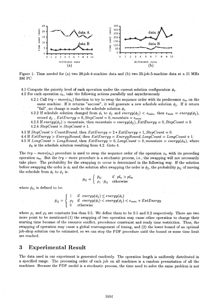
0 1 2 3 4 5 6 7 8 9 10 0 1 2 3 4 5 6 7 8 9 1 0 different runs d i f f e r e n t r u n s ( 4 (b)

Figure 1: Time needed for ( a ) two 20-job-4-machine data and (b) two 35-job-5-machine d a t a a t a 21 MHz

386 P C

4.1 Compute the priority level of each operation under the current solution configuration q5i.

4.2 For each operation on, take the following actions parallelly and asynchronously

4.2.1 Call t r y

-

move(on) function to try t o swap the sequence order with its predecessor om on the same machine. If it returns "success", it will generate a new schedule solution 4 j . If it return "fail", no change is made t o the schedule solution

&.

4.2.2 If schedule solution changed from r$i t o 4 j and energy(4,)

<

e m a n , then emin

=

energy(+j),

record

4j ,

ExtEnergy = 0,StepCount = 0 , mountain = emin.

4.2.3 If energy(q5,)

>

mountain, then mountain

=

4.2.4 StepCount

=

StepCount

+

1.

ExtEnergy = 0 , StepCount

=

0.

4.3 If StepCount

>

CountBound, then ExtEnergy = 2

*

ExtEnergy

+

1, StepCount = 0.

4.4 If ExtEnergy

>

EnergyBound, then ExtEnergy = EnergyBound, LongCount = LongCount

+

1. 4.5 If LongCount

>

LongBound, then ExtEnergy = 0, Longcount

=

0,mountain

=

energy(dk), where

4 k is the schedule solution resulting from 4.2. Goto 4.

The t r y - move(on) procedure is used t o swap the sequence order of the operation on with its preceding operation om. But the t r y

-

move procedure is a stochastic process, i.e., the swapping will not necessarily

take place. The probability for the swapping to occur is determined in the following way. If the solution before swapping the order is

4z

and the solution after swapping the order is q5j, the probability pi, of moving

the schedule from

4,

t o

4,

is:

pi, =

{

P z j

if Pin >

p1 . pz, otherwise where

pij

is defined to be:

1 if energy(q5j)

_<

energy(45)

pz if energy(4i)

<

energy(4j)

<

emin

+

ExtEnergy

{

0 otherwise

pij

=

where p1 and p2 are constants less than 0.5. We define them t o be 0.1 and 0.2 respectively. There are two more point t o be mentioned:(l) the swapping of two operation may cause other operation t o change their starting time because of the resource conflict, precedence constraint and ready time restriction. Thus, the swapping of operation may cause a global rearrangement of timing, and (2) the lower bound of an optimal job-shop solution can be estimated, so we can stop the PDP procedure until the bound or some time limit

are reached.

3

Experimental

Result

The data used in our experiment is generated randomly. The operation length is uniformly distributed in a specified range. The processing order of each job on all machines is a random permutation of all the machines. Because the PDP model is a stochastic process, the time need t o solve the same problem is not

2 5 0 .I

0 1 2 3 4 5 6 7 8 9 1 0

1 0 d i f f e r e n t data

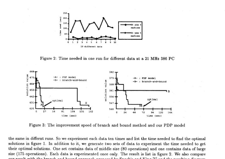
Figure 2: Time needed in one run for different data a t a 21 MMz 386 PC

582 -r -A- : PDP model -B- : branch-and-bound optimal I I _I 0 27 5 4 81 108 135 162 5 1 5

--

-A- : PDP model -B- : branch-and-bound i g optimal A i

/

5 4 0 I I I I I 0 24 40 72 96 120 1 4 4

time (sec) time (sec)

Figure 3: The improvement speed of branch and bound method and our P D P model

the same in differnt runs. So we experiment each data ten times and list the time needed t o find the optirnal solutions in figure 1. In addition t o it, we generate two sets of data t o experiment the time needed to get their optimal solutions. One set contains data of middle size (80 operations) and one contains data of large size (175 operations). Each data is experimented once only. The result is list in figure 2. We also compare our result with the branch and bound approach proposed by Spachis and King [5] and the resulting diagram is illustrated in figure 3.

4

Conclusion

For various kinds of combinatorial optimization problems, when the problem size grow up, traditional dy- namic programming, linear programming, branch and bound search and heuristic methods are very hard t o find an optimal or near-optimal solution in a reasonable time. For this sake, a parallel distributed processing model aided with some heuristic in each processing element (PE) and working through the cooperative, col- lective computation is tried to get more opportunity t o find an optimal solution in a reasonable time. From the experimental result, the PDP approach give us much encouragement of this idea. Other applications of the PDP model are being researched in our recent works.

References

[l] Simon French ,SEQUENCING AND SCHEDULING: An Introduction t o the Mathematics of the Job- [2] D.E. Rumelhart, J.L. McClelland ,Parallel Distributed Processing Volume 1: Foundations. 1986,MIT

[3] Y-P S. Foo and Y. Takefuji, ”Stochastic Neural Networks for Soving Job-Shop Scheduling: Part 1 and

[4] Y-P S. Foo and Y. Takefuji, ”Integer Linear Programming Neural Networks for Job-Shop Scheduling” [5] A. S. Spachis and J . R. King, ”Job-shop scheduling heuristics with local neighbourhood search”, Int. J .

Shop, 1982, Halsted Press. Press.

Part 2”, IEEE Int. Conf. on Neural Networks, 11-275, 1988.

IEEE Int. Conf. on Neural Networks, 11-341, 1988. Prod. Res., 1979, Vo1.17, No.6, 507-526.