A Bayesian network-based Simulation Environment for Investigating Assessment Issues in Intelligent Tutoring Systems

全文

(1)Int. Computer Symposium, Dec. 15-17, 2004, Taipei, Taiwan.. A Bayesian network-based Simulation Environment for Investigating Assessment Issues in Intelligent Tutoring Systems Chao-Lin Liu, Yu-Ting Wang, and Yu-Chih Liu Department of Computer Science, National Chengchi University, Taipei 11605, Taiwan chaolin@nccu.edu.tw the students to learn, and the most common way of assessment is asking students to answer questions in some forms of tests nowadays. It is well recognized, however, that the correctness of students’ answers does not necessarily reflect students’ competence [2]. Students might make mistakes on questions that they should be able to respond correctly, and might luckily respond to questions correctly when they do not have sufficient knowledge to do so. For simplicity of reference, these situations are often called slipping and guessing, respectively, in the literature. This uncertain relationship between students’ competence and their item-response patterns (IRP) contribute a lot to the difficulty in student assessment. (The word item carries different meanings in the literature on sub-fields of Computer Science, but it is used to represent an item of problem in a test in the literature on Education.) Educators conduct assessment activities for different purposes [22], and the most common and perceived one is to assign each testee a score. As a result, researchers have developed theories for assigning scores to testees based on testees’ item response patterns. Item Response Theory (IRT) [6] is the most dominant and widely applied theory among all alternatives, and the three-parameter IRT model considers the possibility of guessing. Although few will deny the importance of grading the testees, grading is not the only possible purpose of conducting assessment. Through the IRPs of testees, the educators may infer what teaching goals have not been achieved yet and how the educators should and could further help the testees in their learning. For instance, the IRPs allow educators to infer what concepts the testees have not really understood and what instructional material should be provided to the testees. Such applications of test results are particularly important for e-learning systems because many users adopt e-learning systems for offline and self-paced learning. For this particular reason, we consider that IRT cannot meet our demand, and we look into more details about assessment for the e-learning applications. To this end, we build a simulated assessment environment that adopts Bayesian networks [7] for capturing the uncertain relationships between the IRPs and competence levels of the testees. Using simulated students in intelligent tutoring systems (ITSs) is not new to the research community. For instance, VanLehn applies simulated students to helping people to adjust their teaching and learning strategies [18] where the models are constructed based on some reasonable cognitive analyses, e.g., [13], and Beck. Abstract - Assessment is a crucial task in develop-. ing a high quality intelligent tutoring system that can provide appropriate material to learners at the right timing. In order to explore some theoretical aspects of the assessment task, we construct a simulator that creates simulated test results of students. The simulated students may make lucky guesses in responding to questions that they are not competent enough to return correct responses, but they may also make unintentional errors on questions that they should be able to handle correctly. We cope with this uncertainty problem by incorporating Bayesian networks in the simulator. This paper elaborates on details of the simulator, and overviews experimental results of some studies that we have explored with the simulator. Experience not only indicates that this simulator is instrumental for us to explore the nature of the assessment task, but also shed light on how the simulator may be improved.. Keywords: Bayesian networks, e-learning, psychometric and educational assessment, uncertain reasoning, artificial intelligence. 1.. Introduction. As accessibility of the Internet expands with the explosive popularity of personal computers, elearning† has become a very promising complement for traditional learning channels that rely heavily on direct contacts between instructors and learners, and the number of related research work and commercial products soars accordingly. Juang’s and Tan’s groups study issues regarding e-learning in the mobile computing environment [8,15], while Kuo’s and Chen’s groups explore the applications of Webbased e-learning systems [3,9]. The teaching targets cover a variety of different topics, including English [9,15,19] and Algebra [20], and the research targets contain authoring [19,23] and delivery [10,20,23] of educational material, and assessment of students’ competence levels [10]. Instead of further covering this very broad research field, this paper concerns us with issues of assessing students in an uncertain scenario. Assessment is a key and challenging issue in education in general. Educators need to assess students’ competence so that the educators know how to help †. Although some people may insist that the term e-learning has a different connotation than the phrase intelligent tutoring, we will consider them semantically equivalent and use them interchangeably in this paper.. 234.

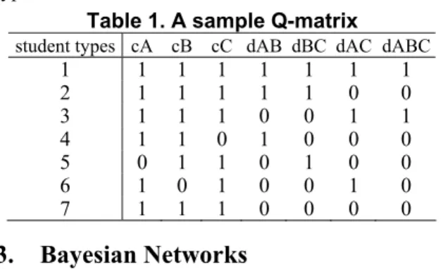
(2) Int. Computer Symposium, Dec. 15-17, 2004, Taipei, Taiwan.. in C. Let qg,c be a cell in the Q-matrix. If c represents a basic concept, then qg,c=1 signifies that the g-th type of students are competent in c. If c represents a composite concept, then qg,c=1 signifies that the g-th type of students are competent in integrating basic concepts for c. Note particularly that, when c represents a composite concept, qg,c=1 is not a sufficient condition for the g-th type of students to be competent in c. Note also that, although we use 1 or 0 in the matrix, our simulator embraces a randomization mechanism to make the relationships between student groups and competence patterns a bit uncertain, which will become clear in Section 4.1. Table 1 contains a sample Q-matrix where we assume only 7 types of students. Table 1. A sample Q-matrix. employs simulated students for locating which component in his system for improvement [1]. VanLehn refers to the simulated students as simulees, and we will continue to use this term. Researchers have admitted that simulees built on contemporary technology can mimic only limited human functions, so simulees cannot take the place of real students. However, the literature also argues that simulees are good enough for some applications and that simulees “behave” in more controllable and explainable ways such that designers of ITSs can establish more direct relationship between teaching effectiveness and simulee-dependent parameters [1,18]. We have applied the simulated system in selected ITS-related studies. We develop a mutual information-based method for adaptive item selection, and conduct a comparison study among different adaptive methods [10]. We compare some distance-based metrics, including the Euclidean and Mahalanobis distances [5], for student classification [11], and explore the possibility of mapping students’ learning processes using their IRPs [21]. Experiences collected from these studies indicate that the simulation system allows us to explore technical issues that would be impossible to achieve had we used the data collected from real students. However, we also identify weakness in the current simulator that we will enhance so that we can conduct more convincing experiments. In Section 2, we formally define the problems that we want to tackle, and, in Section 3, we quickly review the basics of Bayesian networks. We thoroughly examine the details of the simulator in Section 4, and go through the experiments that we conduct with the simulator in Section 5.. 2.. student types cA cB cC dAB dBC dAC dABC. 1 2 3 4 5 6 7. 3.. 1 1 1 1 0 1 1. 1 1 1 1 1 0 1. 1 1 1 0 1 1 1. 1 1 0 1 0 0 0. 1 1 0 0 1 0 0. 1 0 1 0 0 1 0. 1 0 1 0 0 0 0. Bayesian Networks. In the past decade or so, Bayesian networks [7] have become an important formalism for representing and reasoning about uncertainty, using probability theories as their substrate. Researchers of educational assessment have also studied the applications of Bayesian network in education [4,10]. A Bayesian network is a directed acyclic graph, consisting of a set of nodes and directed arcs. The nodes represent random variables, and each node can take on a set of possible values. The arcs signify direct dependence between the connected nodes in the applications. In addition to the graphical structure, associated with each node in the network is a conditional probabilistic table (CPT) that specifies the probabilistic relationship between values of the child and the parent nodes. By construction, the contents of the CPTs of all nodes in the network indirectly and economically encode the joint distribution of all variables in the network. As a result, we can compute any desired probabilistic information with a given Bayesian network [7].. Problem Definition. Consider the domain in which students should learn a set of concepts C={C1, C2,…, Cn}. Some of the concepts in C are basic concepts, and others are composite ones that are integrated from the basic concepts. For easier identification, we use cX and dY to denote the basic and composite concepts, respectively, where Y signifies the components that comprise the composite concept. For instance, dAB is integrated from cA and cB. We also assume that, for each concept Cj, there is a set of m(j) test items for evaluating students’ competence in Cj, and denote this set of items by Ij={Ij,1, Ij,2,…,Ij,m(j)}. For easier reference, we refer to the basic concepts of the composite concepts as the parent concepts of the composite concepts. We also refer to Cj as the parent concept of items in Ij. We classify students according to whether students are competent in what concepts in C, so there are at most 2n competence patterns. However, we assume that there are a limited number of competence patterns that the students really exhibit, and denote these types of students by G={g1, g2, …, gs}. We employ the Q-matrix that Tatsuoka [16] originally used to encode the relationships between items and concepts for representing the relationship between student types and their competence patterns. group cA dAB. dBC. cB. cC dAC. dABC. Figure 1. A sample Bayesian network Figure 1 shows a possible Bayesian network for a realizing the Q-matrix in Table 1. The group node represents the types of students. The other nodes are Boolean, each representing whether or not a student understands the concept denoted by the names of the nodes. The arcs connecting the related basic and composite concepts, e.g., those between cA, cB, and dAB, suggest that the competence of the parent con-. 235.

(3) Int. Computer Symposium, Dec. 15-17, 2004, Taipei, Taiwan.. of test items Ij for each Cj in C, and the Q-matrix. In addition to specifying these ingredients, there are more details before the simulation can better mimic the uncertainty in the real world using a Bayesian network similar to that shown in Figure 1. The current simulator allows us to specify the distribution over the student types. Since the group node is a discrete and probabilistic, simulation administrators need to specify the prior probability of each student type, i.e., Pr(group=gj) for all gj in G. For convenience, we use only 1s and 0s in specifying the Q-matrix, and take the risk of giving an illusion of our introducing deterministic relationships between the student types and their competence patterns. We compensate this by requiring the simulation administrators to specify two parameters, i.e., gSlip and gGuess, in the command files. These parameters control the probability of how students of each type will deviate from the stereotypical behaviors that are specified in the Q-matrix: gSlip controls the degree a variable will deviate from a positive value, and gGuess controls the degree a variable will deviate from a negative value. When qg,c=1 for a student type g and a basic concept c, the conditional probability Pr(c|g)‡ will be sampled uniformly from the range [1-gSlip, 1]. When qg,c=0, Pr( c |g) will be sampled uniformly from the range [0, gGuess]. At this moment, we rely on the default random number generator rand() in Microsoft Visual C++ for the sampling task. The task for creating the CPTs for the composite concepts is more complex. Recall that both types of students and competence of parent concepts of the composite concepts influence the competence of the composite concepts. Hence, if a dichotomous composite concept has k dichotomous parent concepts, the simulator must determine s×2k parameters for this composite concept. Although this is not impossible for a simulator to do so, doing so would be unnecessary. Take dAB for example. Using a logical way of thinking, a student must be competent in its parent concepts, and be able to integrate its parent concepts so that s/he can be competent in dAB. Namely, there are three main factors that simultaneously affect the student’s competence in dAB. This is clearly an example of the “AND” concept in logics, and there is an extension of it for Bayesian networks. We choose to employ “noisy-AND” nodes [7] in Bayesian networks to model composite concepts. Take the second student type in Table 1 for example. We need to obtain the influences from the basic concepts cA and cB to dAB for setting the values for Pr(dab|ca, cb ,g2). Because cA is positive, we sample the influence of cA uniformly from [1-gSlip, 1], and because cB is negative, we sample the influence of cA uniformly from [0, gGuess]. The influence of being a student in g2 will be sampled uniformly from [1-gSlip, 1] be-. cepts directly influences the competence of the composite concepts. The arcs connecting the group node and cX nodes capture the assumption that different student groups show different competence in cX, while the arcs connecting the group node and dY nodes capture the assumption that different student groups have different ability in integrating the basic concepts for a dY. Due to the page limits, Figure 1 does not include all the necessary ingredients for the problems we described in Section 2. In particular, the network does not have nodes for test items. We cannot do so because depicting nodes for all items requires a large area. If m(j)=3 for all Cj in C, we will have to add three nodes for each concept, and add links from the parent concepts to their test items. Figure 1 does not show the CPTs either, but more details about the CPTs will be provided in Section 4.1.. 4.. The Simulation Environment. Figure 2 shows major components of the simulations. Simulation administrators need to provide a command file that describes the simulation scenario. Given the command file, the simulator generates a Bayesian network that models the learning domain, and uses this network to create simulees for further applications. In our current simulations, the concept nodes are Boolean, meaning that we assume that a student is either competent or not competent in a concept. Similarly, we assume that the item nodes are dichotomous, meaning that each student responds to items either correctly or incorrectly. The final output of the simulator is a list of records of testees’ item response patterns. simulation scenario. Bayesian network generation. Bayesian network. simulee profiles. simulee generation. Figure 2. Major steps of the simulations. 4.1.. Bayesian Network-based Simulations The BNF grammar. <sim> Æ <pgroup> <concept>+ <pitem>* <params> <pgroup> Æ group-name number-of-group <subgroup>+ <subgroup> Æ subgroup-name subgroup-probability <concept> Æ <concept-type> concept-name <concept-type> Æ bconcept | dconcept <pitem> Æ item item-name parent-concept-name <params> Æ Q-matrix <p1> <p2> <p3> <p4> <p1> Æ guess value-of-guess <p2> Æ slip value-of-slip <p3> Æ gguess value-of-gguess <p4> Æ gslip value-of-gslip. This BNF grammar summarizes how we describe the setups for simulations in the command files. The semantics of the grammar will become clear in the following elaboration. As described in Section 2, major ingredients of the problems that we plan to explore include the set of student types G, the set of concepts C, and the set. ‡. This is a typical shorthand for the probability Pr(c=competent | group=g). We use c and c to denote the true and the false value of a Boolean variable, where the true value indicates competent or respond to the item correctly and the false value indicates the opposite.. 236.

(4) Int. Computer Symposium, Dec. 15-17, 2004, Taipei, Taiwan.. items are independent given a particular θ . Assume that ℑ = {i1 , i2 ,..., it } is the set of items administrated in the test. We estimate the competence Θ of testee using the following formula. Θ = arg maxθ Pr(θ | ℑ). cause a stereotypical student of g2 is capable of integrating cA and cB. After obtaining these three random numbers, we set Pr(dab|ca, cb ,g2) to their products, and Pr( dab |ca, cb ,g2) to 1- Pr(dab|ca, cb ,g2). We set the parameters for other parent configurations of dAB using an analogous method. Simulation administrators control the assignment of the CPTs for the item nodes by choosing values for slip and guess, which control the degree students make slipping and guessing, respectively. For any concept c and any of its test items, we set Pr(i|c) to a number sampled uniformly from [1-slip, 1], and Pr(i| c ) to a number sampled uniformly from [0, guess]. We then set Pr( i |c) to 1- Pr(i|c) and Pr( i | c ) to 1- Pr(i| c ).. 4.2.. = arg maxθ Pr(ℑ | θ ) Pr(θ ) = arg maxθ ∏i. Pr(i j | θ ) Pr(θ ). It should be clear that formula (2) is a realization of the naïve Bayes (NB) models that are familiar to the artificial intelligence community. Although formula (1) is more complex than typical formula used in NB models, there is no essential difference between NB models and IRT models when we use the latter for grading testees. From this perspective, we can easily see that the models we build in Section 4.1 are more complex than the IRT models. Given that we know a testee’s type, say g, the probability of correctly responding to different items, e.g. i and j, may remain dependent in our models. More specifically, unlike IRT models, the equality in (3) is not guaranteed in our models. Moreover, the equality will hold only if the parent concepts of the test items are independent given the tesstee’s identity, which generally does not hold in our simulations and in reality. Pr(i, j | g ) ? = Pr(i | g ) Pr( j | g ) (3) Hence, there are two major differences between our and the IRT models. Students are classified into types not competence levels, although we may design a conversion mechanism between these two criteria. The responses to different test items may remain dependent given the identity of the tests in our models.. Creating Simulees. Once we create a Bayesian network according to the directions given in the command file, we are ready to create simulees using the generated Bayesian network. The network in Figure 1 along with the item nodes that are not shown is one of such generated Bayesian networks, and we can easily use it to simulate how simulees respond to test items in examinations. We simulate whether a testee respond to a test item correctly or incorrectly with the help of random numbers. For a testee that belongs to the g-th student type, we can calculate the conditional probability of answering a test item i correctly, Pr(i|g), with the Bayesian network. In our simulations, we assume that testees always respond to test items, so the results of their responses must be categorized as either correct or incorrect. To this end, we sample a random number ρ uniformly from the range [0,1] to determine whether a particular testee responds to the item correctly or not. We record that the testee answers i incorrectly if ρ>Pr(i|g) and correctly otherwise. We apply a similar procedure to assign a type to each simulee. Based on the probability provided in the command file, we let each student type occupy an interval in the range of [0,1]. We sample a random number ρ uniformly from [0,1], and assign the simulee the student type whose interval includes ρ. In the simulations, we create simulees one at a time, and record their type and their IRPs in the output file. Further experiments are then conducted with the recorded data.. 4.3.. j ∈ℑ. (2). 5.. Current Applications. We have applied the simulated data in some studies on assessment-related problems. Due to the page limits, we can provide only part of the results that we observed in the individual studies, and we cannot provide detailed accounts of the studies in this paper.. 5.1.. Student Classification. As we stated in Section 1, knowing the types of testees is more useful for intelligent tutoring systems than simply grading the testees. Hence, we compare some distance-based methods for student classification [11]. More specifically, we classify testees based on Euclidean distance (ED), statistical distance (SD), and Mahalanobis distance (MD) [5] between the testees’ IRPs and the typical IRPs of different student types. In this study we rely on supervised learning [14] to learn necessary parameters from part of the simulated data (i.e., training data) for computing the distance-based similarity. We compute the degrees of similarity between the testees with unknown types (i.e., test data) and the student types based on the learned parameters for each student type. We conducted a series of experiments, and Figure 3 shows results of one experiment [11]. The horizontal axis shows that we gradually increased slipping and guessing from 0.05 to 0.25 when gGuess and. A Brief Comparison with IRT. Item Response Theory [6] is so prominent as a theory for educational assessment that we have to compare our models and IRT models. There are three IRT models, each including different factors in the model. The three-parameter model considers item discrimination ai , item difficulty bi , and the guess parameter ci . The model prescribes that a testee with competence θ will respond to item i correctly with probability provided in (1), where k i is a constant. 1 − ci Pr(i | θ ) = ci + (1) 1 + e k i ai (θ −bi ) For grading testees, it is common to assume that the probabilities of correct responses to different. 237.

(5) Int. Computer Symposium, Dec. 15-17, 2004, Taipei, Taiwan.. gSlip were both set to 0.1, and the vertical axis shows the correct rate. We can see that the correct rates decreased with the increasing chances of responding to items in unexpected manners, and, when all four parameters were 0.1, the classification error had exceeded 5%. We conjecture that, due to our relying on uniform distributions in assigning the CPTs of the Bayesian networks, the dependency among test items are not as strong as we expected, so the resulting performances of using MD and SD were not better than that of using ED. It is also possible that, even though the dependency exists, the strength of dependency is typically not very strong, and IRT should be good enough. We are currently investigating the validity of these conjectures. Accuracy. 1. is considered costly, the heuristic version of mutual information can be of help.. 5.3.. When we discuss the Bayesian network shown in Figure 1, we say that the structure is a possible way to model the Q-matrix in Table 1. The main reason for this vagueness is that there can be different ways for students to learn dABC. For instance, one may learn dABC by directly integrating cA, cB, and cC, as was indicated in Figure 1. One may also learn dABC by integrating cA and dBC as indicated in the network in Figure 5. An interesting question is that whether we can tell which network structure is used to generate the simulated data? If we can achieve this goal, we may be able to map how students learn composite concepts in the real world.. ED SD MD. 0.9. Mapping Students’ Learning Processes. group. 0.8 cA. cB. cC. 0.7 0.05. 0.1. 0.15 0.2 slip (=guess ). 0.25. dAB. Figure 3. Classification errors decrease with slip. 5.2.. BnMi DistMi BnHMi DistHMi. Accuracy. Accuracy. For computerized tests, one would like to use the least number of test items to evaluate the testees and achieve a high classification rate [17]. In previous work, we applied the simulated data to compare the classification performance achieved by different adaptive item selection criteria, and Figure 4 shows one of the experimental results [10].. 1. dAC. dABC. Figure 5. A competing structure for dABC We tried two measures for evaluating the fitness of structures to the observed IRPs [21]. The first one was based on mutual information, and the second was a heuristic stimulated by the chi square statistics. In the chart in Figure 6, we mark these two methods with M and C, respectively. Numbers “1” and “2” that are appended to both M and C, respectively, tell us whether gSlip and gGuess were set to 0.1 and 0.2. We recorded the data for the chart in Figure 6, when we actually used the structure in Figure 5 as the structure in the simulation scenario.. Adaptive Item Selection. 0.9 0.8 0.7 0.6 0.5 0.4 0.3 0.2. dBC. 6 11 16 21 Number of Administrated Items. Figure 4. Mutual information-based methods win The horizontal axis shows the number of administrated test items, and the vertical axis shows the corresponding classification rates. In this study, a number of item selection criteria were compared, but only two of them, i.e., Mi and HMi, were included in Figure 4. The curves for Mi were achieved by a selection criterion that considered exact mutual information, and the curved for HMi were achieved by a selection criterion that considered a heuristic version of mutual information. Not surprisingly, curves in Figure 4 support the intuition that we generally achieve higher classification rate if we afford to administrate more test items. The experimental results also suggest that different item selection methods lead to quite different classification rate when a limited number of test items were administrated. In particular, the mutual information-based selection criterion offered pretty good performance, and, when computing exact mutual information during the tests. 1 0.8 0.6 0.4 0.2 0 0.00. M1 C1 M2 C2. 0.05. 0.10 slip (=guess ). 0.15. 0.20. Figure 6. Finding the real structure is possible The curves in Figure 6 suggest that finding the real structure is possible when slip, guess, gSlip, and gGuess are all set to 0.1. When our system made errors, it chose the structure shown in Figure 1 most of the time. This is the kind of error that we would consider reasonable. By a closer examination of the network structures shown in Figures 1 and 5, we find that cA, cB, and cC are parent nodes of dABC, so it is easy for our system to mistakenly consider these three nodes are the direct parents of dABC rather than cA and dBC. Despite these encouraging findings, we found some cases in which it is very hard to judge the hidden structure based on the observed IRPs of testees. We have found that the contents of the Q-matrix have a great influence on the identification rates of our methods. More specifically, it is possible for us. 238.

(6) Int. Computer Symposium, Dec. 15-17, 2004, Taipei, Taiwan.. to moderately change contents of the Q-matrix but detrimentally impact the performance of our methods. The stereotypical item response patterns of student types provided in the Q-matrix and the distribution over the student types are key factors. However, we have not figured out any theoretical conclusions on this front besides these observations.. 6.. hanced environment,” ICALT’04, pp. 696-701, 2004. 9. C.-H. Kuo, D. Wible, M.-C. Chen, N.-L. Tsao, T.-C. Chou, “On the design of Web-based interactive multimedia contents for English learning,” ICALT’04, pp. 420-424, 2004. 10. C.-L. Liu, “Using mutual information for adaptive student assessments,” ICALT’04, pp. 585589, 2004. 11. Y.-C. Liu, C.-L. Liu, “Some simulated results of classifying students using their item response patterns,” TAAI’04, to appear, 2004. 12. R. J. Mislevy, R. G. Almond, D. Yan, and L. S. Steinberg, “Bayes nets in educational assessment: Where do the numbers come from?,” Proc. of the 15th Conf. on Uncertainty in Artificial Intelligence, pp. 437-446, 1999. 13. R. J. Mislevy, L. S. Steinberg, F. J. Breyer, and R. G. Almond, A Cognitive Task Analysis, with Implications for Designing a Simulation-based Performance Assessment, CSE Tech. Report 487, UCLA, USA, 1998. 14. T. Mitchell, Machine Learning, McGraw Hill, 1997. 15. T.-H. Tan and T.-Y. Liu, “The mobile-based interactive learning environment and a case study for assisting elementary school English learning,” ICALT’04, pp. 530-534, 2004. 16. K. K. Tatsuoka, “Rule space: An approach for dealing with misconceptions based on item response theory,” J. of Educational Measurement, Vol. 20, pp. 345-354, 1983. 17. W. J. van der Linden and C. A. W. Glas (eds.), Computer Adaptive Testing: Theory and Practice, Kluwer, 2000. 18. K. VanLehn, S. Ohlsson, and R. Nason, “Applications of simulated students: An exploration,” J. of Artificial Intelligence and Education, Vol. 5, No. 2, pp. 135-175, 1994. 19. C.-H. Wang, C.-L. Liu, and Z.-M. Gao. “Using lexical constraints for corpus-based generation of multiple-choice cloze items,” Proc. of the 7th IASTED Int. Conf. on Computers and Advanced Technology in Education, pp. 351-356, 2004. 20. H.-C. Wang, T.-Y. Li, C.-Y. Chang, “Adaptive presentation for effective Web-based learning of 3D content,” ICALT’04, pp. 136-140, 2004. 21. Y.-T. Wang and C.-L. Liu, “An exploration of mapping the learning processes of composite concepts,” TAAI’04, to appear, 2004. 22. D. Yan, R. G. Almond, and R. J. Mislevy, Empirical comparisons of cognitive diagnostic models, Tech. Report, Educational Testing Service, http://www.ets.org/research/dload/aera03-yan.pdf, 2003. 23. J.-T. Yang, C.-H. Chiu, C.-Y. Tsai, T.-H. Wu, “Visualized online simple sequencing authoring tool for SCORM-compliant content package,” ICALT’04, pp. 609-613, 2004.. Summary. This paper provides a detailed account of the simulator that we construct and use for generating testees’ item response patterns under some uncertain conditions. The uncertainty is a natural result of student normal behavior. The uncertainty in the simulation scenarios are captured with Bayesian networks, and the generated IRPs are used in some studies on educational assessment. Experiences indicate that the simulator is instrumental to our studies and that we may improve the simulator so that the simulation better mimic the real world.. Acknowledgements This research was supported in part by Grants 92-2213E-004-004, 93-2213-E-004-004, and 93-2815-C-004-001-E from the National Science Council of Taiwan. We thank anonymous reviewers for correcting typos in the original manuscript, and apologize for being unable to provide all requested additions as a consequence of page limits.. References In the following listing, ICALT’04 stands for Proceedings of the 4th IEEE International Conference on Advanced Learning Technologies, Joensuu, Finland, and TAAI’04 for Proceeding of the 9th TAAI Conference on Artificial Intelligence and Applications, Taipei, Taiwan.. 1. J. E. Beck, “Directing development effort with simulated students,” Lecture Notes in Computer Science 2363, pp.851-860, 2002. 2. M. Birenbaum, A. E. Kelly, K. K. Tatsuoka, and Y. Gutvirtz, “Attribute mastery patterns from rule space as the basis for student models in algebra,” Int. J. of Human-Computer Studies, Vol. 40, No. 3, pp. 497-508, 1994. 3. N.-S. Chen, Kinshuk, H.-C. Ko, T. Lin, “Synchronous learning model over the Internet,” ICALT’04, pp. 505-509, 2004. 4. C. Conati, A. Gertner, and K. VanLehn, “Using Bayesian networks to manage uncertainty in student modeling,” User Modeling and UserAdapted Interaction, Vol. 12, pp. 371-417, 2002. 5. R. O. Duda, P. E. Hart, and D. G. Stork, Pattern Classification, Wiley, 2001. 6. R. K. Hambleton, H. Swaminathan, and H. J. Rogers, Fundamentals of Item Response Theory, Sage Publications, 1991. 7. F. V. Jensen, Bayesian Networks and Decision Graphs, Springer, 2001. 8. Y.-R. Juang, Y.-H. Chen, Y.-F. Chen, T.-W. Chan, “Design of learning content development framework and system for mobile technology en-. 239.

(7)