Separation model design of manufacturing systems using the distributed agent-oriented Petri net

(1)

PLEASE SCROLL DOWN FOR ARTICLE

On: 30 October 2008

Access details: Access Details: [subscription number 731896613] Publisher Taylor & Francis

Informa Ltd Registered in England and Wales Registered Number: 1072954 Registered office: Mortimer House, 37-41 Mortimer Street, London W1T 3JH, UK

International Journal of Computer Integrated Manufacturing

Publication details, including instructions for authors and subscription information: http://www.informaworld.com/smpp/title~content=t713804665

Separation model design of manufacturing systems using the distributed

agent-oriented Petri net

Chung-Hsien Kuo; Han-Pang Huang a; Muder Jeng b; Li-Der Jeng c

a Department of Mechanical Engineering National Taiwan University Taipei 106 Taiwan. b Department of Electrical Engineering National Taiwan Ocean University Keelung 202 Taiwan. c Department of Electronic Engineering Chung Yuan Christian University Chung-Li 320 Taiwan.

Online Publication Date: 01 March 2005

To cite this Article Kuo, Chung-Hsien, Huang, Han-Pang, Jeng, Muder and Jeng, Li-Der(2005)'Separation model design of manufacturing systems using the distributed agent-oriented Petri net',International Journal of Computer Integrated Manufacturing,18:2,146 — 157

To link to this Article: DOI: 10.1080/0951192052000288215 URL: http://dx.doi.org/10.1080/0951192052000288215

Full terms and conditions of use: http://www.informaworld.com/terms-and-conditions-of-access.pdf This article may be used for research, teaching and private study purposes. Any substantial or systematic reproduction, re-distribution, re-selling, loan or sub-licensing, systematic supply or distribution in any form to anyone is expressly forbidden.

The publisher does not give any warranty express or implied or make any representation that the contents will be complete or accurate or up to date. The accuracy of any instructions, formulae and drug doses should be independently verified with primary sources. The publisher shall not be liable for any loss, actions, claims, proceedings, demand or costs or damages whatsoever or howsoever caused arising directly or indirectly in connection with or arising out of the use of this material.

(2)

Separation model design of manufacturing systems using the

distributed agent-oriented Petri net

CHUNG-HSIEN KUO, HAN-PANG HUANG

{, MUDER JENG*§ and LI-DER JENG}

{Department of Mechanical Engineering, Chang-Gung University, Tao-Yuan 333, Taiwan

{Department of Mechanical Engineering, National Taiwan University, Taipei 106, Taiwan

§Department of Electrical Engineering, National Taiwan Ocean University, Keelung 202, Taiwan

}Department of Electronic Engineering, Chung Yuan Christian University, Chung-Li 320, Taiwan

Manufacturing systems are hardly modelled and analysed in detail due to the complex and interactive behaviours of the production, movement, maintenance and dispatch on the shopfloor. In this paper, an agent-based modelling methodology is proposed to model the manufacturing systems using the separation model design approach. The agent models are constructed using the distributed agent-oriented Petri net (DAOPN). The DAOPN is a high-level Petri net (PN) and is designed based upon the coloured time Petri net (CTPN). The new designed DAOPN is especially desired to model the manufacturing systems in the separation and decomposition manners to reduce the modelling efforts and increase the modelling extensibility. The proposed DAOPN components include the immediate, pitch-type, catch-type, status-source and status-duplication places; immedi-ate, timed, decision and database-accessing transitions; and directed, inhibitor and interrupt arcs. In addition to the separation characteristics, the DAOPN can also model manufacturing systems with flexible routes of products, flexible automation of equipment, product model mixes, and huge production information intercommunication. Especially, the separation design is advantageous to the manufacturing model reconstruction and maintenance. Finally, the DAOPN is defined in this paper, and several typical applications including the production, movement, equipment failure and preventive maintenance are all discussed and evaluated.

Keywords: Distributed agent-oriented Petri net; Distributed modelling; Manufacturing system modelling; Preventive maintenance

1. Introduction

Modern manufacturing systems are becoming more competitive due to the shorter product life cycle and the fast market transition. In order to evaluate the manufac-turing systems, a practical and feasible modelling methodology is required. The Petri net (PN) (Murata 1989, Desrochers and AI-Jaar 1995, Jeng 1997, Zhou and Jeng, 1998) is one of the discrete event dynamic system

(DEDS) modelling methodologies. The PN was initially developed by Carl Adam Petri in 1962. The PN uses the mathematical and graphical representations to describe the events and conditions of the DEDS in terms of the causal relationships between events. The PN structure (Murata 1989) is a four-tuple, PN = (P, T, I, O). Where P is a ﬁnite set of places; T is a ﬁnite set of transitions; I is the input function; and O is the output functions. In a PN, conditions are modelled by places, and events are

*Corresponding author. Email: jeng@mail.ntou.edu.tw

International Journal of Computer Integrated Manufacturing ISSN 0951-192X print/ISSN 1362-3052 online_{# 2005 Taylor & Francis Ltd}

http://www.tandf.co.uk/journals DOI: 10.1080/0951192052000288215

(3)

modelled by the transitions. In general, the PN is usually used to model the concurrent and asynchronous systems, such as communications among components and manu-facturing activities.

In recent years, several studies have used the ordinary Petri net and modiﬁed Petri net to model manufacturing systems successfully. Jeng and Xie (2001) presented the modelling and analysis of semiconductor manufacturing systems with degraded behaviour using Petri nets and siphons. In this literature, the authors extended the modularly composed nets into the RCN (resource control net) merged nets to model the semiconductor manufactur-ing systems. Consequently, the state-machine modules were constructed as RCN, and an RCN merged net built the entire system successfully.

In addition, Chen et al. (2001) proposed a coloured timed Petri net (CTPN) and a genetic algorithm (GA)-based approach to model, schedule, and evaluate the wafer fabrication system. In this work, the wafer in process (WIP) status and the machine status can be completely tracked down by the reachability graph of the net. In addition, Lin and Huang (1998) used the CTPN to model the furnace behaviours of the IC fabrication. In this work, the CTPN can also emulate a quasi-environ-ment for testing and predicting the problems dynamically. Jeng et al. (1998) presented the modelling, qualitative analysis and performance evaluation of the etching area in a fab using Petri nets. In this work, the simulation

provided less than 5% error results as compared with the actual data.

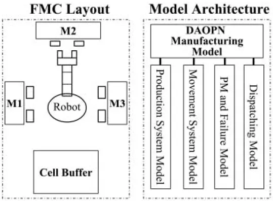
From previous PN-related research, we found that Petri nets are suitable to model the dynamic behaviours of the manufacturing systems. However, these works were not practical to model modern manufacturing systems when the behaviours of the production, movement, failure and maintenance are all considered simultaneously. The com-plicated and correlated bindings make the manufacturing models complex and unreadable. In this paper, we introduce a new type of Petri net, named DAOPN (Kuo et al. 2003). The DAOPN can increase the modelling efficiency, reduce the model complexity, and enhance the model integrability in terms of the agent technology. In particular, the agent-oriented DAOPN enables the separa-tion model design of the producsepara-tion, movement and maintenance systems. The separation design is useful in modelling and maintaining the manufacturing models. Therefore, the DAOPN manufacturing models can be separately and independently designed, and they can be seamlessly integrated. Finally, a simple flexible manufac-turing cell (FMC), as shown in figure 1, containing a robot, a parallel process machine (M1), a sequential process machine (M2) and a single process machine (M3) is modelled and evaluated using the DAOPN. The model architecture is designed as also shown in figure 1. Finally, the production, movement, failure, preventive maintenance and deadlock resolution are all discussed.

Figure 1. FMC layout and DAOPN model architecture.

(4)

2. Separation model design methodology

In modern manufacturing systems, the behaviours of production, movement, and maintenance are complex and intercorrelated. In order to model the manufacturing systems in detail, a huge model is required. However, a huge manufacturing model is hardly readable. The separa-tion model design is proposed to simplify the efforts of construction, analysis, maintenance, reconfiguration of the manufacturing models. In general, manufacturing models involve production, movement, and maintenance. Owing to the highly mixed production, the individual behaviours cannot be accurately modelled and analysed. Therefore, it is difficult to model the production, movement, and maintenance activities using a consistent modeling lan-guage.

Basically, the production behaviours include the produc-tion dispatching, product route control, tool (processing machine)/stocker capacity control, production process, etc.; the movement behaviours (Kuo et al. 2003, Kuo 2002) consist of the vehicle dispatching, vehicle collision avoid-ance, vehicle blockage-free, robot arm transport, and conveyor delivery, etc.; and the maintenance behaviours include the modelling of the mean time between failure (MTBF) and mean time to repair (MTTR) (Kuo and Huang 200).

The proposed separation modelling design approach is developed based on the distributed multi-agent coordina-tion control architecture. The agent technology (Wooldridge and Jenkins 1995, Holvoet and Verbaeten 1997) is a new and important technique in recent novel researches of the artiﬁcial intelligence (AI) area. The agent technology is deﬁned as a communicable and intelligent autonomous software component. The agent-based Petri net (Holvoet and Verbaeten 1997, Kuo et al. 2003) is used to construct the manufacturing agent models. In addition to integrating the distributed agent models, the individual agent models are capable of communicating and interacting with other agent models to perform the practical manu-facturing behaviours. The proposed model separation design concept can be characterized as follows:

1. A manufacturing system can be decomposed into the behaviours of the production, movement, and main-tenance, and these form the individual agent models. 2. The agent model is capable of autonomy, and it can operate in a stand-alone environment and evaluate itself.

3. The agent model is capable of communicability, and it can communicate with another agent models or external software components.

4. The agent model is capable of reactivity, and it can detect the environmental information and respond to it.

5. The agent model is capable of proactiveness, and it can execute the desired task.

Based on the characteristics of the agent models, the three major behaviours of the production, movement, and maintenance can be constructed and evaluated individually, and these agent models can be integrated to model the entire manufacturing behaviours based on the seamless information exchange and interaction.

3. DAOPN deﬁnitions

The DAOPN (Kuo et al. 2003) is a high-level PN, and it is designed on the characteristics of the manufacturing systems and the agent systems. In addition to modelling the processes of the manufacturing behaviours, the DAOPN enables the model’s agency to yield the character-istics of the agent model, as described in the previous section. The distributed agent-oriented Petri net (DAOPN) structure is a 13-tuple, DAOPN = (C, P0, Pp, Pc, Psrc, Pdup,

T0, Tt, Td, Tdb, Ad, Ainh, Aint). Where C is the colour set of

transitions and tokens; P0is a ﬁnite set of immediate places;

Ppis a ﬁnite set of pitch type places; Pcis a ﬁnite set of

catch type places; Psrcis a ﬁnite set of status source places;

Pdupis a ﬁnite set of status duplication places; T0is a ﬁnite

set of immediate transitions; Tt is a ﬁnite set of timed

transitions; Tdis a ﬁnite set of decision transitions; Tdbis a

ﬁnite set of database-accessing transitions; Adis a ﬁnite set

of directed arcs; Ainhis a ﬁnite set of inhibitor arcs; and Aint

is a finite set of interrupt arcs. The graphical definition of the DAOPN is shown in figure 2.

1. Place: P = {p1, p2, p3, . . . , pn}: P is a ﬁnite set of places, n4 1, including immediate place, status source place, status duplication place, pitch type place, and catch type place.

(1) Immediate place: This is defined as a container or buffer to reserve the tokens. If the reserved tokens indicate the materials, then such a place may represent the manufacturing buffer. In the manufacturing systems, the places can be used to model the conditions, buffers, and queues. (2) Status source place: The status source place is

important to the agent-oriented model design. In addition to the deﬁnition of the immediate place, the status source place deﬁnes a group of mapped status duplication places. The tokens in the status source place can be dynamically and consistently accessed by all the status duplication places. The tokens in the status source place can also be removed by the output transitions of this status source place or by the output transitions of any mapped status duplication place.

(5)

(3) Status duplication place: Each status duplica-tion place must be related to a status source place. In the DAOPN design, the status duplication place can only be the source place (hint: it is different to the status source place). Note that the source place is defined as a place that has only output arc(s). The status duplica-tion place is designed as a virtual place, and it really relates to a physical status source place. In this manner, the tokens in the status source place can be accessed at any DAOPN model consistently in terms of the invoking the status duplication places. Figure 3(a) shows a simple Petri net model, and it is impossible to divide this into several subnets using the communic-able coloured timed Petri net (CTPN) (Kuo and Huang 2000, Kuo 2002) since the tokens in P007 must be concurrently and consistently firing. In figure 3(b), nine agent models are constructed using the DAOPN, and the execu-tions of the nine models are the same as the execution of the model in (a) except for the conflict resolutions of conflict transitions. Note that places of P019 to P026 are all status duplication places, and these are mapped to the same status source place of P018.

(4) Pitch type place: This is deﬁned as the outgoing communication buﬀer of the DAOPN model. Any token arriving at the pitch type place will directly send to an assigned catch type place.

(5) Catch type place: This is deﬁned as the incoming communication buﬀer of the DAOPN model. It receives tokens from the

pitch type place. By using the pitch type and catch type places, a huge model can be divided to several sequential sub-models.

2. Transitions: T = {t1, t2, t3, . . . , tn}: T is a ﬁnite set of transitions, n4 1, including immediate transi-tion, timed transitransi-tion, decision transitransi-tion, and database-accessing transition.

(1) Immediate transitions: This is defined as the execution of the event or decision of the systems. In the DAOPN, the execution (firing) of an immediate transition may result in the changing of the entering token attributes. (2) Timed transition: This is defined as the

execution of the process that requires an elapsed time. The execution (firing) of a timed transition may also result in the changing of the entering token attributes. For example, when the timed transition represents a produc-tion process, the attributes of entering token which indicate the row material will be changed as a final product after an elapsed firing time. Note that the timed transition can handle a token at each firing time.

(3) Decision transition: The decision transition is a special case of the immediate transition. In the DAOPN, the immediate transition re-moves the tokens from its input places (with directed arc) using the rule of ﬁrst come ﬁrst serve. The decision transitions remove tokens from their input places (with directed arc) in terms of the tokens’ attributes. The token removing sequences are dynamically deter-mined by the ‘competitive token resolution rules’ as described previously.

Figure 2. DAOPN graphic deﬁnition (Kuo et al. 2003).

(6)

(4) Database-accessing transition: The database-accessing transition is designed for database-accessing the initial markings. In most Petri-net-related researches, the PN simulation models are not used to access the practical manufacturing data, since they cannot retrieve the data stored in the manufacturing execution system (MES) database. Therefore, the DAOPN develops a database-accessing transition to access the data items of the database. In this manner, the monotonic tokens can periodically ﬁre the database accessing transition, and the attri-butes (colour sets) of the transition are

updated as the attributes of the retrieved data items. Hence, the DAOPN model can be used to simulate and control the practical manu-facturing systems.

3. In a DAOPN model, the places and transitions follow the rules of P\ T = Ø, and P [ T „ Ø. 4. Colour set: The colour set of the DAOPN is deﬁned

for the places, transitions and tokens. Since the DAOPN is designed for the manufacturing systems, the colour set of the DAOPN is referred to the manufacturing attributes, such as the lot ID, lot manufacturing priority, lot commit due, OHT vehicle ID, vehicle from/to stations, vehicle current Figure 3. Status source and status duplication places.

(7)

station, and so on. When the colour set is defined for the token, the colour tokens represent the individual and identifiable manufacturing com-mands, conditions, materials, messages, and so on. When the colour set is defined to the transition, the colour sets represent the status of the facilities, decisions, identifiable events, and so on.

(1) C (pi) = {ai,1, ai,2, ai,3, . . . , ai,ui, ui =jC(pi)j};

this indicates the colour set of place pi, i= 1 to

n, where n is a non-negative integer, and j.j indicates the cardinality.

(2) C (tj) = {bj,1, bj,2, bj,3, . . . , bj,vj, vj=jC(tj)j};

this indicates the colour set of transition tj,

j= 1 to m, where m is a non-negative integer. 5. Token: The tokens reside in the places. For the DOAPN, the tokens are categorized into the monotonic token and the colour token. The monotonic token does not have any attribute value; and the attribute value of the colour token is assigned by the colour set. The colour tokens are identiﬁable. In practice, only the colour tokens can be used for control and dispatching. The graphical representation of the token is a ‘.’.

6. Input, inhibitor and output functions: The input function is defined for the directed arcs and is defined as: I (p,t)(a,b): C (p) 6 C (t) ? N; the inhibitor function is defined for the inhibitor arcs and is defined as: Inh (p,t)(a,b): C (p)6 C (t) ? N; the interrupt function is defined for the interrupt arcs, and it is defined as: Int (p,t)(a,b): C (p)6 C (t) ? N; the output function is defined for the directed arcs and is defined as: O (p,t)(a,b): C (p)6 C (t) ? N. These represent the mapping from transition t with colour b to place p with colour a, where N is a non-negative integer. Note that if these functions do not consider the colour sets, the term of ‘(a,b)’ can be ignored.

7. Marking: The marking m is used to describe the token allocations in models. The number, resided place, and colour set may change during the execution of the DAOPN. The marking of the DAOPN is an (n6 1) vector function m deﬁned as P:m (p): C (p) ? N; V p 2 P where N is a non-negative integer. Each element is denoted as m(pi)

and is deﬁned as: mðpiÞ ¼

Pui

h¼1nihaih, where nih

equalsm (pi)(aih) and is the number of tokens with

colours aihin place piat that moment; uiis the total

number of colours in place pi. m0(p) is the initial

marking.

8. Enabling and ﬁring: The transition tjis enabled with

respect to the colour bjkifm (pi)(aih)5 I(pi,tj)(aih,bjk),

V pi2 P, aih2 C(pi) andm (pr)(ars)5 Inh(pr,tj)(ars,bjk),

V pr2 P, ars2 C(pi). If piis an immediate place, then

the enabled transition tj can be ﬁred immediately.

After transition tjis ﬁred, two post conditions could

appear. For an immediate transition, the new markingm’ becomes: m’ (pi)(aih) =m (pi)(aih) + O

(pi,tj)(aih,bjk)7 I (pi,tj)(aih,bjk)

For the timed transition case, the temporary marking m’’ is: m’’ (pi)(aih) =m (pi)(aih)7 I (pi,tj)(aih,bjk)

After an elapsed time assigned in tj, the new marking

m’’’ becomes: m’’ (pi)(aih)=m’’ (pi)(aih) + O (pi,tj)

(aih,bjk)

9. Time function: This is the firing time assigned to the timed transitions, defined as f(t(bjk)), and it defines

the elapsed time required in the timed transition t associated with colour bjkto complete the ﬁring.

10. Reachability set: This consists of all reachable markings from the initial marking. A marking mn(p) is said to be reachable from the initial marking

m0(p) if there exists a sequence of ﬁrings that

transforms m0(p) to mn(p). The ﬁring sequence is

denoted ass = t1(b1k) t2(b2k). . . ts(bnk), where bjk

(j = 1 to s) is the colour set of the transition bj.

11. Safeness and boundedness: A DAOPN is said to be k-bounded or simply bounded if the number of tokens in each place does not exceed a ﬁnite positive integer k for any markingmn(p) that is reached from

a bounded initial marking m0(p). If k = 1, then a

DAOPN is said to be 1-safe or 1-bounded. 12. Liveness and deadlock: For any reachable marking,

if there exists a ﬁring sequence of transitions to reach a marking and enable transition t, then the transition t is live. A DAOPN is live if all transitions in the net are live. For any reachable marking, if there is no ﬁring sequence of transitions to make t enabled, then transition t is in a deadlock. A DAOPN is in a deadlock if there is no transition in the net to be enabled.

13. Conflict: In the DAOPN, the conflict has occurred when the number of enabled output transitions of a place is greater than or equal to 2. When conflict appears, only one transition among them can fire, and the others become disabled. In order to find the only one transition that can be fired, the DAOPN uses four rules to resolve it according to the attribute of the colour token and the transitions. The rules for resolving conflict transitions are: (1) selection of the highest priority of conflict transitions; (2) random selec-tion of conflict transiselec-tions; (3) sequential selecselec-tion of conflict transitions; (4) selection of one of the conflict transitions in terms of referring their transition names and colour sets of tokens; and (5) selection of one of the conflict transitions in terms of the meaningful token fires the higher-priority transition, and the monotonic token fires the lower-priority transition.

(8)

14. Competitive tokens: Tokens in a place compete with each other. The DAOPN develops the decision transition to resolve them. In order to determine the priority of removing tokens, the DAOPN proposes six rules to resolve it, based on the attribute-based colour sets of tokens. These are: (1) ﬁrst come ﬁrst serve (FCFS) of tokens; (2) select highest priority of tokens; (3) select from the tokens’ earliest commit due date (EDD) attributes; (4) select from the tokens’ fewest operation remaining time (FORP); (5) select from the tokens’ longest operation remaining time (LORP); and (6) select from the nearest distance attributes. Notice that the time stamp and priority are essential for the attribute-based colour set of tokens in the DAOPN.

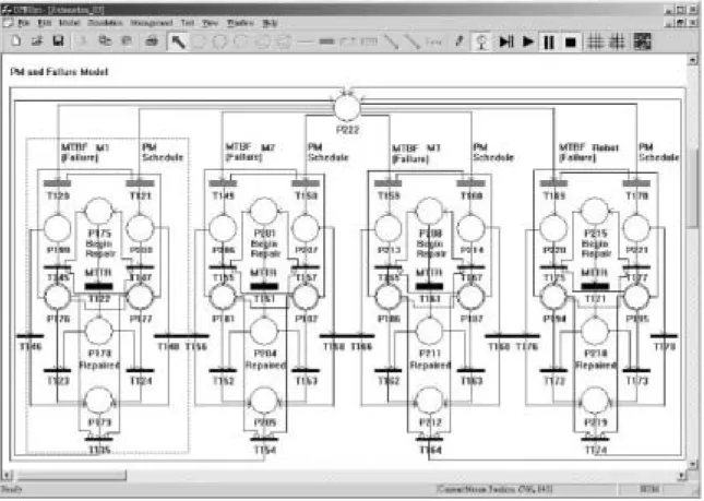
4. Modelling of failures and preventive maintenance Based on the model architecture (as shown in figure 1), four types of models are constructed separately. Initially, the equipment failure and PM schedule model is introduced, as shown in figure 4. In this paper, three process machines and one robot are discussed, and these use the same ‘net block’ but with different model parameters. A net block of a

parallel process machine (M1) is highlighted using the dashed-line rectangle. In this net block, T120 indicates the stochastic failures of M1. We use the mean time between failures (MTBF) to identify the elapsed time of this time transition. Since the failures are stochastic events, this timed transition uses the stochastic time property; T121 indicates the PM schedule of M1. We also use the mean time between failures (MTBF) to identify the elapsed time of this time transition. Since the PM schedule is pre-planned, this timed transition uses the stationary time property. T122 indicates the repair procedures. The elapsed time of T122 is set as the mean time to repair (MTTR), and it uses the stochastic time property. P176 and P177 are assigned as the status of the failure and PM activation, respectively. In particular, the introduction of the status source place makes the separation design of production and maintenance models possible. The production model that is introduced later can transparently share the failure or PM status in terms of the status duplication places. Conse-quently, when the PM (or stochastic failure) is activated, the stochastic failure (or PM) must be reset. Therefore, the interrupt arcs used here are used to cancel and interrupt the ﬁring of the others (T120 or T121). However, the interrupt arcs are used to inhibit further execution of this net block.

Figure 4. Failure and PM DAOPN model.

(9)

Finally, the individual net blocks in this model can be executed independently in terms of resolving the conﬂict transitions of P222 using the rule of ‘referring transition’s name’.

5. Modelling of production systems

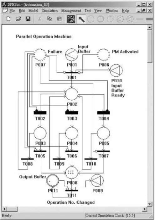
The production system is composed of the process machine and input/output buﬀers. Three types of machines, includ-ing parallel, sequential and sinclud-ingle process machines, are constructed. The agent model of the machine control model

with three parallel processes is shown in figure 5. In this model, T002 to T004 indicate three parallel processes. The elapsed times of these timed transitions are defined as the processing time, and these are determined by the route table. P001 indicates the input buffer; P002 and P008 indicate the internal buffers; P011 indicates the output buffer. Note that P011 is a status source place, and this enables the robot transport model that is introduced later to transparently share and operate the part at the output buffer in terms of the status duplication places. It also forms the separation design of the production and

move-Figure 5. Parallel process machine DAOPN model.

(10)

ment models. However, P009 and P010 are pitch-type places, and they send the messages of ‘part at output buffer can be delivered’ and ‘input buffer is available’ to the robot controller (dispatcher) model, respectively. When the process of this machine is complete, the part status is updated to the next process in terms of T011. The next process is determined using the product route. Finally, the status duplication places of P006 and P007 indicate the PM activation and failure of this machine, and these link directly to P177 and P176 in figure 4, respectively.

6. Modelling of movement system and cell buﬀers

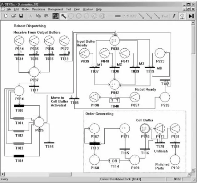
In this section, the cell buffer and material transport models are introduced. The cell buffer is shown in the bottom-right corner of figure 6. Initially, 24 parts are generated sequentially in the time period of the elapsed time set in

T113. T114 is a database-accessing transition, and it is responsible for accessing product routes and production orders. P170 and P192 are the FMC cell buffer. P170 is a status source place, and this stores the workpiece in process (WIP, unfinished parts); P192 stores the finished parts (products).

The robot controller model is shown in figure 6 excepting the dash-line encircled rectangle area. P034 to P036 and P172 receive parts from machine output buffers; P039–P041 and P223 receive input buffer ready messages from machine models. Note that the initial marking for P039–P041 is set to fit the machines’ capacity. In addition, P224–P225 and T180–T184 are used to detect and resolve the deadlock of processes due to improper location of limited machine buffers. The deadlock is resolved using the method ‘sent to cell buffer’. This can use T185 to update the ‘target buffer’ of the locked parts. In addition, T040 is a decision

Figure 6. Robot control and dispatching DAOPN model.

(11)

transition and can assign the robot control policy using the token competition rules.

The robot transport model is shown in figure 7. The upper part of this figure shows a model of checking robot arm current location. P198 is the status duplication place and indicates the PM activation of the robot. The lower part of this figure shows a model of robot transport when the robot is currently located at cell buffer. Note that the models of the robot currently located at M1, M2, and M3 (referred to in figure 1) are not shown in this paper, but they are similar to this model. In this model, P058, P065, P072 and P079 are status-duplication places and they indicate the failure of the robot. However, P052, P060, P067 and P074 are status duplication places, and they indicate the parts that stay at the machines’ output buffers and wait for delivery. Finally, the timed transition used in this model carried out the motion of ‘pickup’, ‘pick and transport’ or ‘transfer and placement’ of the robot arm. P056, P064, P071 and P078 indicate that the robot is ready, and they send a ‘robot ready’ message to the robot controller model (P057 in figure 6). P053–P055, P061–P063, P068– P070, and P075–P077 are pitch-type places, and they

send the parts to the corresponding input buﬀers of the machine model.

7. Implementation and simulation

In this paper, a simple FMC is modelled and evaluated. The DAOPN agent models are constructed using the DAOPN simulator (Kuo 2002). The DAOPN simulator is developed using the Microsoft Visual C + + , and the Microsoft SQL server is used to construct the database for storing the product route, production order, DAOPN agent model structure, initial marking, and ﬁring sequences. The DAOPN simulator provides a windows-based user-friendly DAOPN model construction and runtime simulation environment. The windows socket communication library is used to implement the activations of communication places, so that the DAOPN models can communicate with each other.

In order to evaluate the proposed agent models, a flexible manufacturing cell, as shown in figure 1, containing a parallel process machine, a sequential process machine, a single process machine, a robot arm, a cell buffer, three machine input buffers and three machine output buffers, is

Figure 7. Robot transport DAOPN model when the robot is at the cell buﬀer.

(12)

discussed. In this paper, four diﬀerent product models with distinct product routes are assigned. Each product must be processed by three machines in diﬀerent sequences, as shown in table 1. In this table, the operation number indicates the operation sequence ID, and the operation time is the processing time for each operation.

Simultaneously, to examine the modelling capacity of product mixes, four lots with different product model and different lot sizes are simulated, as indicated in table 2. In order to analyse the effects of using different control policy and maintenance, four cases are discussed, based on the above models:

1. Dispatching using FCFS rule without failure con-sideration: This condition is in terms of setting the

token competition rule as ‘FCFS’ in decision transition T (ﬁgure 6). In addition, remove all tokens in P (ﬁgure 4) in the initial marking to disable the failure and PM schedule model.

2. Dispatching using FCFS rule with failure considera-tion: This condition is in terms of setting the token competition rule as ‘FCFS’ in decision transition T (figure 6). In addition, add tokens in P (figure 4) in the initial marking to execute the failure and PM schedule model. The utilization chart for evaluating the processing/transport, maintenance and idle times for the machines and robots are summarized as shown in figure 8.

3. Dispatching using EDD rule with failure considera-tion: This condition is in terms of setting the token competition rule as ‘EDD’ in decision transition T (ﬁgure 6). In addition, add tokens in P (ﬁgure 4) in the initial marking to execute the failure and PM schedule model.

4. Dispatching using Highest Priority rule with failure consideration: This condition is in terms of setting the token competition rule as ‘Highest Priority’ in decision transition T (ﬁgure 6). In addition, add tokens in P (ﬁgure 4) in the initial marking to execute the failure and PM schedule model.

Table 1 Simulated product routes with four diﬀerent product models. Product ID Operation number Operation time (min) Machine ID PROD_1 100 0.75 M1 PROD_1 200 0.13 M2 PROD_1 300 0.35 M3

PROD_1 1000 0 Cell buﬀer

PROD_2 100 0.40 M3

PROD_2 200 0.18 M2

PROD_2 300 0.75 M1

PROD_3 100 0.12 M2

PROD_3 200 0.68 M1

PROD_3 300 0.33 M3

PROD_4 100 0.14 M2

PROD_4 200 0.34 M3

PROD_4 300 0.60 M1

Note: Simulation time unit: minute

Table 2. Simulated production orders.

Product ID Manufacturing priority Commit due Lot size Lot issue quantity PROD_1 3 100 6 1 PROD_2 5 80 8 1 PROD_3 8 70 4 1 PROD_4 6 90 6 1

Note: Simulation time unit: minute

Figure 8. Utilization chart for evaluating the processing/transport, maintenance and idle.

(13)

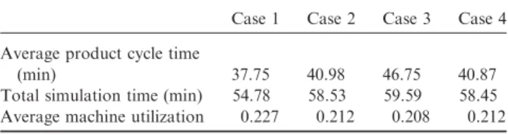
The simulation results can be evaluated based on the average product cycle time, total simulation (completeness of all assigned jobs), and average machine utilization, and they are summarized in table 3. The simulation results show that the control policy aﬀects the system performance, and the eﬀects of failure and PM cannot be ignored. Conse-quently, the dispatching rules of ‘Highest Priority’ and ‘FCFS’ perform better in these cases.

8. Conclusions

In this paper, the agent-oriented DAOPN models are constructed to achieve the separation model design of the production, movement, control and maintenance beha-viours in modern manufacturing systems. The separation model design is beneﬁcial to the construction, reconstruc-tion, maintenance, and extension of manufacturing system models. The DAOPN agent models can be designed separately and independently, and they are seamlessly integrated to perform an entire manufacturing system model. Finally, a simple FMC was modelled and evaluated for the demonstration of constructing separation models using the DAOPN. The results of using diﬀerent control/ dispatching policy are evaluated based on the product cycle times and machine utilizations with the maintenance considerations. In the future, the DAOPN and the proposed separation model design approach can be used to model more complex manufacturing systems such as the semiconductor manufacturing systems for practical appli-cations.

Acknowledgement

This research was partially supported by the National Science Council in Taiwan through Grant NSC 90-2212-E-182-009 and NSC 91-2212-E-182-002.

References

Chen, J.H., Fu, L.C., Lin, M.H. and Huang, A.C., Petri-net and GA-based approach to modeling, scheduling, and performance evaluation for wafer fabrication. IEEE Trans. Robot. Autom., 2001, 17(5), 619–636. Desrochers, A.A. and AI-Jaar, R.Y., Applications of Petri Net in

Manufacturing Systems—Modeling, Control, and Performance Analysis, pp. 55–170, 1995 (IEEE Press, Washington, DC).

Holvoet, T. and Verbaeten, P., Using agent for simulation and implementation Petri net, in Proceeding of 11th Workshop on Parallel and Distributed Simulation, Lockenhaus, Austria, 1997, pp. 134–137. Jeng, M.D., Xie, X. and Chou, S.W., Modeling, qualitative analysis, and

performance evaluation of the etching area in a IC wafer fabrication system using Petri net. IEEE Trans. Semicond. Manuf., 1998, 11(3), 358–373. Jeng, M.D., A Petri net synthesis theory for modeling ﬂexible

manufactur-ing systems. IEEE Trans. Syst. Man Cybern. B, 1997, 27(2), 169–183. Jeng, M.D. and Xie, X., Modeling and analysis of semiconductor

manufacturing systems with degraded behavior using Petri nets and siphons. IEEE Trans. Robot. Autom., 2001, 17(5), 576–588.

Kuo, C.H., Wang, C.H. and Huang, K.W., Behavior modeling and control of 300 mm fab intrabays using distributed agent oriented Petri net. IEEE Trans. Syst. Man Cybern. A, 2003, 33(5), 641–648.

Kuo, C.H., Modeling and performance evaluation of an overhead hoist transport system in a 300 mm fab. Int. J. Adv. Manuf. Technol., 2002, 20(2), 153–161.

Kuo, C.H. and Huang, H.P., Failure modeling and process monitoring for ﬂexible manufacturing systems by using colored timed Petri net. IEEE Trans. Robot. Autom., 2000, 16(3), 301–312.

Lin, S.Y. and Huang H.P., Modeling and emulation of a furance in IC fab based on colored-timed Petri net. IEEE Trans. Semicond. Manuf., 1998, 11(3), 410–420.

Murata, T., Petri nets: properties, analysis and applications. Proc. IEEE, 1989, 77(4), 541–580.

Wooldridge, M. and Jenkins, M.R., Intelligent agents: theory and practice. Knowl. Eng. Rev., 1995, 10(2), 115–152.

Zhou, M.C. and Jeng, M.D., Modeling, analysis, simulation, scheduling, and control of semiconductor manufacturing systems: A Petri net approach. IEEE Trans. Semicond. Manuf., 1998, 11(3), 333–357.

Table 3. Performance evaluations for four cases.

Case 1 Case 2 Case 3 Case 4 Average product cycle time

(min) 37.75 40.98 46.75 40.87

Total simulation time (min) 54.78 58.53 59.59 58.45 Average machine utilization 0.227 0.212 0.208 0.212 Note: Simulation time unit: minute