WiMAX網路上傳具品質服務保證之公平排程機制

(1)

國

立

交

通

大

學

資訊科學與工程研究所

碩

士

論

文

WiMAX 網路上傳具品質服務保證之公平排程

機制

Fair Scheduling with QoS Guarantees for Uplink

Transmission in WiMAX Network

研究生：詹林峰

指導教授：趙禧綠助理教授

(2)

Abstract

IEEE 802.16 Broadband Wireless Access (BWA) Network supports classes of

traffic with differentiated Quality of Service (QoS). However, the detailed of how to

schedule traffic are left unspecified. While in some recent studies, traffic scheduling

performs Strict Priority Scheduling (SPS). And the priority order is followed as

UGS>rtPS>nrtPS>BE. While in this scheduling method, starvation of lower priority

traffic will happen. The proposed scheduling algorithm is designed in purpose of

fairness improvement. We propose a new scheduling algorithm called Two-Tier

Scheduling Algorithm (2TSA). The first tier is category-based and the second tier is

weight-based. Both tiers are implemented at BS. The first tier classifies all

connections into three categories, Satisfied, Unsatisfied, and Over-satisfied. The

second tier calculates weights of each connection differently in each category and

performs bandwidth allocation. The simulation result shows that our proposed

(3)

摘要

在 IEEE 802.16 無線寬頻網路中，依據不同的品質服務保證需求定義出了各種不同的服務類型。然而，在最新的 IEEE 802.16 標準中，如何來排程不同的服務類型並沒有明確被定義，而在某些現有的研究當中，採用了一種嚴格優先權式排程，也就是當完成了高優先權的類型頻寬配置後，如果還有剩餘的頻寬時，才執行低優先權的服務類型之頻寬配置。如果用此方法來排序頻寬配置先後，將會造成低優先權的服務類型因為遲遲得不到頻寬配置，或者頻寬皆被高優先權的服務類型所佔據，而發生飢餓現象。為了改善這種不公平的現象發生，本篇論文提出了一個新的機制，＂雙層式排程演算法＂，來提升頻寬配置的公平性，也確保了品質服務保證的特性。在此改良的機制當中，第一層實作了服務串流的分類，分別依據各個串流的滿足程度來分類，可分成＂未滿足＂，＂已滿足＂，和＂過度滿足＂三種。而第二層的機制用來計算各個不同的串流在不同的類別當中所代表的權重，並且實作了頻寬配置。在模擬結果中，可證明不僅品質服務保證能夠確保，而且改善了頻寬配置的公平性。

(4)

致謝

歲月如梭，兩年的實驗室研究生涯，在這本論文完成之際，也即將劃下了休止符。從當初懵懵懂懂且出乎意料地以低空飛過之錄取分數進入這個窄門，到現今能夠獨立完成屬於自己的創作，在自感欣慰之餘，心中更是有無限的感激。回想起第一次和指導教授見面的光景，她以親切且輕鬆的態度相待，不僅加深了對教授的印象，更是下定了想要在此實驗室渡過接下來兩年的決心。在這接近八百個研究歲月的日子當中，一開始對於一個沒有網路知識背景的人來說，算是格外地吃力，想當初定期的實驗室團體討論，有如鴨子聽雷像是旁觀者般地看著其他同學和教授熱烈地討論並提出意見，腦子卻只能停留在努力吸收那些基本定義的階段。「起步比別人慢，但是進步的速度不能比別人慢」，每當遇到瓶頸或是無助的時候，屢屢想起教授這句令人深省的話。總是願意從頭講起，且不厭其煩地帶領我發覺問題的核心，讓一個原先畏懼網路專業名詞的人，變成願意為了微小的問題，難解的公式而焚膏繼晷且樂在其中的「研究生」。這種實事求是，打破砂鍋也要追根究底的態度，是這兩年來從教授身上得到最無價的收穫。實驗室同窗在這段時間當中不斷地傾囊相授與相互鼓勵，這份感動更是讓人點滴在心頭。甚至有些時候，把他人的研究當作有如自己研究般地絞盡腦汁。在彼此腦力激盪之下，也總能夠迸出來令人驚奇的結論。因此，能夠完成本篇論文，一半以上的功勞要歸功於朝夕相處的同窗以及一路上拉拔提攜的教授。在這兩年逝去的歲月裡，從睡眠不足的倦容，與缺少歡樂的日子中，換來的除了是滿滿的知識寶藏之外，更是為了研究永不放棄的精神。這股精神，在研究領域甚至在畢業後的人生大道上，將會是受用無窮。最後，感謝一路上能夠伴我同行的家人。二十多年來，從父母那原先烏黑的青絲漸成雪白的雙鬢，深感養育恩情之深，只能盡心盡力做好每一件事，來加以回報。另外，在千里之外的家姐更是時常透過越洋電話，彼此相互勉勵和打氣，能夠完成此論文，再次感謝生命中幫助或照顧過我的人。

(5)

List of Figures

Figure 1-0: Illustration of PMP topology………...1

Figure 1-1: Frame structure………4

Figure 1-2: DSA message flow BS-initiated...………5

Figure 1-3: DSA message flow- SS- initiated...5

Figure 1-4: Modulation diagram of BS and SS ...6

Figure 1-5: SPS bandwidth allocation………..14

Figure 2-1: Proposed structure...19

Figure 2-2: Flow chart of 2TSA………...23

Figure 3-1: Poisson distribution...27

Figure 3-2: Average throughput in Scenario I ...31

Figure 3-3: Fairness degree in Scenario I ...31

Figure 3-4: Average delay in Scenario I ...32

Figure 3-5: Average throughput in Scenario II-Case 1 ...36

Figure 3-6: Average throughput in Scenario II-Case 2 ...36

Figure 3-7: Fairness degree in Scenario II-10 seconds ...37

Figure 3-8: Fairness degree in Scenario II-100 seconds ...38

Figure 3-9: Average delay in Scenario II- case 1 ...39

(8)

List of Tables

Table 1-1: Bandwidth Request header fields……….7

Table 1-2: QoS parameters for each connection………8

Table 3-1: Simulation parameters……….26

Table 3-2: Throughput of rtPS in 2TSA Scenario I……….….……32

Table 3-2: Throughput of nrtPS in 2TSA Scenario I………33

Table 3-2: Throughput of BE in 2TSA Scenario I…..……….….……33

Table 3-2: Throughput of rtPS in 2TSA Scenario II……….….……...40

Table 3-2: Throughput of nrtPS in 2TSA Scenario II………...……….….…..40

(9)

Chapter 1. Introduction

WiMAX (Worldwide Interoperability for Microwave Access) is a new network architecture providing high data rate wireless transmission. Undoubtedly most of the network users are benefited with the wireless local area network (WLAN). As long as staying in an environment having access point, users can freely access the internet and communicate with the whole world. However, WiFi (WLAN) can only provide users the ability to use wireless device indoor or close to the access point. It cannot support the connection from Access Point to the Base Station of the ISP (Internet Service Provider). In recent deployment of high speed transmission between local AP and the Base Station, DSL and cable modem are playing an important role. But they are both wire line based connections. With the invention of WiMAX, the last mile broadband wireless can be achieved. The previous wire line based system established between users and ISP base stations can be replaced with microwave access deployment.

(10)

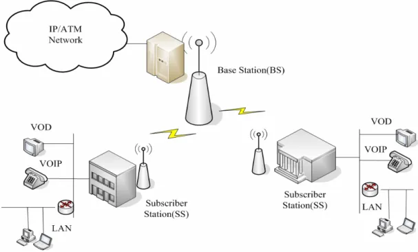
WiMAX in IEEE standard is defined as IEEE 802.16, which is also named as broadband wireless access (BWA). Two kinds of topology are currently supported, the PMP (Point-to- multipoint) topology and the mesh topology. In PMP topology, similar with traditional IEEE 802.11 WLAN, there is a central supervisor called Base Station (BS) playing the role as Access Point in WLAN and several Subscriber Station (SS) as mobile stations in WLAN. The BS supervises all the transmission of SSs. It is also be responsible for the admission control of all the SSs. And SS cannot communicate with another SS directly without BS. In mesh topology, SS can communicate and connect with another SS directly. It is just like the difference between infrastructure mode and Ad hoc mode in WLAN. Fig 1-0 [3] shows the relationship between PMP architecture and the WLAN. In IEEE 802.16 current definition, the transmission range can be up to 30 miles, transmission rate up to 130 Mbps. It can do a great help to network users especially when they are in outdoors. The users will be expected to save a great amount of cost in deploying the underground cables or extensive infrastructures. On the other hand, wireless systems have the capabilities to remain connections while the user or the device is moving. That is to say, the wireless network outperforms wired network in many aspects, as long as it can provide the same high rate transmission as in wired network. Through the integration of WiFi and WiMAX, human beings can be benefited with those advantages mentioned above.

1.1 WiMAX Background Overview

As mentioned in the first chapter, there are two topologies of WiMAX. The following contents of the thesis will all focus on the PMP topology and will have no discussion relating to the mesh topology. The communication path between BS and

(11)

SS has two directions: Uplink and Downlink. In order not to be interrupted by each other, the two directions have to be separated, multiplexed either by TDD (Time Division Duplex) or FDD (Frequency Division Duplex). FDD mode allows uplink and downlink transmits data at the same time. Owing to the frequency domain is separate, the collision or the signal interference problem can be prevented. While in TDD mode, the transmission of both directions is in the same frequency domain. Unless the transmission time is divided is there transmission error happened. And the scope of content is all covered with TDD mode especially under uplink transmission. In IEEE 802.11, the protocol defines DCF and PCF to coordinate channel access. Similar with the PCF, IEEE 802.16 PMP defines that BS coordinates and supervises all the transmission of SSs. And all the SS is ordered to obey the transmission time defined by BS. Several schemes defined to manage BS and SS has shown below:

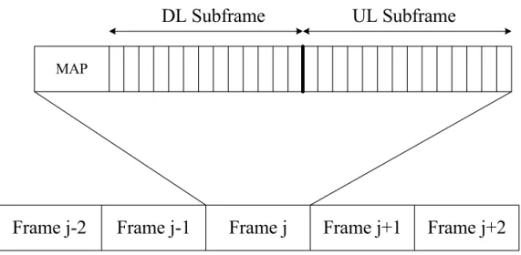
1.1.1 Frame

Structure

The unit of transmission time is named as a “frame”. Each frame consists of several physical slots (PS) just as in Fig.1-1 .BS will broadcast MAP to SSs before each frame. During Downlink (DL) Subframe, BS broadcasts data to all SSs, and each SS picks the data in the specific duration of slots defined by DL-MAP. In Uplink (UL) Subframe, the BS determines the start time and number of slots for each SS to transmit, and this information is broadcasted by the BS through UL- MAP.

(12)

MAP

UL Subframe

DL Subframe

Frame j

Frame j-1

Frame j-2

Frame j+1

Frame j+2

Figure 1-1: Frame structure

1.1.2 Connection

Identifier

In IEEE 802.16 Std[1], it defines the protocol is connection oriented. The application must establish the connection with BS, and each connection stands for one service flow. In order to identify the difference of each service flow, standard defines a 16- bit value that acts as identifier, called Connection ID (CID). During the entry and initialization every SS is assigned up to three dedicated CIDs for the purpose of sending and receiving control messages. These connection pairs are used to allow differentiated levels of QoS to be applied to the different connections carrying MAC management.

1.1.3 Service Flow Creation

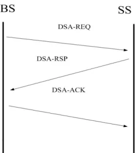
Creation of service flows may be initiated either by BS (mandatory capability) or by SS (optional capability). And there are two types of messages being responsible for the service flow creation and change. One is DSA (dynamic service addition) and the other one is DSC (dynamic service change). DSA and DSC just perform the same

(13)

function except one is in the initial of connection and the other one is during the connection status changes. The Fig.1-2 illustrates the SS- initiated and Fig.1-3 illustrates the BS- initiated. Parameters of service flows can be informed to the BS through DSA and DSC.

Figure 1-2: DSA message flow BS-initiated

(14)

Figure 1-4: Modulation diagram of BS and SS

1.1.4 Bandwidth

Request

Message

Bandwidth Request (BR) will be sent out for each flow to indicate the size of bandwidth it needs to uplink in the following frame. Then the BS determines this request to be approved or not. All BRs from the services are classified by the connection identifier based on CID and its service type, just as shown in Fig.1-4 [6]. A request may come as a stand-alone bandwidth request header or it may come as a Piggyback Request. And it is optional for each connection to use Piggyback based bandwidth request. A connection can detect the data size they need to uplink and then calculate how many time slots they are required. Once BS permits its request, it will inform that connection the specific time slots to transmit. BR may be incremental or aggregate [1]. When the BS receives an incremental BR, it shall add the quantity of bandwidth requested to its current perception of the bandwidth needs of the connection. When the BS receives an aggregate BR, it shall replace its perception of the bandwidth needs of the connection with the quantity of bandwidth requested. The

(15)

type field in the BR header indicates whether the request is incremental or aggregate.

Table 1-1: Bandwidth Request header fields

Name Length(bits) Description

BR 19 Bandwidth Request. The number of bytes of uplink bandwidth requested by the SS. The BR is for the CID.

CID 16 Connection Identifier

EC 1 Always set to zero, means no encryption

HCS 8 Header Check Sequence

HT 1 Header Type=1

Type 3 Indicates the type of BR header

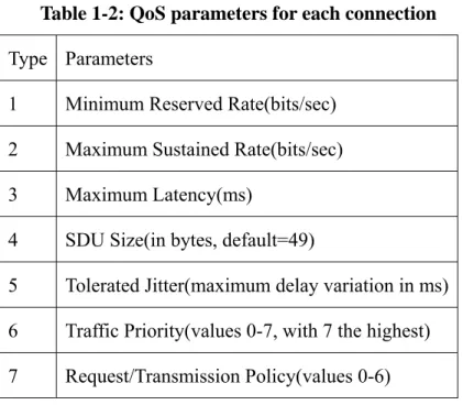
Piggybacked BR shall always be incremental. Table1-1 illustrates the BR’s header. In the type field of BR header, “000” for incremental and “001” for aggregate. Besides Piggyback for BR, stand-alone BR can be “polling” or “contention based”. Polling is an action which BS intuitively inquires the SSs if any data needs to be sent periodically. Polling may be unicast polling or multicast polling. When the bandwidth is not sufficient, contention based BR will be suggested. Connections are specified to send their BR messages in a period of time (Contention Period). Connections those who successfully transmit BR message to BS are able to gain the uplink transmission opportunity. There is also another advantage of contention based mechanism, that is when any connections were active previously however become inactive later, the contention based mechanism can prevent the overhead of polling those connections. Contention based BR is usually used for lower priority services. And this mechanism is optional for vendors. As also, how to use it and when to use it is left to the vendors to implement.

(16)

Table 1-2: QoS parameters for each connection

Type Parameters

1 Minimum Reserved Rate(bits/sec) 2 Maximum Sustained Rate(bits/sec)

3 Maximum Latency(ms)

4 SDU Size(in bytes, default=49)

5 Tolerated Jitter(maximum delay variation in ms) 6 Traffic Priority(values 0-7, with 7 the highest) 7 Request/Transmission Policy(values 0-6)

1.1.5 Service

Flows

Management

WiMAX can support multiple communication services (data, voice, video, etc) with different QoS requirements. Each connection is associated with a single data service, a globally unique CID, and specifies a set of QoS parameters that quantify its traffic behavior and QoS expectations. Parameters are determined at the initial connection set up from negotiation between BS and SS. Seen Table.2 In the proposed scheduling algorithm, three important parameters were consulted and utilized. In the following, a brief introduction of them will be made.

1.1.5.1 Minimum Reserved Rate

This parameter specifies the minimum rate reserved for this service flow (bits/sec). BS assures this number of transmission rate to a connection. The specified number should be honored when sufficient data is available. When insufficient data exists, BS

(17)

should prior satisfy this number to connections as soon as possible. If a new service flow needs to establish connection with BS, and the Minimum Reserved Rate is not approved in either two sides (BS or SS), the admission control scheme shall not allow this connection to join into the network.

1.1.5.2 Maximum Sustained Rate

This parameter defines the peak information rate of the service flow (bits/sec). The connection notifies this rate information to BS, as well as describes the behavior and feature of the connection itself. However, the BS does not need to satisfy the connection with this rate. On the other hand, this is also not the bounding rate of a service flow. Instead, it can be an evaluation metric of the connection’s behavior. In consequence, BS does not necessarily guarantee connections their Maximum Sustained Rates and nor limit the connections by this rate.

1.1.5.3 Max Latency

This parameter specifies that packets or data generated at a transmitter side (BS or SS) after a certain period of time, and if the packets are still left in the transmitter and not yet sent to the receiver side (BS or SS), the packets will be dropped and regarded as invalid data. It shows the urgency of the flow. In the Standard [1] definition, a BS or SS does not have to meet this service commitment for service flows that exceeds Minimum Reserved Rate. That is to say, when the SS or BS is satisfied with the Minimum Reserved Rate, this parameter does not need to be satisfied.

1.1.6 Different Service Types Defined in WiMAX

(18)

designed to represent different QoS requirements.

1.1.6.1 Unsolicited Grant Service (UGS)

The UGS is designed to support real-time service flows that generate fixed-size data packets on a periodic basis, such as the VoIP applications. Nowadays, network phones are becoming more and more popular. The VoIP’s critical issues are mainly about how to keep the phone calls not to delay, and to maintain the quality during talks. Thus, despite most UGS only needs a small size of bandwidth, it requires fixed and constant bandwidth allocation. In UGS, BR is not needed. Connection notifies the period and size of the required bandwidth at the initial set up period while establishing connection. Then, BS allocates fixed and constant bandwidth to connection in the following frames. The key parameters for this service are Maximum Sustained Rate, Minimum Reserved Rate, and Maximum Latency. If present, the Minimum Reserved Rate and Maximum Sustained Rate shall be the same value.

1.1.6.2 Real Time Polling Services (rtPS)

This service is designed to support real-time data streams consisting of variable- bit rate (VBR) flow. The delay is a little more tolerable compared with UGS, however the max latency of it is the smallest of the other three. This kind of service is featured by its large required traffic rate. Such as the live MPEG video on internet, not only voices need to be transmitted in time but also necessary for the images. Besides, the nowadays’ live video is pursuing higher and higher quality, big amount of bandwidth requirement is the feature of this kind of service. This service requests bandwidth through unicast polling, and Minimum Reserved Rate and Maximum Sustained Rate are the largest among all the services. The key parameters are Maximum Sustained

(19)

Rate, Minimum Reserved Rate, and Max Latency.

1.1.6.3 Non Real Time Polling Service (nrtPS)

This service is designed to support delay-tolerant data streams consisting of variable-bit rate flow for which a minimum data rate is required, such as FTP. This kind of service is offered of polling based and contention based BR. Although nrtPS is time- insensitive, there is still max latency required for this service, however this parameter is much longer than the previous two services introduced above. The key parameters are Maximum Sustained Rate, Minimum Reserved Rate, and Max Latency.

1.1.6.4 Best Effort Services (BE)

This kind of service is to provide efficient service for best effort traffic. And the service is usually requesting bandwidth through contention. No guarantees are promised to this kind of service, in addition, it is usually be regarded as the lowest priority service. It tolerates the longest Max Latency of the all, and does not have any Minimum Reserved Rate contracted with BS. The key parameters for this service are Maximum Sustained Rate. As defined in standard, the field in Minimum Reserved Rate should be set to zero.

1.2 Related Work

Besides the IEEE 802.16 standard [1], we have also surveyed several papers associating with QoS architecture proposal and bandwidth allocation. The standard supports only UGS uplink scheduling. In [2], it had been proposed a new QoS architecture that completes the admission control and adds a traffic management

(20)

module at the SS side. In the scheduling process, it proposes the scheduling operation should be two steps. One step in BS, the BS allocates bandwidth to the SS according to its Bandwidth Request. Then the uplink scheduler of SS is responsible for selection of appropriate packets from all queues and sends them through the uplink data slots granted by the Packet Allocation Module of BS.

In [3] also proposes a new QoS architecture and specifies the downlink and uplink operation behavior in BS and in SS. It also suggests a “Request and Grant Mechanism”. In each frame, the BS uses the request selector to assign the specific time slots to a connection. In [4], it explicitly mentioned that WiMAX is a viable backbone of disaster relief, military theater, and emergency respond and also defines that the three services’ priority order, rtPS > nrtPS > BE. However, in this case, the starvation of lower priority problem is not properly solved.

In [5], some scholars brought out that scheduling algorithm can be done after a series of evaluation in the PHY layer and MAC layer by consulting the SNR(signal-to-noise ratio). It defines a priority function taken into account the information from PHY layer and MAC layer. It performs the bandwidth allocation per connection which is based on the character of the connection oriented of WiMAX [1]. In [6], it proposes a new mechanism that progresses fairness and efficiently improves the problem of the lower service being starvation. It utilizes the feature that downlink size and uplink can be adapted, not always fixed in TDD mode, and proved that adaptive size outperforms the fixed size in many performances’ evaluation. And in each transmission frame, [6] proposes that each connection can only be allocated with their Maximum Sustained Rate per round, when all connections were finishing allocation in one round of the frame, and the bandwidth is still available, then each connection can start to be allocated in the next round. By this method of [6], starvation problem caused by greedy connections (overcharges bandwidth) can be

(21)

solved. However, if the original bandwidth is smaller than the summation of each connection’s Maximum Sustained Rate, it just performs the same as Strict Priority Scheduling algorithm.

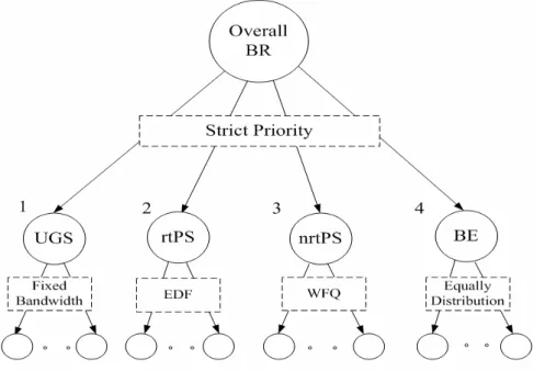
While in the current studies, lots of researches have associated with QoS architecture proposal, the services scheduling of bandwidth allocation is still left with shortage. And some algorithms schedule the traffics simply based on Strict Priority Scheduling [4, 7]. In Strict Priority Scheduling, after BS collects all the bandwidth requests from the connections, it will first classify all them based on the service flow of the connections. Then in each classification, BS uses EDF (earliest deadline first) Queue for the rtPS connections, WFQ (weighted fair) Queue for the nrtPS connections, FCFS (first come first serve) Queue for the BE connections. After the queueing and classification, then schedule them with priority order UGS>rtPS>nrtPS>BE. The allocation method is simply by allocating all the higher priority services bandwidth first, and if there is any spare bandwidth, then allocates lower priority ones. As shown in Fig 1-5.

(22)

Figure 1-5: SPS bandwidth allocation

The advantage of this allocation mechanism is that it can fast attain the QoS guarantees thanks to higher QoS requirement services are first allocated. And the services with short delay requirement can be satisfied. However, if in case the higher priority services overcharge the bandwidth, they may starve the lower priority ones. And the fairness will be seriously affected under this circumstance. While in the definition of [1], the BS needs to urgently allocate in order to satisfy the connections’ Minimum Reserved Rate. After all connections were allocated with their Minimum Reserved Rates, the spare bandwidth should be allocated based on fairness consideration. And the proposed mechanism can also provide QoS guarantees.

1.3 Motivation

Since the services classification based on QoS requirement is defined in the Standard [1], and quite a few researches have proposed the optimal architecture inside BS and SS according to their demand, however the service scheduling is not

(23)

well discussed and proposed in [1] or any other researches. Standard leaves a big room for vendors to implement the detailed operations based on their needs. In the literature so far, only a few documents or researches have been associated with the scheduling algorithm but also lacks of simulation and performance evaluation. In addition, if the scheduling only implements with the strict priority scheduling order (UGS>rtPS>nrtPS>BE), the fairness issue can not be well addressed.

1.3.1 Starvation Problem

That is to say, if in case when bandwidth is not quite sufficient for all the connections and the higher priority services (UGS,rtPS) request for most of the bandwidth, then the lower priority services (nrtPS,BE) would not be able to have chance to get allocated, even if they are allowed to have chance to send Bandwidth Requests. After a period of time, the packets of those connections will expire and then be dropped, finally causing the starvation to happen. In the other case, when sufficient bandwidth is available, but the higher priority connections overcharge bandwidth, resulting in lower priority connections can only be allocated the remaining little bandwidth. And on the other hand, if there is really a very greedy connection who requests almost all the bandwidth, the whole network will probably collapse.

1.3.2 Conservative Bandwidth Allocation Scheduling

There is a way to prevent the starvation problem caused by higher priorities. That is to restrict each connection can only receive at most the size of its Maximum Sustained Rate mapping to one frame (bits/frame). And the allocation order is still with the priority order. It can certainly solve the problem of greedy connections starving lower priority ones. But if the bandwidth is utterly large and only a few

(24)

services have requested bandwidth in the network, a big amount of bandwidth will be wasted because the demanding connections can only be allowed with their maximum sustained rate. To this kind of problem, [6] proposes that bandwidth allocation in a frame can be many rounds. After one round, when there is still available bandwidth, even if all the connections have already been allocated max sustained rate, they can gain the spare bandwidth in the next round. Although this way improves fairness, complicated calculation may become another considerable overhead. Besides, when available bandwidth is not as large as the sum of all connections’ Maximum Sustained Rates, it makes just the same as the priority order scheduling method.

1.3.3 Trustful Bandwidth Allocation Scheduling

Comparing the conservative method that restricts connections are allowed to get a specific number of bandwidth in one frame, we think that trusts the connection by allocating all the bandwidth it needs when it gets the priority is an adaptive way for real network. Once the connection becomes greedy and overcharge causes damages to others connections, a punishment will be brought out. A new priority function will be proposed in the algorithm. Similar with the strict priority defined that the order be (UGS>rtPS>nrtPS>BE), the proposed method can still support the QoS requirement of the different services. Since every connection requests its bandwidth than the BS designs the MAP for next UL- frame, the proposed mechanism discusses only about the uplink transmission based on the fixed size of uplink bandwidth scheme. And the algorithm is a connection based scheduling implemented in BS. Since UGS needs bandwidth in constant size in a constant time, the proposed algorithm does no adaptation to UGS. The scheduling of rtPS, nrtPS, and BE, is after all UGS being allocated.

(25)

1.4 Thesis Organization

In this thesis, the main scope is to expatiate on bandwidth allocation concept of WiMAX. While several papers implemented which so called strict priority queue to address bandwidth in order, but in some cases, the unfair situation may appear. That is why several proceeding researches have another different view of bandwidth allocation. It also proposes a new mechanism of uplink scheduling, which is called two-tier scheduling algorithm, to enhance the shortage of those recent scheduling researches. Under this mechanism, BS (Base Station) can allocate fair bandwidth for each service according to its individual needs. And the fairness concept is obeyed with weighted fairness definition. After the instruction of concept, the simulation result can reveal that the proposed method surely improves performance and guarantees the fairness with quality of service features. The thesis is organized as follows. The second part is the instruction of the two-tier scheduling algorithm and the simulation result will be shown in part three. In the final is the conclusion of the thesis and discuss about the future work of WiMAX.

(26)

Chapter 2. Two-Tier Scheduling Algorithm

2.1 Proposed Structure

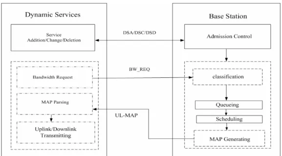
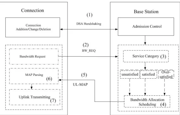
As Fig.5 shows, the service flow handshakes with BS by DSA/DSC message during connection establishing. At this time, this connection will notify BS the two rates as parameters of its own, Maximum Sustained Rate and Minimum Reserved Rate. Once the connection has data to send, it will notify the amount of data to BS by BR. After BS collects all the BRs from connections, it classifies each connection into three category, the first one is the Unsatisfied category, which is for those connections which are not yet satisfied with their minimum guarantee, the second is called Satisfied category, which is for those already satisfied with their minimum guarantee and not yet achieved their maximum requirement, the last category is called Over-satisfied, which is for those already exceed their maximum requirements. BS then performs Queueing and Scheduling operation for them. BS designs the MAP and defines in what time slots which connection can do uplink transmission. Assuming the transmission rate of PHY is fixed, the amount of physical slots mapping to the bandwidth request can be known. Three important parameters will not change by time. And BS can always be aware of each connection’s transmission rate just by the information of elapsed time and allocated bandwidth. The concept of the proposed structure is illustrated in Fig. 2-1.

(27)

Figure 2-1: Proposed structure

2.2 Parameter Definitions

(1) i :

min

R

The Minimum Reserved Rate of connection i. (2) i :

max

R

The Maximum Sustained Rate of connection i.

(3) i :

allocated

R

The previous allocated bandwidth rate of connection i.. (4)PFi:

The Priority Function (PF) of connection i; its value is between [0, 1]. This parameter indicates a connection’s satisfaction degree. Therefore, a connection being with a smaller PF has higher allocation precedence, compared with those

(28)

connections in the same class. The PF in different category has different calculation. And will be shown in 2.4.

2.3 Service Category

(1) Unsatisfied:

In this class, connections are not yet satisfied with their . Thus they are the most urgent ones to get the transmission opportunity. The PF can represent each unsatisfied connection’s satisfied degree. The smaller one shows there is still a long distance to be satisfaction and undoubtedly to be prior allocated. Only rtPS and nrtPS services are qualified in this category because only they two have , while BE has no minimum guarantee. This concept originates from the standard that the key point is to attain each connection’s as soon as possible. As usual, the higher QoS requirement services has larger Minimum Reserved Rate (rtPS>nrtPS), so rtPS services are more possible to be unsatisfied through this measure. As a result, rtPS can usually be prior to be allocated in the next frame than nrtPS even if they were both allocated the same rate in advance.

i min R i min R i min R

(2) Satisfied:

In this category, connections have already been satisfied with their , and so far not reached their . I suggest that after attaining the , the spare bandwidth should be allocated to all the connections through a fair standard. Thus after calculating each connection’s PF, we can know the satisfaction degree of it, i.e., . The connection with lower satisfaction degree should be allocated prior. And those connections which are in a quite satisfied condition should wait until others have been

i min R i max R i min R i PF

(29)

allocated. And at this status, not only rtPS and nrtPS but also BE can take part in the opportunity contention. The can be represented as the max allowable rate contracted with BS. If there is still a long way to this rate, it means this connection is less satisfied. The maximum number of PF is “1”, which stands for the connection is the most satisfied. As usual, the services with higher QoS requirement have larger and . Then after the scheduling of allocation, all connections will be allocated between their . And owing to BE has no , once it is allocated, it will become more satisfied and may become less prior. The result will show that allocated amount in higher QoS requirement services is larger than that in lower ones, which is in accordance with their features. Not only the fairness is guaranteed, but QoS issue has also been concerned.

i max R i max R i min R i min R i min R

(3) Over-satisfied:

In this status, we call those connections as greedy connections. When bandwidth is very sufficient, greedy connections can also be allowed. So after the allocation of Unsatisfied and Satisfied connections, it is time to give chances to those greedy connections. We can still evaluate this kind of connection’s greediness by calculating their . The connections with lower PF stand for less greedy while higher ones are much greedy. Out of fairness, the less greedy connections should be prior to get allocated. As a result, the connection with smaller Maximum Sustained Rate is easier to become greedy and thus less prior to be allocated. Consequently, the lower QoS requirement service, such as Best Effort, is less prior once it is in this category. On the other hand, we also propose a parameter called , the larger

can make to become smaller, thus the higher QoS requirement services can be prior to be allocated than lower ones in this category.

i PF i QoS_Fac QoS_Fac_i i PF

(30)

2.4 Priority Function Calculation

Based on the current service category of connection i, its PF is calculated as follows. i i i allocated allocated min i min i i i i i allocated min

i i i min allocated max max min i i i i allocated max allocated max i i allocated i

R

, if R

<R

R

-R

PF =

, if R

R

-R

R

-R

, if R

>R

QoS_Fac

R

3, if i rtPS

QoS_Fac = 2, if i nrtPS

1, if i BE

⎧

⎪

⎪⎪

_≤

⎨

⎪

×

⎪⎩

∈

⎧

⎪

⎨

⎪

⎩

2.5 Two-Tier Scheduling Operations

Tier 1:

During the connection establishing period, connections do the handshaking with BS and notify the and to BS. Then if a connection has data to send, it will notify the BS by sending BR before BS designing MAP.

i m i n

R i m ax

R

After collecting all the BRs in one frame, BS calculates each connection’s and classifies all the connections into three categories.

i a llo c a te d

R

Tier 2:

When in each frame, the BS allocates bandwidth (BW) following the category order (UnsatisfiedÆSatisfiedÆOver-satisfied). In each category, always pick up the connection with the smallest PF and allocate bandwidth to it according to its BR until all bandwidth is allocated. When finishing all the allocation in one category, if there is

(31)

still available bandwidth, then enter the next category allocation. If all bandwidth is allocated in any category or all connections are allocated after Over-satisfied category, BS stops the process and broadcasts MAP. However, in the initial frame, while all connections’ PFs are zero, and no priority order can be evaluated, the scheduling algorithm simply allocates to connections following first come first serve (FCFS) scheduling. And then in the later frames, the connections with allocated bandwidth have PF values while those not allocated connections have PF value of zero and become prior. The process of Two-Tier Scheduling Algorithm (2TSA) can be illustrated as the pseudo code and in flow chart in Fig. 2-2 shown below.

(32)

Pseudo Code of 2TSA

(33)

Chapter 3. Performance Evaluation

3.1 Parameter and Environment Setting

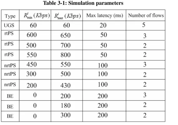
The simulation program is based on a self-configured environment with g++ compiler in Linux, and modified from a part of settings in [6]. Simulation environment is under deploying five connections of UGS flows, seven of rtPS flows, seven of nrtPS flows, and seven of Best Effort flows. For each UGS flow, we define their max latency of 20(ms), both Minimum Reserved Rate and Maximum Sustained Rate of 60Kbits/sec. For each rtPS flows, we define Max latency as 50(ms). For nrtPS flows, we define their Max Latency as 100(ms). And for BE flows, define their Max Latency as 200(ms). Buffer management is used to control buffer and decide which packet to drop. When the waiting time of some packets exceeds their max latency, buffer will regard them as invalid packets and drop. Frame length is assigned to 10 ms and simulation time is 1000 frames (10 seconds). The simulation parameters are illustrated in Table 3-1.

(34)

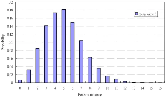
All packet arrivals occur at the beginning of each frame and the packet arrival process for each connection follows the Poisson distribution with different traffic rate λ. We propose that each connection generates at least its Minimum Reserved Rate mapping to one frame. And the average generated size in one frame is designed to its Maximum Sustained Rate mapping to one frame. By defining fixed packet size, we can implement the packet arrival model that follows Poisson Process [10], which illustrates the distribution the number of arrival packets in on frame, and it is defined with

λ λ

, is the mean value of arrival packets numbers. Thus defined:

Table 3-1: Simulation parameters

i i

max min

R -R λ=

(35)

0 0.02 0.04 0.06 0.08 0.1 0.12 0.14 0.16 0.18 0.2 0 1 2 3 4 5 6 7 8 9 10 11 12 13 14 15 16 Poisson instance P roba bilit y mean value 5

Figure 3-1: Poisson distribution

The Fig. 3-1 shows the Poisson distribution with mean ( ) value is five. The simulation model bounds connections’ generated packets in each frame to its Minimum Reserved Rate mapping to one frame, and generates packets variably every frame. Average traffic rate is its maximum sustained rate.

λ

Besides, in the simulation, we also simulated the greedy connections’ behavior. In the first five seconds, connections generate and request bandwidth follows their Maximum Sustained Rate. However after simulation time of five seconds, if any connection finds out that its allocation is in a good condition. It will attempt to request more bandwidth for better throughput. In that case, connection is becoming greedy because its average Bandwidth Request is enlarging. And as also, after another period of time, if the greedy connection detects that the condition is still good, it will request more. Observation is about to see the fairness improvement when some connections become greedy and intend to cause damages to other connections.

The simulation runs under two available bandwidth scenarios. The performance of Two-Tier Scheduling Algorithm(2TSA) and Strict Priority Scheduling(SPS) will be

(36)

compared. First, set the available bandwidth between the summation of all connections’ Maximum Sustained Rates and Minimum Reserved Rates. As the performance expected, all the connections should be in the category of Satisfied after simulation by the proposed mechanism. And compare with the SPS method that allows greedy rtPS starve nrtPS and BE. In the second scenario, set the available bandwidth to be larger than the summation of total connections’ Maximum Sustained Rates. In Scenario II, two cases will be run. One is by assuming only rtPS becomes greedy after five seconds and the other is by assuming all connections are able to become greedy. Observation in the first case is about to see if overcharging rtPS will starve nrtPS or BE. The second case is about to see whether the allocation of residual bandwidth is more fairly allocate to all connections and also benefit the higher QoS requirement connections to take more than the lower ones

3.2 Performance Metrics

The performance metrics measured in the simulation include the average throughput and fairness degree.

(1) Average throughput(Φ )_j

This parameter is defined as the average allocated bandwidth. As the following equation shows, for class j, and connection i,

∑

B i i j j j andwidth_usage Φ = n ∈

Where Bandwidth usage_ _i is the allocated bandwidth of connection i, and

n

j is

(37)

(2) Fairness degree (FD):

This parameter indicates how fair the bandwidth is shared by all connections for each approach, and is defined as:

( )

2 1 2 1 FD n i n i SD i n SD i = = ⎡ ⎤ ⎢ ⎥ ⎣ = ⎡ ⎤ ⎣ ⎦

∑

⎦ _{, where n is the number of connections and Share degree (SD)}

defines as:

( )

min max min

SD

i i allocated i i

R

i

R

−

=

−

, SD indicates the relation between a connection’s demand

and allocated bandwidth. The FD value is between [0,1]. It represents the variant between connections’ SDs. The smaller the variant is, the larger FD will be, and the allocation will be fairer.

(3) Average delay:

This parameter indicates the average delay of each class of service type. The value is calculated in milliseconds (ms). We calculated this metric based on the packets sent and the total delay of sent packets. In case the flow gets starvation, the average delay after starvation will be regarded as zero.

(4) Throughput per connection:

We have also reckoned up each connection’s throughput in the final of simulation. This value was calculated based on each connection’s actual allocated bandwidth during simulation and the simulation time. Besides, the result will be shown in Table format.

(38)

3.3.1 Scenario I: Available bandwidth 8Mbits/sec

In the first scenario, the available bandwidth is set to 8 Mbits/sec. When using strictly priority scheduling, only rtPS can be allocated with its Maximum Sustained Rate. Although allocating bandwidth to rtPS and UGS connections, the residual

bandwidth is, (Mbits) , it is not enough

for all nrtPS with their Maximum Sustained Rate ,i.e., .Of course, BE connections starved. As Fig 3-2 shows, in the beginning five seconds, rtPS connections are allocated with Maximum Sustained Rate, while nrtPS were allocated less than this rate, and BE could not gain any bandwidth. In the later five seconds, some rtPS became greedy and attempted to grab nrtPS’s bandwidth. As a result, nrtPS will be allocated even less than their Minimum Reserved Rate. The fairness index shown in Fig 3-3 also indicates this damage of fairness. In the first five seconds, the fairness degree converges around 0.2~0.3 owing to the no allocation to BE. However, the stable state of fairness degree was broken and seriously decreased when the greedy connections appeared in the later five seconds. On the other hand, when using 2TSA, all connections share bandwidth proportionally, and none exceeds the Maximum Sustained Rate. In Fig 3-3, the fairness degree remains almost one, even when some connections become greedy. The reason is that once a connection gets more bandwidth in current frame, it will lose its priority in the following frames. Thus, even when rtPS became greedy in the last five seconds, they were only able to get the same rate as before. We can see at the beginning, the fairness degree does not sustain one but in the following seconds, the fairness degree almost performs one. However on the contrary, the throughput performs the same from start to the end. That is because we evaluate throughput every interval by interval. And while calculating fairness

8 (0.06 5) (0.65 3 0.8 2 0.7 2) 2.75− × − × + × + × =

(39)

0 200 400 600 800 1000 1200 1 2 3 4 5 6 7 8 9 10 Simulation time(sec) Thr oug hp ut (K bi ts /s ec) 2TSA-rtPS 2TSA-nrtPS 2TSA-BE SPS-rtPS SPS-nrtPS SPS-BE

Figure 3-2: Average throughput in Scenario I

0 0.2 0.4 0.6 0.8 1 1.2 1 2 3 4 5 6 7 8 9 10 Simulation time(sec) Fa irne ss de gree 2TSA SPS

Figure 3-3: Fairness degree in Scenario I

degree, we used the globally allocated bandwidth for index.

In the average delay of Scenario I, we can see that in SPS. rtPS < nrtPS, and BE is zero due to its starvation. rtPS remains in a very short delay because SPS supports its QoS priority. However, if we continue to see the 2TSA performance, rtPS remains

(40)

average delay of 20ms and nrtPS performs shorter delay than that in SPS. On the other hand, owing to the non-starvation of BE. BE also performs average delay about 120 ms. The simulation figure is shown below Fig.3-4. All connection’s throughputs are shown in Table. 3-2, 3-3, and 3-4.

0 20 40 60 80 100 120 140 1 2 3 4 5 6 7 8 9 10 Simulation time(sec) Ave rage delay( m s) 2TSA-rtPS 2TSA-nrtPS 2TSA-BE SPS-rtPS SPS-nrtPS SPS-BE

Figure 3-4: Average delay in Scenario I

(41)

Table 3-3: Throughput of nrtPS in 2TSA Scenario I

(42)

3.3.2 Scenario II: Available bandwidth 12Mbits/sec

In the second scenario, the available bandwidth is set to 12 Mbits/sec. And two cases are simulated in this scenario. One is by assuming only rtPS connections become greedy after five seconds and the other one is by assuming all connections are able to become greedy after five seconds as long as they find out their previous allocation quality is good and try to send more data in purpose of better throughput. When using Strict Priority Scheduling, the three types of services were originally allocated with their Maximum Sustained Rate, Fig.3-5, Fig.3-6, because the available bandwidth (12Mbits) is larger than the summation of all the connections’ Maximum Sustained Rates. And the remaining bandwidth becomes residual bandwidth.

(12 ), in the first five

seconds, the stable state of fairness degree has been remained, Fig. 3-7. But in the later five seconds, rtPS started grabbing bandwidth and made nrtPS and rtPS seriously damaged. Sooner or later, the nrtPS and BE will be starved. In Fig.3-7, the fairness degree downs to almost zero at the end, which means it is a very unfair state. No matter in which case, starvation of nrtPS and BE will happen. However, if using 2TSA, in the first five seconds, each service gained their Maximum Sustained Rate. And in this scenario, the spare bandwidth (12-10.32=1.68Mbits) is not used and become residual bandwidth. When simulation time went over five seconds, in Case 1, see Fig.3-5, the rtPS connections attempted to gain the residual bandwidth and successfully be allocated. But the difference between Strict Priority Scheduling is that, when rtPS overcharges, nrtPS and BE will not be damaged. And in Case 2, see Fig.3-6, because all the connections are able to become greedy, the residual bandwidth will be fairly allocated to the connections which request more. The residual allocation of each connection is also different based on its QoS requirement.

0.3(UGS) 4.95(rtPS) 3.51(nrtPS) 1.56(BE) 10.32Mbits

(43)

And it is resulted from the design of QoS_Fac, connections with higher QoS requirement are assigned with a higher QoS_Fac and generated a lower PF. As a result, we can see the residual bandwidth allocation is rtPS>nrtPS>BE. Then in the evaluation of the fairness degree in Fig 3-6, when after five seconds, fairness will surely be affected by the rtPS in Case 1 either SPS or 2TSA. But the damage of fairness in 2TSA is obviously much less than that in SPS. If in Case 2, owing to all the connections will be able to become greedy after five seconds, the fairness degree of 2TSA outperforms the Case 1 in 2TSA. No matter which case we run. The fairness degree of SPS decreases seriously once rtPS connections starve nrtPS and BE ones. And in Fig 3-8 is the long term(100 seconds) of observation. Even the fairness degree of 2TSA decreases in the first few seconds, it will converge at the end and again remain a stable state.

(44)

Figure 3-5: Average throughput in Scenario II-Case 1

(45)

0 0.2 0.4 0.6 0.8 1 1.2 1 2 3 4 5 6 7 8 9 10 Simulation time(sec) Fa ir ne ss de gr ee 2TSA-case 1 2TSA-case 2 SPS-case 1 SPS-case 2

Figure 3-7: Fairness degree in Scenario II-10 seconds

0 0.1 0.2 0.3 0.4 0.5 0.6 0.7 0.8 0.9 1 10 20 30 40 50 60 70 80 90 100 Simulation time(sec) F ai rn es s degr ee 2TSA-case 1 2TSA-case 2 SPS-case 1 SPS-case 2

Figure 3-8: Fairness degree in Scenario II-100 seconds

The average delays of Scenario II are shown in Fig. 3-9 and Fig. 3-10. In case 1, only rtPS become greedy, and rtPS lengthens its average delay after five seconds

(46)

owing to some of the rtPS may also be affected by other greedy rtPS, no matter in SPS or 2TSA. The connections of nrtPS and BE in SPS remain the same after five seconds owing to all the bandwidth are deprived by rtPS and became starved. Thus, no more packets can be sent after five seconds in nrtPS or BE. On the other hand, though rtPS performs longer delay in 2TSA than in SPS, the nrtPS and BE performs shorter delay in 2TSA than those in SPS, which is also following our fairness prediction. In the second case of the scenario, all services performed longer delay in 2TSA after five seconds. This is because everyone is greedy and generated more. However, the fairness mechanism manages no one can deprive others bandwidth. In consequence, some of the generated packets have to wait for longer time. In both scenario and the two cases in scenario II, average delay is rtPS< nrtPS < BE. This outcome shows 2TSA supports QoS requirement in delay issue. At the end, Table.3-5, 3-6, and 3-7 show the throughput of each connection.

(47)

0 2 4 6 8 10 12 1 2 3 4 5 6 7 8 9 10 Simulation time(sec) Average delay( ms) 2TSA-rtPS 2TSA-nrtPS 2TSA-BE SPS-rtPS SPS-nrtPS SPS-BE

Figure 3-9: Average delay in Scenario II- case 1

0 5 10 15 20 25 30 35 40 1 2 3 4 5 6 7 8 9 10 Simulation time(sec) Average delay(ms) 2TSA-rtPS 2TSA-nrtPS 2TSA-BE SPS-rtPS SPS-nrtPS SPS-BE

(48)

Table 3-5: Throughput of rtPS in 2TSA Scenario II

Table 3-6: Throughput of ntPS in 2TSA Scenario II

(49)

Chapter 4. Conclusion & Future Work

In this thesis, first a brief introduction of WiMAX was made. Then an overview of WiMAX was presented. WiMAX is defined as IEEE 802.16 and is also named as Broadband Wireless Network. And the scope discussed here is focused on Uplink Service Scheduling in TDD transmission mode. The three important parameters play important roles in service management. Then we brought out a new proposed structure illustrating the interaction between connections and BS with explaining why to make the services classified into three. The Unsatisfied category, the Satisfied category, and the Over-satisfied category. Then this thesis proposed a new uplink scheduling algorithm based on the computation from Minimum Reserved Rate and Maximum Sustained Rate. After that, the evaluation the fairness degree by a fairness index was designed. Through some different settings of simulation, results show that the proposed algorithm really outperforms the Strictly Priority Scheduling in the fairness issue. And in addition to efficiently prevent starvation, this proposed algorithm can also manage the greedy connections.

In the future work, we will investigate bandwidth allocation considering other QoS metrics, such as delay or delay jitter, for WiMax networks. Though we made no adaptation relating to the Max Latency, the delay issue may be another critical point. When in the high QoS requirement services, such as real time video, the generated size is not constant. And maybe in some times, very urgent and large data need to be sent. So how to reduce the delay and at the same time guarantees the fairness is another goal needs to be achieved.

(50)

Reference

[1] IEEE 802.16 Standard-Local and Metropolitan Area Networks-Part 16. IEEE 802.16-2004

[2] Dong-Hoon Cho, Jung-Hoon Song, Min-Su Kim, and Ki-Jun Han, “Performance Analysis of the IEEE 802.16 Wireless Metropolitan Area Network”, Distributed

Frameworks for Multimedia Applications, 2005. DFMA '05. First International Conference, Page(s):130 – 136, Feb. 2005

[3] Hamed S. Alavi, Mona Mojdeh, Nasser Yazdani, “A Quality of Service Architecture for IEEE 802.16 Standards”, 2005 Asia-Pacific Conference on

Communications, Perth, Western Australia, Page(s):249 – 253, 03-05 Oct. 2005

[4] Kitti Wongthavarawat, Aura Ganz, “IEEE 802.16 BASED LAST MILE BROADBAND WIRELESS MILITARY NETWORKS WITH QUALITY OF SERVICE SUPPORT”, Military Communications Conference, 2003. MILCOM 2003.

IEEE, Page(s):779 - 784 Vol.2, 13-16 Oct. 2003

[5] Qingwen Liu, Xin Wang and Georgios B. Giannakis, “Cross-Layer Scheduler Design with QoS Support for Wireless Access Networks”, Quality of Service in

Heterogeneous Wired/Wireless Networks, 2005. Second International Conference,

Aug. 2005.

[6] Jianfeng Chen, Wenhua Jiao, Hongxi Wang, “A Service Flow Management Strategy for IEEE 802.16 Broadband Wireless Access Systems in TDD Mode”,

Communications, 2005. ICC 2005. 2005 IEEE International Conferenc,

Page(s):3422- 3426, May 2005.

[7] Hawa, M.; Petr, D.W.,”Quality of service scheduling in cable and

broadband wireless access systems”, Tenth IEEE International Workshop on Quality

(51)

[8] K. Wongthavarawat, and A. Ganz, “Packet Scheduling for QoS Support in IEEE 802.16 Broadband Wireless Access Systems”, International Journal of

Communication Systems, Vol. 16, p81-96, 2003

[9] Spyros A, Xergias Nikos Passas, and Lazaros Merakos, “Flexible Resource Allocation in IEEE 802.16 Wireless Metropolitan Area Networks”, Local and

Metropolitan Area Networks, 2005. LANMAN 2005. The 14th IEEE Workshop, Sep

WiMAX網路上傳具品質服務保證之公平排程機制

國

立

交

通

大

學

資訊科學與工程研究所

碩

士

論

文

WiMAX 網路上傳具品質服務保證之公平排程

機制

Fair Scheduling with QoS Guarantees for Uplink

Transmission in WiMAX Network

研 究 生：詹林峰

指導教授：趙禧綠 助理教授

Abstract

摘要

致謝

Contents

List of Figures

List of Tables

Chapter 1. Introduction

1.1 WiMAX Background Overview

1.1.1 Frame

Structure

UL Subframe

DL Subframe

Frame j

Frame j-1

Frame j-2

Frame j+1

Frame j+2

1.1.2 Connection

Identifier

1.1.3 Service Flow Creation

1.1.4 Bandwidth

Request

Message

1.1.5 Service

Flows

Management

1.1.5.1 Minimum Reserved Rate

1.1.5.2 Maximum Sustained Rate

1.1.5.3 Max Latency

1.1.6 Different Service Types Defined in WiMAX

1.1.6.1 Unsolicited Grant Service (UGS)

1.1.6.2 Real Time Polling Services (rtPS)

1.1.6.3 Non Real Time Polling Service (nrtPS)

1.1.6.4 Best Effort Services (BE)

1.2

Related Work

1.3

Motivation

1.3.1 Starvation Problem

1.3.2 Conservative Bandwidth Allocation Scheduling

1.3.3 Trustful Bandwidth Allocation Scheduling

1.4 Thesis Organization

Chapter 2.

Two-Tier Scheduling Algorithm

2.1 Proposed Structure

2.2 Parameter Definitions

2.3 Service Category

(1) Unsatisfied:

(2) Satisfied:

(3) Over-satisfied:

2.4 Priority Function Calculation

R

, if R

<R

R

R

-R

PF =

, if R

R

R

R

研究生：詹林峰

指導教授：趙禧綠助理教授

_≤

_≤