國
立
交
通
大
學
應用數學系
碩
士
論
文
三角形棒棒糖圖的無號拉普拉斯矩陣之特徵值探討
Signless laplacian spectrum of a lollipop graph with a triangle
研
究 生:徐志杰
指導教授:翁志文
教授
三角形棒棒糖圖的無號拉普拉斯矩陣之特徵值探討
Signless laplacian spectrum of a lollipop graph with a triangle
研 究 生:徐志杰
Student:
Chih-chieh Hsu指導教授:翁志文
Advisor:
Chih-wen Weng國 立 交 通 大 學
應 用 數 學 系
碩 士 論 文
A Thesis
Submitted to Department of Applied Mathematics College of Science
National Chiao Tung University in partial Fulfillment of the Requirements
for the Degree of Master
in
Applied Mathematics June 2013
Hsinchu, Taiwan, Republic of China
三角形棒棒糖圖的無號拉普拉斯矩陣之特徵值探討
研究生:徐志杰 指導老師:翁志文 教授
國 立 交 通 大 學
應 用 數 學 系
摘 要
假設 G 是一個由點 1 2 … n 所構成的簡單圖,其中每個點相對應的價數 分別為 d1 d2 … dn 設 A(G) 是 G 的 (0,1)-鄰接矩陣,D(G) 是一個對角 矩陣,其對角線上分別是 d1 d2 … dn 矩陣 L(G)=D(G)-A(G) 稱為 G 的 拉普拉斯矩陣,矩陣 |L|(G)=D(G)+A(G) 稱為 G 的無號拉普拉斯矩陣 A(G),L(G),|L|(G) 的特徵值給了我們很多訊息去了解 G 的構造 在這個論 文中,我們研究一種圖形叫做三角形棒棒糖圖,其由一個三個點的完全圖與 一個路徑圖共用一點而接起來 我們探討三角形棒棒糖圖的無號拉普拉斯矩 陣的特徵值 特徵多項式及它們的相關比較問題 關鍵詞:棒棒糖圖 無號拉普拉斯矩陣 特徵值 iSignless laplacian spectrum of a lollipop graph
with a triangle
Student: Chih-chieh Hsu
Advisor: Chih-wen Weng
Department o f Applied Mathematics National Chiao Tung U niversity
Abstract
Let G be a simple graph with vertices 1,··· ,n of degrees d1,··· ,dn respectively. Let
A(G) be the (0, 1)-adjacency matrix of G, and let D(G) be the diagonal matrix diag(d1,··· ,dn). The matrix L(G) = D(G)−A(G) is the Laplacian matrix of G, while |L|(G) = D(G)+A(G) is called the signless laplacian matrix of G. The eigenvalues of A(G), L(G), and|L|(G) give many hints to the structure of G. In this thesis we study a class of graphs, called lollipop graph with a triangle, which are obtained from paths by adding a new vertex to a path and adding two edges from the new vertex to one end of the path and to the neighbor of this end, forming a triangle K3. We study the signless Laplacian eigenvalues and characteristic
polynomial of lollipop graphs with K3.
誌
謝
來到交大已經兩年了,這兩年有許多美好的回憶,也很幸運的能夠準
時完成學業,這一路上要感謝很多人 其中最感謝的是我的指導教授
翁志文,沒有老師的耐心,是沒辦法完成這篇論文的,真的很感謝老
師這兩年來的幫助
再來要謝謝康明軒老師 傅恆霖老師 符麥克老師,每一位老師的課
程都讓我收穫豐富,感謝陳秋媛老師常來我們研究室關心我們的近況,
還有舉辦很多很棒的活動,感謝同門的王秉鈞在生活上的幫忙,在研
究上的幫助,感謝李光祥學長對我論文上的建議以及幫助,劉家安學
長抽空陪我們模擬口試,也要感謝王紹鈞 林立庭等組合學的同學們,
跟你們一起真的很開心,讓我留下了美好的回憶,也是我一生中一段
蠻值得回憶的時光
感謝我的父母親以及阿嬤,每次回家都這麼的關心我,給我這麼多關
懷以及支持,讓我在求學之路上可以毫無顧忌,感謝我的女友,沒有
妳我是沒辦法在這裡打這篇誌謝的
要感謝的人太多了,人生無不散的宴席,能留下的只有心中的回憶
iiiContents
Abstract (in Chinese) i
Abstract (in English) ii
Acknowledgements iii Contents iv 1 Introduction 1 2 Preliminaries 2 2.1 Graphs . . . 2 2.2 Matrices . . . 3 2.3 Characteristic polynomial . . . 4
2.4 Interlacing of two sequences . . . 5
3 Basic properties 5 3.1 Rayleigh’s principle . . . 5
3.2 Interlacing property for edge deleting . . . 7
3.3 Bounds of the largest signless laplacian eigenvalue . . . 10
4 Main Results 10 4.1 The least eigenvalue of L3,2 . . . 11
1
Introduction
Let G be a simple graph with vertices 1,··· ,n of degrees d1,··· ,dnrespectively. Let A(G) be the
(0, 1)-adjacency matrix of G, and let D(G) be the diagonal matrix diag(d1,··· ,dn). The matrix
L(G) = D(G)− A(G) is the Laplacian matrix of G, while |L|(G) = D(G) + A(G) is called the
signless laplacian matrix of G. The eigenvalues of A(G), L(G), and|L|(G) give many hints to the structure of G. The least eigenvalue of L(G) is always zero, and the second least is known as the algebraic connectivity of G, which is related to the connectivity of G in some sense[1]. It is well-known that the numbers of distinct eigenvalues of A, L(A), and|L|(G) respectively are at least one plus the diameter of G[4].
A bipartite graph is a graph whose vertices can be divided into two disjoint sets U and V such that every edge connects a vertex in U to one in V; that is, U and V are each independent sets[2, 3]. For the case that G is bipartite, the eigenvalue of L(G) are that of|L|(G). We are interested in the determination of eigenvalue of|L|(G) for a non-bipartite graph G.
The simplest connected graphs which are not bipartite are trees with one more edge. If we add an edge to a tree to make a graph G with an odd-length cycle, then the least eigenvalue of|L|(G) is not zero. Besides this, to let G have the longest diameter, we study the graph G which is obtained from a path by adding one more vertex with two neighbors: one end of the path and the neighbor of this end. The graph G is called a lollipop graph with K3of order n,
denote by L3,n−3. The paper [5] tells us that signless Laplacian matrix of a lollipop graph with
K3has the least Laplacian eigenvalue among all non-bipartite connected graphs of order n. We
eigenvalues of|L|(L3,n−3).
Thesis is organized as following. First we give some definitions in graph theory and matrix theory in Section 2. In Section 3, some propositions which will be used in the thesis are given. Our main results are given in Section 4. By using a simple example, we introduce a method to compare the least Laplacian eigenvalues of two graphs with the same number of edges. We study the upper bound of the largest Laplacian eigenvalues of lollipop graphs with K3 by
using known results and using computer software Mathematica. We compute the characteristic polynomial Pn(λ) of|L|(L3,n−3) and find a three-term recurrence relation of Pn(λ). Then we
find 1 is a common eigenvalue of L3,n−3 and determine its multiplicity.
2
Preliminaries
In this section, we introduce notations which we will use in this thesis.
2.1
Graphs
A graph G considered in the thesis is finite, undirected, and connected, without loops or multiple edges. We use V (G) to denote the vertex set and E(G) to denote the edge set of G, usually
V (G) = [n] ={1,2,...,n}. The cardinality |V(G)| is called the order of G. The following
special graphs with vertex set [n] and their corresponding symbols are used in the thesis.
1. The complete graph Kn: E(Kn) ={i j | 1 ≤ i < j ≤ n}.
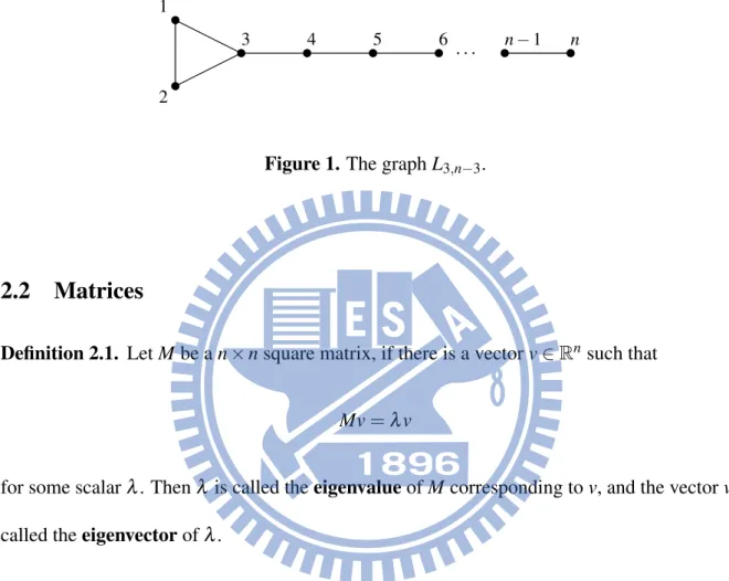
3. The (m, n− m)-lollipop Lm,n−m: E(Lm,n−m) ={i j | 1 ≤ i < j ≤ m} ∪ {i i + 1 | m ≤ i ≤
n− 1}, where m ≤ n. See Figure 1 for L3,n−3.
t 1 t 2 t 3 t4 t5 t6 tn− 1 tn ···
Figure 1. The graph L3,n−3.
2.2
Matrices
Definition 2.1. Let M be a n× n square matrix, if there is a vector v ∈ Rnsuch that
Mv =λv
for some scalarλ. Thenλ is called the eigenvalue of M corresponding to v, and the vector v is called the eigenvector ofλ.
Let G be a graph of order n. The matrices considered in the thesis are all symmetric over the real number fieldR whose rows and columns are indexed by V(G). Let D(G) denote the diagonal matrix with rows and columns indexed by vertices of G such that D(G)xx= d(x) which
the d(x) is degree of x in G. Then the adjacency matrix A(G), Laplace matrix L(G), signless laplacian matrix|L|(G) are defined as follows.
(i) A(G)xy= 1, if xy∈ E(G); 0, otherwise.
(ii) L(G) = D(G)− A(G),
(iii) |L|(G) = D(G) + A(G).
In the thesis, we only study the signless lpalacian matrix|L|(G) of a graph G.
Let q1(G)≥ q2(G)≥ ··· ≥ qn(G) be the eigenvalues of|L|(G), and we refer to this sequence
as the spectrum of|L|(G), or that of G for short. If the graph G is clear, we might delete the symbol G in a notation ℓ(G) and write it as ℓ.
We use the symbol G\ e to denote the graph with the same vertex set as V(G) and obtained by deleting the edge e of G.
2.3
Characteristic polynomial
The characteristic polynomial of a square matrix M is the polynomial det(λI−M). It is
well-known that the eigenvalues of M are the roots of the characteristic polynomial of M.
The following example will be uesed in Lemma 4.1 and 4.6
Example 2.2. |L|(L3,1) = 2 1 1 0 1 2 1 0 1 1 3 1 0 0 1 1 ,|L|(L3,2) = 2 1 1 0 0 1 2 1 0 0 1 1 3 1 0 0 0 1 2 1 0 0 0 1 1 .
Then det(λI− |L|(L3,1)) = λ4− 8λ3+ 19λ2− 16λ+ 4, det(λI− |L|(L3,2)) = λ5− 10λ4+ 34λ3− 48λ2+ 27λ− 4. The spectrum of|L|(L3,1) is{5− √ 17 2 , 1, 2, 5+√17
2 }, and the spectrum of |L|(L3,2) is
{0.2243,1,1.4108,2.7237,4.6412}, computed by Mathematica.
2.4
Interlacing of two sequences
For m < n, a sequenceλ1≥λ2≥ ··· ≥λmof real numbers is said to interlace another sequence
q1≥ q2≥ ··· ≥ qnof real numbers if
qi≥λi≥ qn−m+i for 1≤ i ≤ m.
3
Basic properties
In this section, we shall review a few basic properties in matrix theory and some previous results in the study of spectrum of a graph. For completeness, we shall provide the proofs of some properties.
3.1
Rayleigh’s principle
It is well-known that the largest eigenvalueλ1and the least eigenvalueλnof a symmetric matrix
M or order n satisfy λ1= max 0̸=x∈Rn x⊤Mx x⊤x , λn= min0̸=x∈Rn x⊤Mx x⊤x .
The following proposition generalizes this property.
Proposition 3.1. Let M be a real symmetric matrix of order n with eigenvaluesλ1≥λ2≥ ··· ≥
λnand respective orthonormal eigenvectors u1, u2,··· ,un. Then
(i) u
⊤Mu
u⊤u ≥λifor any u∈ Span(u1, u2,··· ,ui), and equality holds iff u is an eigenvector of M corresponding toλi,
(ii) u
⊤Mu
u⊤u ≤λi+1for any u∈ Span(u1, u2,··· ,ui)
⊥, and equality holds iff u is an eigenvector
of M corresponding toλi+1.
Proof. (i) Write u = c1u1+··· + ciuifor some cj∈ R, j = 1,2,··· ,i. Then
u⊤Mu
u⊤u =
c21λ1+ c22λ2+··· + c2iλi
c21+ c22+··· + c2i ≥λi.
If u is an eigenvector of M corresponding toλi, then by the definition of eigenvector,
Mu = λiu,
u⊥Mu = u⊥λiu,
u⊥Mu = λiu⊥u,
u⊥Mu
u⊥u = λi.
Hence the equality holds. If the equality holds, thenλj=λiif cj̸= 0, where j ≤ i. Hence
u is an eigenvector of M corresponding toλi.
(ii) Similar to the above proof except here we use
3.2
Interlacing property for edge deleting
We shall show that deleting an edge from a graph G does not increase any value of the spectrum of G.
Definition 3.2. An m×m matrix P is a principal submatrix of an n×n matrix M, where m < n, if P is obtained from M by removing any n− m rows and the same n − m columns.
The following lemma describes the relation between eigenvalues of a symmetric matrix and that of its principal submatrix.
Lemma 3.3. If an m× m matrix P is a principal submatrix of an n × n symmetric matrix M,
where m < n, then the eigenvalues of P interlace those of M.
Proof. To simplify the notation, we may assume P is obtained from M by removing the last n−m rows and columns. Then we can write P = S⊤MS, where S is an n×m matrix of the form
Im 0(n−m)×m , and Imis the m× m identity matrix. In particular S⊤S = Im.
Let u1, u2,··· ,un be orthonormal eigenvectors of M corresponding to eigenvalues λ1 ≥
λ2≥ ··· ≥λnrespectively and v1, v2,··· ,vmbe orthonormal eigenvectors of P corresponding to
eigenvaluesη1≥η2≥ ··· ≥ηmrespectively. Note that
dim (
Span(v1, v2,··· ,vi)∩ Span(S⊤u1, S⊤u2,··· ,S⊤ui−1)⊥
)
≥ i + (n − i + 1) − n = 1.
Hence there exists a nonzero vector si∈ Span(v1, v2,··· ,vi)∩ Span(S⊤u1, S⊤u2,··· ,S⊤ui−1)⊥.
Rayleigh’s principle, λi≥ (Ssi)⊤M(Ssi) (Ssi)⊤(Ssi) = (si) ⊤P(s i) (si)⊤(si) ≥η i.
By applying the above inequality to−M and −P we getλn−m+i≤ηi. Hence
λn−m+i≤ηi≤λi.
Definition 3.4. Let M denote the (vertex-edge) incidence matrix of G, i.e. M is a matrix with rows indexed by vertices and columns indexed by edges, such that for x∈ V(G) and e ∈ E(G),
Mxe= 1, x∈ e; 0, otherwise.
The following lemma describes the relation between incidence matrix and signless lpalacian matrix.
Lemma 3.5. Let M be the incidence matrix of G. Then|L|(G) = MM⊤. Proof. Note that for x, y∈ V(G),
(MM⊤)xy=
∑
e Mxe(M⊤)ey= 1, if xy∈ E(G); d(x), if x = y; 0, otherwise, = (|L|(G))xy,where d(x) is the degree of x.
The following lemma indicates the relation between two matrices which have the same eigenvalues.
Lemma 3.6. Let N be an n× m matrix. Then there exists a one-one correspondence between
the nonzero eigenvalues of NN⊤ and N⊤N.
Proof. Suppose q is a nonzero eigenvalue of NN⊤ with corresponding eigenvector u. Then
NN⊤u = qu̸= 0. In particular N⊤u̸= 0. Since N⊤NN⊤u = qN⊤u, N⊤u is an eigenvector of N⊤N corresponding to the eigenvalue q. Suppose q has multiplicity m as an eigenvalue of NN⊤.
Let u1, u2,··· ,umbe the corresponding orthogonal eigenvectors. If c1N⊤u1+···+cmN⊤um= 0
then
0 = N(c1N⊤u1+··· + cmN⊤um) = q(c1u1+··· + cmum),
and hence c1= c2=··· = cm= 0. This proves that the multiplicity of q in NN⊤ is no larger
than that in N⊤N. Similarly for the other side, so the two multiplicities are the same.
The following proposition demonstrates the interlacing property for edge deleting.
Proposition 3.7.
qi+1(G)≤ qi(G\ e) ≤ qi(G) for 1≤ i ≤ n − 1.
Proof. Let M denote the vertex-edge incidence matrix of G and recall that|L|(G) = MM⊤ by Lemma 3.5. Note that the incidence matrix M′of G\ e is obtained from M be deleting the col-umn associated with e. Hence M′⊤M′is a principal submatrix of M⊤M. By interlacing property
in Lemma 3.3, the sequence of eigenvalues of (n−1)×(n −1) matrix M′⊤M′interlaces that of
n× n matrix M⊤M. Since M⊤M and MM⊤ have same nonzero eigenvalues by Lemma 3.6, we
have
3.3
Bounds of the largest signless laplacian eigenvalue
We shall provide some known bounds of the largest eigenvalue q1(G) of G. For v ∈ V(G),
denote the neighbor of v by N(v), and define
m(v) :=
∑
u∈N(v)
d(u) d(v),
the average of the degrees of the vertices adjacent to v. Let∆(G) be the maximal degree of G and Nibe the set of the neighbor of the vertex vi. The following proposition is well-known.
Proposition 3.8. [6]
(i) q1(G)≤ max{d(vi) + d(vj) : vivj∈ E(G)},
(ii) q1(G)≤ max{m(vi) + d(vi) : vi∈ V(G)},
(iii) q1(G)≤ max{d(vi) + d(vj)− |Ni∩ Nj| : 1 ≤ i < j ≤ n,vivj∈ E(G)},
(iv) q1(G)≥ ∆(G) + 1.
4
Main Results
Since we are mainly concerned with the graph (3, n−3)-lollipop L3,n−3, we will use the symbol
|L|nto denote the signless laplacian matrix of the graph L3,n−3. We study the spectrum of|L|n
4.1
The least eigenvalue of L
3,2From edge-interlacing in Proposition 3.7, we know that
q5(L3,1)≤ q5(L3,2)≤ q5(L3,3)≤ ··· ,
since L3,n−3 and the graph obtained by removing the edge n n + 1 from L3,n−2 have the same
spectrum. However if two graphs have the same number of edges, it is impossible to use the edge-interlacing in Proposition 3.7 to compare their spectra.
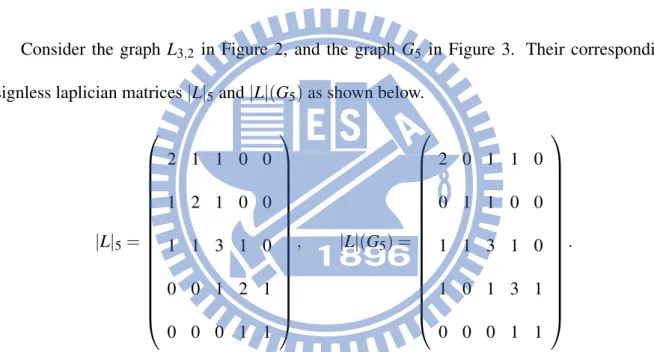
Consider the graph L3,2 in Figure 2, and the graph G5 in Figure 3. Their corresponding
signless laplician matrices|L|5and|L|(G5) as shown below.
|L|5= 2 1 1 0 0 1 2 1 0 0 1 1 3 1 0 0 0 1 2 1 0 0 0 1 1 , |L|(G5) = 2 0 1 1 0 0 1 1 0 0 1 1 3 1 0 1 0 1 3 1 0 0 0 1 1 .
L3,2 and G5have the same number of edges. We present another method to compare the least
eigenvalue of L3,2and G5. t 1 t 2 t 3 t4 t5
t 1 t 2 t 3 t 4 t5
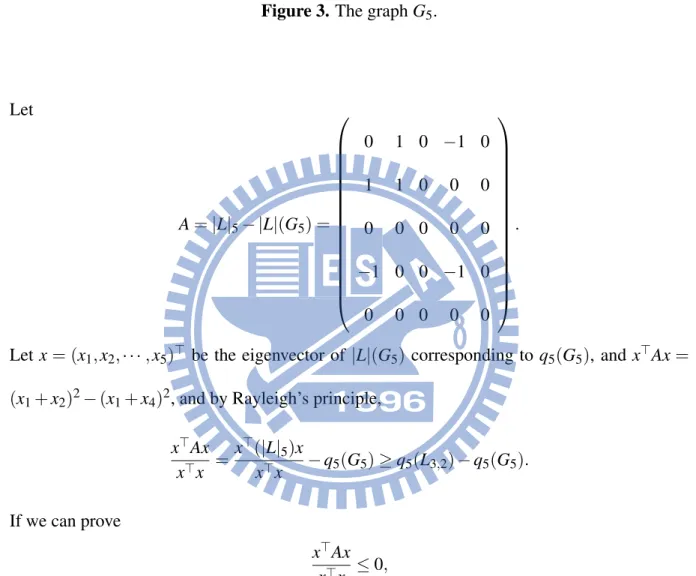
Figure 3. The graph G5.
Let A =|L|5− |L|(G5) = 0 1 0 −1 0 1 1 0 0 0 0 0 0 0 0 −1 0 0 −1 0 0 0 0 0 0 .
Let x = (x1, x2,··· ,x5)⊤ be the eigenvector of |L|(G5) corresponding to q5(G5), and x⊤Ax =
(x1+ x2)2− (x1+ x4)2, and by Rayleigh’s principle,
x⊤Ax x⊤x = x⊤(|L|5)x x⊤x − q5(G5)≥ q5(L3,2)− q5(G5). If we can prove x⊤Ax x⊤x ≤ 0,
then q5(L3,2)− q5(G5)≤ 0, so q5(L3,2)≤ q5(G5). Thus we need to find the eigenvector of
|L|(G5) corresponding to q5(G5). This is not a good idea, because in this case computing by
Mathematica,
and
x⊤Ax x⊤x =
x⊤(|L|5)x
x⊤x − q5(G5) = 0.6056− 0.3820 = 0.2236 > 0.
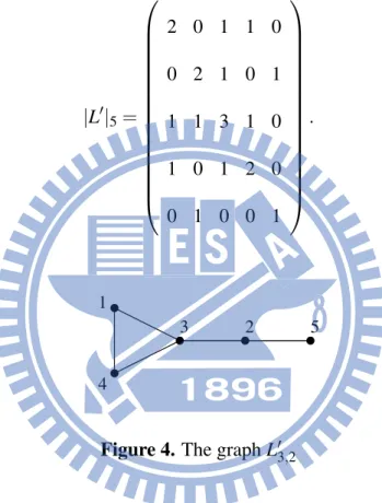
Now we try to change the symbols of vertices of L3,2, denoted by L′3,2. We switch the indices 2
and 4 as shown in Figure 4, so the new matrix is
|L′|5= 2 0 1 1 0 0 2 1 0 1 1 1 3 1 0 1 0 1 2 0 0 1 0 0 1 . t 1 t 4 t 3 t2 t5
Figure 4. The graph L′3,2
First we need a lemma.
Lemma 4.1. Let x = (x1, x2,··· ,x5)⊤ be the eigenvector of|L|(G5) corresponding to q5(G5).
Then|x2| = |x5| > |x3| = |x4|, and x1= 0.
Proof. Let q5be the least eigenvalue of|L|(G5), where G5is defined in Figure 3. Since deleting
the edge 45 in the graph G5yields L3,1, we have
q5≤ q4(L3,1) =
5−√17
by edge-interlacing in Proposition 3.7 and Example 2.2. By the definition of eigenvalue and eigenvector, 0 = (|L|(G5)− q5I)x = (2− q5)x1+ 0 + x3+ x4+ 0 0 + (1− q5)x2+ x3+ 0 + 0 x1+ x2+ (3− q5)x3+ x4+ 0 x1+ 0 + x3+ (3− q5)x4+ x5 0 + 0 + 0 + x4+ (1− q5)x5 .
Considering the second and fifth entries, and since q5< 1, we have
|x2| = | x3 q5− 1| > |x 3|, |x5| = | x4 q5− 1| > |x 4|, x2x4= x3x5.
Notice that any one of x2, x3, x4, x5 is zero will imply x = 0, a contradiction. Considering the
third and fourth entries, we have the following equations, step after step:
x1+ (3− q5)x3+ x4 = −x2, x1+ x3+ (3− q5)x4 = −x5, x1+ (3− q5)x3+ x4 x1+ x3+ (3− q5)x4 = x2 x5 = x3 x4 , x1x4+ x24+ (3− q5)x3x4 = x1x3+ x23+ (3− q5)x3x4, x1x4− x1x3 = x23− x24, x1(x4− x3) = (x3− x4)(x3+ x4), −x1 = (x3+ x4).
Considering the first entry, (2− q5)x1+ x3+ x4= 0, and by−x1= (x3+ x4), we have (2−
q5)x1− x1 = 0, and then (1− q5)x1= 0. Since (1− q5)̸= 0, we conclude that x1= 0. This
Let A′=|L′|5− |L|(5G) = 0 −1 0 1 0 −1 −1 0 0 0 0 0 0 0 0 1 0 0 1 0 0 0 0 0 0 ,
and as before let x = (x1, x2,··· ,x5)⊤ be the eigenvector of |L|(G5) corresponding to q5(G5).
Then x⊤(|L′|5)x x⊤x − q5(G5) = x⊤A′x x⊤x = (x1+ x4)2− (x1+ x2)2 x⊤x . Hence 0 > (x4) 2− (x 2)2 x⊤x = (x1+ x4)2− (x1+ x2)2 x⊤x = x⊤(|L′|5)x x⊤x − q5(G5)≥ q5(L ′ 3,2)− q5(G5).
Since q5(L3,2) = q5(L′3,2), we have the following Lemma.
Lemma 4.2. q5(L3,2) < q5(G5).
If we extend the definition of G5 to the graph Gn of order n by adding more vertices
6, 7, . . . , n and edges 56, 67, . . . , n− 1 n, then generalized the above arguments, one can show that qn(L3,n−3) < qn(Gn). Because the matrix B =|L|n− |L|(Gn) is the principal submatrix of
A, x⊤Bx is the same of above result, so qn(L3,n−3) < qn(Gn).
4.2
The largest eigenvalue
We shall study the largest signless laplacian eigenvalue q1(L3,n−3) of L3,n−3in this section. We
(i) q1(L3,n−3)≤ max{d(vi) + d(vj) : vivj∈ E(L3,n−3)} : d(v1) + d(v2) = 4, d(v2) + d(v3) = 5 = d(v1) + d(v3), d(v3) + d(v4) = 5, d(v4) + d(v5) = 5 = d(vi) + d(vi+1) f or 4≤ i ≤ n − 2, d(vn−2) + d(vn−1) = 4, d(vn−1) + d(vn) = 3. So q1(L3,n−3)≤ 5. (ii) q1(L3,n−3)≤ max{m(vi) + d(vi) : vi∈ V(L3,n−3)} :
Since m(v) =∑u∈N(v)d(u)d(v)
m(v1) + d(v1) = d(v2) d(v1) +d(v3) d(v1) + d(v1) = 5 2+ 2 = 9 2 = m(v2) + d(v2), m(v3) + d(v3) = d(v1) d(v3) +d(v2) d(v3) +d(v4) d(v3) + d(v3) = 2 + 3 = 5, m(v4) + d(v4) = d(v3) d(v4) +d(v5) d(v4) + d(v4) = 5 2+ 2 = 9 2, m(v5) + d(v5) = d(v4) d(v5)+ d(v6) d(v5)+ d(v5) = 2 + 2 = 4, m(v5) + d(v5) = m(vi) + d(vi) f or 5≤ i ≤ n − 2, m(vn−1) + d(vn−1) = d(vn−2) d(vn−1)+ d(vn) d(vn−1)+ d(vn−1) = 3 2+ 2 = 7 2, m(vn) + d(vn) = d(vn−1) d(vn) + d(vn) + 1 = 2 + 1 = 3.
So q1(L3,n−3)≤ 5.
(iii) q1(L3,n−3)≤ max{d(vi) + d(vj)− |Ni∩ Nj| : 1 ≤ i < j ≤ n,vivj∈ E(L3,n−3)} :
d(v1) + d(v2)− |N1∩ N2| = 4 − 1 = 3, d(v2) + d(v3)− |N2∩ N3| = 4 = d(v1) + d(v3)− |N1∩ N3|, d(v3) + d(v4)− |N3∩ N4| = 5, d(v4) + d(v5)− |N4∩ N5| = 5 = d(vi) + d(vi+1)− |Ni∩ Ni+1| f or 4 ≤ i ≤ n − 2, d(vn−2) + d(vn−1)− |Nn−2∩ Nn−1| = 4, d(vn−1) + d(vn)− |Nn−1∩ Nn| = 3. So q1(L3,n−3)≤ 5.
(iv) q1(G)≥ ∆(G) + 1 : We have q1(L3,n−3)≥ ∆(L3,n−3) + 1 = 4 in this case.
From the above discussing, we conclude that 4≤ q1(L3,n−3)≤ 5. By using edge-interlacing
in Proposition 3.7, a better lower bound of the least eigenvalue of|Ln| will be found. Since
q1(L3,1) =5+ √ 17 2 by example 2.2, we have 5 +√17 2 ≤ q1(L3,n−3)≤ 5.
q1(L3,1) q1(L3,2) q1(L3,3) q1(L3,4) q1(L3,5) q1(L3,6) q1(L3,7)
4.5616 4.6412 4.6554 4.6582 4.6588 4.6589 4.6590
These numbers are close to 4.66.
4.3
Characteristic polynomial
One way to study eigenvalues of a matrix is to compute the characteristic polynomial of the matrix and determine its roots. Let
|L|n= 2 1 1 0 ··· 0 0 0 1 2 1 0 . .. 0 0 0 1 1 3 1 . .. 0 0 0 0 0 1 2 . .. 0 0 0 .. . . .. ... ... ... 1 0 0 0 0 0 0 1 2 1 0 0 0 0 0 0 1 2 1 0 0 0 0 0 0 1 1 , Bn= 2 1 1 0 ··· 0 0 0 1 2 1 0 . .. 0 0 0 1 1 3 1 . .. 0 0 0 0 0 1 2 . .. 0 0 0 .. . . .. ... ... ... 1 0 0 0 0 0 0 1 2 1 0 0 0 0 0 0 1 2 1 0 0 0 0 0 0 1 2 be an n× n matrix for n ≥ 3. Note that Bn=|L|n+ Enn, where Enn is the binary matrix with a
Example 4.3. B3:= 2 1 1 1 2 1 1 1 3 , B4= 2 1 1 0 1 2 1 0 1 1 3 1 0 0 1 2 , B5= 2 1 1 0 0 1 2 1 0 0 1 1 3 1 0 0 0 1 2 1 0 0 0 1 2 .
Let Pn(λ) and Fn(λ) be the characteristic polynomial of|L|nand Bn, respectively.
Lemma 4.4. Pn(λ) = (λ− 1)Fn−1(λ)− Fn−2(λ) for n≥ 5.
Proof. Note that
Pn(λ) = det λ− 2 −1 −1 0 ··· 0 −1 λ− 2 −1 0 ··· 0 −1 −1 λ− 3 −1 ··· 0 0 0 −1 λ− 2 . .. 0 .. . ... ... . .. . .. −1 0 0 0 0 −1 λ− 1 n×n .
We expand about the determinant according to the nth column: Pn(λ) = (λ− 1) det λ− 2 −1 −1 0 ··· 0 −1 λ− 2 −1 0 ··· 0 −1 −1 λ− 3 −1 ··· 0 0 0 −1 λ− 2 . .. 0 .. . ... ... . .. . .. −1 0 0 0 0 −1 λ− 2 n−1×n−1 −(−1) det λ− 2 −1 −1 0 ··· 0 −1 λ− 2 −1 0 ··· 0 −1 −1 λ− 3 −1 ··· 0 0 0 −1 λ− 2 . .. 0 .. . ... ... . .. . .. −1 0 0 0 0 0 −1 n−1×n−1
= (λ− 1) det λ− 2 −1 −1 0 ··· 0 −1 λ− 2 −1 0 ··· 0 −1 −1 λ− 3 −1 ··· 0 0 0 −1 λ− 2 . .. 0 .. . ... ... . .. . .. −1 0 0 0 0 −1 λ− 2 n−1×n−1 − det λ− 2 −1 −1 0 ··· 0 −1 λ− 2 −1 0 ··· 0 −1 −1 λ− 3 −1 ··· 0 0 0 −1 λ− 2 . .. 0 .. . ... ... . .. . .. −1 0 0 0 0 −1 λ− 2 n−2×n−2 . Hence we have Pn(λ) = (λ− 1)Fn−1(λ)− Fn−2(λ).
Next we derive a recurrence relation for Fn(λ)
Proof. Note that Fn(λ) = det λ− 2 −1 −1 0 ··· 0 −1 λ− 2 −1 0 ··· 0 −1 −1 λ− 3 −1 ··· 0 0 0 −1 λ− 2 . .. 0 .. . ... ... . .. . .. −1 0 0 0 0 −1 λ− 2 n×n .
We expand about the determinant according to the nth column:
Fn(λ) = (λ− 2) det λ− 2 −1 −1 0 ··· 0 −1 λ− 2 −1 0 ··· 0 −1 −1 λ− 3 −1 ··· 0 0 0 −1 λ− 2 . .. 0 .. . ... ... . .. . .. −1 0 0 0 0 −1 λ− 2 n−1×n−1
−(−1) det λ− 2 −1 −1 0 ··· 0 −1 λ− 2 −1 0 ··· 0 −1 −1 λ− 3 −1 ··· 0 0 0 −1 λ− 2 . .. 0 .. . ... ... . .. . .. −1 0 0 0 0 0 −1 n−1×n−1 = (λ− 2) det λ− 2 −1 −1 0 ··· 0 −1 λ− 2 −1 0 ··· 0 −1 −1 λ− 3 −1 ··· 0 0 0 −1 λ− 2 . .. 0 .. . ... ... . .. . .. −1 0 0 0 0 −1 λ− 2 n−1×n−1 − det λ− 2 −1 −1 0 ··· 0 −1 λ− 2 −1 0 ··· 0 −1 −1 λ− 3 −1 ··· 0 0 0 −1 λ− 2 . .. 0 .. . ... ... . .. . .. −1 0 0 0 0 −1 λ− 2 n−2×n−2 . Hence we have Fn(λ) = (λ− 2)Fn−1(λ)− Fn−2(λ).
Lemma 4.6.
Pn(λ) = (λ− 2)Pn−1(λ)− Pn−2(λ) for n≥ 6,
where initial functions are
P4(λ) = λ4− 8λ3+ 19λ2− 16λ+ 4,
P5(λ) = λ5− 10λ4+ 34λ3− 48λ2+ 27λ− 4.
Proof. The initial functions are computed in Example 2.2. In general for n≥ 6,
Pn(λ) =(λ− 1)Fn−1(λ)− Fn−2(λ) (Lemma 4.4)
=(λ− 1)[(λ− 2)Fn−2(λ)− Fn−3(λ)]− [(λ− 2)Fn−3(λ)− Fn−4(λ)] (Lemma 4.5)
=(λ− 2)[(λ− 1)Fn−2(λ)− Fn−3(λ)]− [(λ− 1)Fn−3(λ)− Fn−4(λ)] =(λ− 2)Pn−1(λ)− Pn−2(λ) (Lemma 4.4).
From the above recurrence relation, we obtain the following two theorems.
Theorem 4.7.
(i) 1 is an eigenvalue of|L|nfor n≥ 4.
(ii) 2 is an eigenvalue of|L|nfor even n≥ 4.
(i) This follows from P4(1) = P5(1) = 0 and the recurrence of Pn(x) in Lemma 4.6.
(ii) This follows from P4(2) = 0 and the recurrence of Pn(x) in Lemma 4.6.
Lemma 4.8. For4≤ n ≡ 0 (mod 3), 1 is an eigenvalue of |L|nwith multiplicity at least 2, and
for 4≤ n ̸≡ 0 (mod 3), 1 is a simple eigenvalue of |L|n.
Proof. Computing the derivatives of P4(λ), P5(λ) and Pn(λ) in Lemma 4.6,
P4′(λ) =4λ3− 24λ2+ 38λ− 16, P5′(λ) =5λ4− 40λ3+ 102λ2− 96λ+ 27, Pn′(λ) =Pn−1(λ) + (λ− 2)Pn−1′ (λ)− Pn−2′ (λ). Since Pn−1(1) = 0, we have P5′(1) =− 2, P4′(1) =2, Pn′(1) =− Pn−1′ (1)− Pn−2′ (1), (1) P6′(1) =− P5′(1)− P4′(1) =−(−2) − 2 = 0. We prove by induction on k≥ 2 that
P3k′ −1(1) =− P3k′ −2(1)̸= 0,
This is true for k = 2. Suppose k > 2. Then by (1) and induction,
P3k′ −2(1) =− P3k′ −3(1)− P3k′ −4(1) =−P3k′ −4(1)̸= 0,
P3k′ −1(1) =− P3k′ −2(1)− P3k′ −3(1) =−P3k′ −2(1)̸= 0,
P3k′ (1) =− P3k′ −1(1)− P3k′ −2(1) = 0.
Theorem 4.9. For n≡ 0 mod 3, n ≥ 4, |L|nhas n− 1 distinct eigenvalues, and the eigenvalue
1 has multiplity exactly 2.
Proof. For any n≥ 4, since the diameter of L3,n−3is n−2, it has at least n−2+1 = n−1 distinct
eigenvalues[4]. In the case n≡ 0 mod 3, the eigenvalue 1 of |L|n has multiplicity at least two
by the above theorem, so|L|n has exactly n− 1 distinct eigenvalues, and the eigenvalue 1 has
multiplity exactly 2.
From Theorem 4.9, the following problem is raised.
Problem 4.10. Determine the integer n≥ 4 such that the graph L3,n−3 has n distinct signless
laplcian eigenvalues.
Example 4.11. Compute by Mathematica, we have the spectrum of|L|nfor 4≤ n ≤ 7:
|L|4 : { 5−√17 2 , 1, 2, 5 +√17 2 }; |L|5 : {0.2243,1,1.4108,2.7237,4.6412}; |L|6 : {0.1338,1,1,2,3.2108,4.6554}; |L|7 : {0.0884,0.7147,1,1.5710,2.4798,3.4877,4.6582}.
One might expect the answer of Problem 4.10 is n̸≡ 0 (mod 3). We leave the proof or disproof of this problem to successors.
References
[1] Weisstein, Eric W., Algebraic Connectivity, From MathWorld–A Wolfram Web Resource.
[2] Diestel, Reinard, Graph Theory, Grad. Texts in Math, Springer, ISBN 978-3-642-14278-9, 2005.
[3] Asratian, Armen S., Denley, Tristan M. J., H¨aggkvist, Roland, Bipartite Graphs and their
Applications, Cambridge Tracts in Mathematics 131, Cambridge University Press, ISBN
9780521593458, 1998.
[4] Andries E. Brouwer, Willem H. Haemers, Spectra of graphs, Springer, ISBN 978-1-4614-1939-6, 2011.
[5] Domingos M. Cardoso, Dragoˇs Cvetkovi´c, Peter Rowlinson and Slobodan K. Simi´c, A sharp lower bound for the least eigenvalue of the signless Laplacian of a non-bipartite graph,
Linear Algebra and its Applications, 2770-2780, 2008.