Robust attitude control of spacecraft using sliding mode control and productive networks

This article was downloaded by: [National Chiao Tung University 國立交通大學] On: 28 April 2014, At: 06:12

Publisher: Taylor & Francis

Informa Ltd Registered in England and Wales Registered Number: 1072954 Registered office: Mortimer House, 37-41 Mortimer Street, London W1T 3JH, UK

International Journal of Systems Science

Publication details, including instructions for authors and subscription information: http://www.tandfonline.com/loi/tsys20

Robust attitude control of spacecraft using sliding mode

control and productive networks

J. C. CHIOU a , M.-C. HWANG a , S. D. WUF a & J. Y. YANG a a

Department of Control Engineering , National Chiao-Tung University , Hsinchu, Taiwan, Republic of China Fax: E-mail:

Published online: 03 Apr 2007.

To cite this article: J. C. CHIOU , M.-C. HWANG , S. D. WUF & J. Y. YANG (1997) Robust attitude control of spacecraft using sliding mode control and productive networks, International Journal of Systems Science, 28:5, 435-446, DOI: 10.1080/00207729708929405

To link to this article: http://dx.doi.org/10.1080/00207729708929405

PLEASE SCROLL DOWN FOR ARTICLE

Taylor & Francis makes every effort to ensure the accuracy of all the information (the “Content”) contained in the publications on our platform. However, Taylor & Francis, our agents, and our licensors make no representations or warranties whatsoever as to the accuracy, completeness, or suitability for any purpose of the Content. Any opinions and views expressed in this publication are the opinions and views of the authors, and are not the views of or endorsed by Taylor & Francis. The accuracy of the Content should not be relied upon and should be independently verified with primary sources of information. Taylor and Francis shall not be liable for any losses, actions, claims, proceedings, demands, costs, expenses, damages, and other liabilities whatsoever or howsoever caused arising directly or indirectly in connection with, in relation to or arising out of the use of the Content. This article may be used for research, teaching, and private study purposes. Any substantial or systematic reproduction, redistribution, reselling, loan, sub-licensing, systematic supply, or distribution in any

form to anyone is expressly forbidden. Terms & Conditions of access and use can be found at http:// www.tandfonline.com/page/terms-and-conditions

Robust attitude control of spacecraft using sliding mode control

and productive networks

J.

C. CHIOUt, M.-C. HWANGt,

s.

D. Wut and

J.

Y. YANGt

A new robust attitude control design of spacecraft is proposed by combining sliding mode control (SMC) and productive networks (PN). Essentially, the sliding mode control uses discontinuous control action to drive state trajectories toward a specific hyperplane in the state space, and to maintain the state trajectories sliding on the specific hyperplane. This principle provides a guideline to design a robust controller. Productive networks, which are a special type ofartificial neural network, are then used to implement reaching and sliding conditions, and tackle the drawbacks ofSM Csuch as chattering and high control gains. A ttractive features of the proposed method include a systematic procedure of controller design, a reduction in chattering, robustness against model uncertainties and external disturbances. An inverted pendulum and a spacecraft attitude control problem are given to deomonstrate the effectiveness of the proposed method.

1. Introduction

Nonlinear control design has been studied for the last two decades (DeCarlo et al. 1988,Li and Slotine 1987, Sira-Ramirez and Dwyer 1987,Mamdani 1974,Narendra and Parthasatathy 1990). The aim of this research was to develop an analysis and design methodology that can possess robustness properties even in presence of parameter or structure uncertainties and disturbances. In the past, the application of nonlinear control methods was limited by the computational difficulty associated with nonlinear control design and analysis, such as the necessity of high speed and high precision. In recent years, however, advances in computer technology have greatly relieved this problem. Therefore, there is now consider-able enthusiasm for the research and applications of nonlinear control methods.

The sliding mode control was originally developed based on the variable structure system (VSS) control (Utkin 1977, DeCarlo 1988).It is known as a robust control to deal with confined uncertainties due to the modelling error and disturbances. The sliding mode control has been applied to many practical systems, such

Received 17 July 1996. Accepted 18 September 1996.

tDepartment or Control Engineering, National Chiao-Tung University. Hsinchu, Taiwan. Republic or China. Fax:+88635715998. e-mail: [email protected].

as flight control systems, robotics manipulator (Slotine and Sestry 1983, Bailey and Arapostathis 1987), and spacecraft attitude control (Singh and Iyer, 1989, Elmali and Olgac 1992).

The principal objective of sliding mode control is to force the trajectory of the system to a desired surface, which is known as the sliding surface. The control laws are designed so that the system state trajectory will reach the sliding surface. Once the state trajectory is on the sliding surface, it is well-known that the system is insensitive to certain parameter variations and external disturbances.

Although sliding mode control theoretically shows excellent robustness properties in dealing with parameter uncertainty and disturbances, classical sliding mode control however, presents several undesired drawbacks that limit its practical implementation. First, the most serious problem is the phenomenon of chattering, which is caused by practical switching limits, i.e. the components cannot operate at an infinite frequency. Since the method involves extremely high control activity, it may thus excite high frequency dynamics that are neglected in the course of modelling. Secondly, the sliding mode control laws are always chosen to be large enough in order to suppress those uncertainties caused by the parameter variations and external disturbances. Thus, it always makes the sliding mode control (SMC) hard to physically imple-ment. Finally, the control design procedure and the online

002().7721/97srzoo©1997 Taylor&Francis Ltd.

436 J. C. Chiou et al.

Ifthe following condition is satisfied with the designed control input, a sliding mode does exist:

In Li and Slotine (1987), the MIMO sliding condition is given by

where the state vector x(t)ER", and the control vector

u(t)ER":In particular, for each coordinate of the control vector u, we associate a collection of real-valued continuous functions

{ut(t,

x), ui-(t, x), slx)}, i

=

I, 2, ... , m, such that the controlU is given by

(2)

(5) (3)

(4)

i= 1,2, ... ,m,

for all time. i= 1,2, ...,m Si(X)

=

0,

{

ut (t,

x) forSi(X)

>

0, u{t x)

=

, , Ui-(t,x) for slx)

<

0, where

is the ith switching surface.

Since a sliding mode is a motion constrained on a sliding surface, the sliding surface is designed such that the system response restricted to sex) = 0 has the desired behaviour, such as stability and tracking. With this in mind, let us assume that the output of (I) is of the form yet)

=

h(x(t» and that the problem at hand now is to find a feedback control law to force the output to track a desired signal y.(t). According to the previous discussion, the synthesis problem involves two steps: first, the selection of a switching function s whose zeros comprise a surface on which the restriction of the dynamics has the tendency to drive the error yet) - y.(t) asymptotically to zero; secondly, the design of a switching control (corresponding to the choice ofs)that makes the state trajectory reach and slide on the sliding surface. A key issue in SMC design is decided by the existence of sliding mode on the switching surface. Thus, designing the proper switching surface is the complementary key problem in SMC design.

Although general nonlinear sliding surfaces are possible, linear ones are more prevalent in SMC design. After the switching surface has been designed, the next important aspect of SMC design is guaranteeing the existence of a sliding mode. The Lyapunov stability criterion is then used to derive a sliding condition so that the sliding surface can be reached within a finite time. A suitable Lyapunov function, D, can be chosen as

calculation are tedious and complicated, especially when the dimension of system is increased or the structure of the system is highly nonlinear.

In order to overcome these drawbacks, we introduce productive networks into the sliding mode controller design. Productive networks (PN) are artificial neural networks which employ fuzzy logic inference mechanisms. Problems requiring inferencing with Boolean logic have been implemented in perceptrons or feedforward net-works (Bulsari and Saxen 1991 a). However, feedforward neural networks with sigmoidal activation functions cannot accurately evaluate fuzzy logic expressions using the T-norm. Productive networks proposed by Bulsari (1992) and Bulsari and Sax en (1991 b) can accurately perform elementary fuzzy logic operations. The pro-ductive network is much simpler than a feedforward neural network since the architecture of the PN was desired to avoid extensive training; in fact, it requires no training.Itwas shown that fuzzy logic inferencing could be performed in productive networks by manually setting the offsets. Thus, it is reliable since the function of each of the nodes in the network is known and understood.

The objective of the present paper is to report a new robust control algorithm combined with sliding mode control and productive networks. The pro-posed method is aimed at effectively reducing the phenomenon of chattering and the high control gain effect due to nonlinear compensation. It can easily be implemented without a tedious design procedure and calculation.

This paper is organized as follows. Section 2 presents a review of the sliding mode control for a general nonlinear system. An introduction to productive net-works is given in § 3, including the derivation of productive networks and how to perform the three basic logical operations, AND, OR and NOT. Section 4 presents a new robust control method based on the sliding mode control and productive networks. In this section, we first apply the SMC principle to the dynamic systems so that the robustness of uncertainties and disturbances will be obtained once the systems are on the sliding surface. Secondly, by defining the increase or decrease of control inputs using productive networks, a control law can be determined. Section 5 presents a single-input single-output (SISO) inverted pendulum problem and a multi-input multi-output (MIMO) spacecraft attitude control problem that illustrate the performance of the present control algorithm. Section 6 gives the final conclusions. '

which guarantees the transient time from the initial state to the sliding manifold. Equation (6) is more restrictive 2. Sliding mode control

Consider a control system of the form

x(t) = f(t,x,U), (I)

tT > 0 i

=

1,2, ... ,m (6)

That is, all sliding subconditions in (6) with respect to sliding variables s,(x). i

=

I, 2, ... , m, are required to be strictly satisfied at any time instant.

From the above derivations, sliding mode control algorithms have been successfully developed. However, there exist the following drawbacks. First, the sliding mode controllers inherently contain a high frequency behaviour, i.e. chattering, which may excite high frequency dynamics neglected in the course of modelling. Secondly, the magnitudes of the SMC control laws are always chosen to be large enough in order to suppress those uncertainties caused by the parameter variations and external disturbances. Thirdly, the control design procedure of the system and the online calculation are tedious and complicated, especially, when the dimension of the system is increased or the behaviour of system is highly nonlinear.

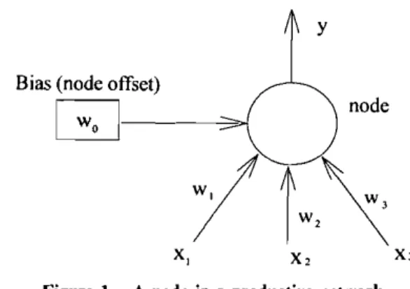
Figure I. A node in a productive network. node

X, X,

Bias (node offset)

[;]-~

t(A 1\ B 1\ C)

=

t(A)t(B)t(C) }

t(A v B v C)

=

I - (I - t(A»)(1 - t(B»)(1 - t(C) (14) for three operands. These operations contribute toward building the productive networks.

A productive network, as defined here, collects an offset product of inputs and a further offset by a bias. This can be illustrated by activation of the node as shown in Fig.

I, which can be written as

which is equivalent to the operation shown in (10). Similarly, we obtain the following operations:

(8)

(7)

for i

==

I, 2, ... , m. m • T' ' " • 0 v = s s

=

L. SiSj

< .

i=1

Note that (6) is a special case where than (5) which only requires

where the weights (WI'w₂₀w_{3 )} and bias(wo) are zero or one,Xi'i

=

1,2, 3 are the inputs of the node. The output ofthe node is the absolute value of the activation,a,i.e.

In general, one can express the activation in the following abbreviated form:

a= W_o

-I

I)

(w_j -

xjl

+(1/2)Wj(I-Wj))

I·

(17)

The productive network has multiple nodes with one or more inputs which should be positive numbers equal to or less than I. Each of the nodes has a bias (alternatively called the offset of the node). Obviously, the output is decided by the number between 0 and I. Productive networks are so named because of the multiplication of inputs at each node.

To show that the productive networks can be organized to compute any complicated logical operation, it is sufficient to show that the three basic logical operations can be implemented in this framework.

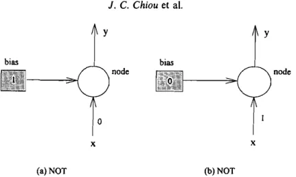
The simplest operation, NOT, can be represented by the networks shown in Fig. 2.

The AND operation as given in Fig. 3 is also implemented in a facile manner in this framework. Its 3. Productive networks

Since the aforementioned SMC algorithm suffers various drawbacks in computer implementation, these have motivated us to look for an alternative procedure that overcomes these difficulties. This alternative uses the productive networks to implement reaching and sliding conditions of SMC, and thus reduces the above-mentioned drawbacks. In productive networks, if we assume all logical operations can be represented as the combinations of AND (1\), OR (v) and NOT (-) operations, and the truth value of events A, BandCare represented byt(A), t(B) and t(C) respectively, then the truth values of AND, OR and NOT can be carried out as follows:

t(A 1\ B) = t(A)t(B) (9)

t(A v B)

=

t(A)

+

t(B) - t(A)t(B) (10)

t( - A)= 1 - t(A). (II)

The OR operation can be modified to a suitable form by

A vB

=

-(-A 1\ -B) (12)

t(A v B)

=

1 - (I - t(A»)(1 - t(B», (13)

y

=

[n]. (16)

438 J. C.Chiou et al.

o

node node

x x

(a) NOT (b) NOT

Figure 2. Inverting an input in a productive network (NOT): (a) has the same function as (b).

wherexl(t)ER'",X2(t)ERo-mare the plant state vectors, andu(t)ERm,y ERmare system input and output vectors

respectively. The desired output isYd(t)ER".

As described in § 2, the first step of SMC design entails sliding surfaces so that the system dynamics follow a desired performance once the system state trajectory is on the sliding surfaces. Itcan easily be accomplished by choosing

o

, c,> 0,

o

o

s=

e+

ce= 0, c

=

Figure 3. AND.

o

0 C_m i

=

1, ... ,m (19)

where e

=

Y - Ydis the tracking error and cERmx mis a

diagonal positive matrix. Once the state trajectory is on the sliding surface, the desired output will be satisfied. Next, the objective of the sliding mode control is to design a control law such that the sliding condition is satisfied i.e. equation (7) is satisfied. In this regard, we differentiate (19) with respect to time

once

and introduce (1) to obtain

Figure 4. OR.

s

=

e

+

ce

value of y is the product of the truth values of its arguments; i.e. both the weights and the bias have values of zero.

On the other hand, the OR operation requires all weights and bias equal to I. Figure 4 illustrates an OR

operation with ninputs in a productive network. (20)

where 4. Proposed nonlinear control algorithm

A MIMO nonlinear control system is taken as: X,

=

flex"~

x 2, t)

1

X2 = _{f2(x l, X2' t)}

+

_{G(x l, X2' t)u} Y

=

hex,) (18) B(x" x 2, t)=

(~).

_{(Ofl )'G(X" x 2, t)} oXI OX2

and [O.T] denotes the other terms. In the present development, equation (8) is used to perform a reaching and sliding condition because with equation (8) it is easier

to obtain the control rules than with equation (7), i.e. the condition

The final value of /iUj is obtained by the total summation of/iUijwith respect to each sliding surface, i.e.

i

=

1,2, ... , m, m

su,

=

L

so;

i=l j= 1,2, ...,m (26) (21) should be satisfied for each sliding surface. Now we can discuss the causal nexus betweenu)and S;,5;to construct control laws.

In equation (20), it is assumed that 5; increases as u)

increases and vice versa. Assuming B

_u

is greater than zero, equation (21) provides the information that ifs, is

greater than zero and 5; is greater than zero, then decreasing u)will result in decreasingS;5;.Ifs, is less than

zero and 5iis less than zero, then increasingu) will result

in decreasingS;5i'The inputs of the proposed productive networks controller with respect to the ith sliding surface are

s,

and 5;. The output in this development is_tJ.ui)which is the change ofu)with respect to the ith sliding surface.

In implementation, 5;is approximated with

(:I - :I-,

)IT

where

Tis

the sampling time. If we define the truth values of s,

>

0, 5;

>

0 as in Fig. 5, then the truth value of (increasing _MJu)is equal totees;

<

0) ("\(5i

<

0)] and the truth value of (decreasing_tJ.Uu) is equal to t[(Si

>

0) ("\ (5i

>

0)]. It is natural to choose the difference between t(increasingtJ.U;)and t(decreasing _/iUi) as actual output /iUij. In mathematical descriptions, we have

t(decreasing/iU;j)

=

tees;

>

0) ("\ (5;

>

0)]

= tees;

>

0)] . t[(5;

>

0)] (22) t(increasing/iU,j)

=

t[(s,

<

0) ("\(5i

<

0)]

=

t[~(s,:>0)] .t[~(5;

>

0)] (23) /iUij= t(increasing_{/iUij) _.} t(decreasing /iU;). (24)

If Bij is less than zero, according to the above discussion, the sign of_/iUushould be changed. Then we come to the conclusion that

/iUu= sign_(Bu)'[t(increasing_/iUu)

- t(decreasing _{/iUu)]. (25)}

Figure 5. Trutb value ofA>O.

and

Su,= k 3j · /i Uj j = 1,2, ... ,m (27) where kjs are prescribed given constants.

A systematic procedure is now available for robust control of nonlinear dynamic systems. The proposed nonlinear control algorithm is summarized as follows.

Step I. Design sliding surfaces,s,which are given in (19), such that the system response is restricted to s

=

0, which guarantees a desired behaviour such as stability or tracking. Initially, SO

=

0 and UO= 0 where upper index 0 denotes the initial

time step.

Step2. At a time step tp, computesP,and sp.

Step3. Evaluate these truth values ofsP

>

0,sP

>

0 with two factor vectors k ; k2 respectively.

Step4. Use equations (25) and (26) to compute the value of change of the ith control input with respect to each sliding surface.

Step 5. To evaluate the output ofthe controller, equation (27) is used and the control action is updated by

tI

=

tI-,

+

Su.

Step6. Add control action in Step 5 to the nonlinear dynamic system (1).

Step 7. Return to Step 2.

5. Numerical examples 5.1. S1S0 Systems

An inverted pendulum system shown in Fig. 6 is used as a SISO example. A movable pole is joined to a vehicle by a pivot. The pole, which serves as an inverted pendulum, can be kept standing by moving the vehicle appropriately. Letwo, Xl and y, denote the coordinates of the pole, and 8 is the angular position of the pole deviated from the equilibrium position. The pendulum has mass m and length 2L, and the moment of inertia is 1= mL2_13.Let

X 2 and Y2 denote the coordinates of the vehicle with mass M. The control force,u, is applied to

the vehicle. The equation of motion is:

[

m2L2 . ' mLcos 8 ]

mgLsin(J - - - -cos 8Sin8.82 - ·u

.. M+m M+m

8=

.

[ m2L2 ] 1

+

mL2 - ---cos28 M+m

440 J. C. Chiou et aJ. of---=::::::=~---~ - 3.5g, 15em pendulum --- 50g, 50cm pendulum 20 60 50 10

e

40 (deg) 30 Mg

(x"Y,)

/

u

Figure 6. Diagram of an inverted pendulum.

o

0.1 0.2 0.3 0.4 0.5 0.6 0.7 0.8 0.9 1.0

Time (sec)

Figure7. Time responses of Ott)of two different pendulums.

- - 3.5g,IScm pendulum ---. 50g, 50em pendulum

Since the goal of an inverted pendulum is to keep the pole standing, the actual output of the system and the desired output, Yd' are chosen to be

y(t)

=

0,

Yit) = O. The sliding surface, s,is chosen to be

S

=

0

+

JOO

=

O.

These two factors for t(s

>

0) and t(s

>

0) are k, and k₂

respectively.

Two pendulums with different lengths and weights are used for simulation. Their specifications are as follows:

pendulum No. I:3·5 g, IScm, pendulum No.2: 50 g, 50 ern.

12 10II \ 8

r\

6 \ S \ 4 \ 2 0 -2 0 0.2 0.4 Time (sec) 0.6 0.8 1.0 Td= 10 sin (200t).

The mass of the vehicle is I kg, which is the same for the two different pendulums. The resulting control was simulated for the following parameter values:

Time responses of the angular position for both pendulums, from the given initial condition of 60° from the equilibrium position, are shown in Fig. 7. The two response are almost identical in spite of the difference in system parameters, i.e. the system uncertainties. Note that there is no overshooting observed for both cases. The simulation results in Fig. 8 show the time responses of s.

In order to demonstrate the external disturbance rejection capability of the proposed method, a sinusoidal external force is applied on the vehicle in the horizontal direction. It is chosen as

Figure 8. Time responses of s(t)of two different pendulums.

Figures 9-11 show the simulation results. Pendulum No. 2 is used for both cases in order to make a comparison. The angular position response shown in Fig. 9 is almost unaffected by the external disturbance, although the time response of S as shown in Fig. 10 exhibits a severe

oscillation along the sliding surface.

Chattering is a serious drawback of sliding mode control and has been an important problem in the field of SMC. Figure 12 shows the state trajectory. It is clear that the phenomenon of chattering is greatly reduced.

In order to show how the proposed method performs better than that of SMC combined with fuzzy logic control (FSMC), we compare it with the method proposed by Hwang and Lin (1992). The system parameters are the same. Figures 13 and 14 show the simulation results. FSMC uses a 'two-degree nested control window' structure, in which the same set of control rules is used recursively and different scaling k,

=

10,

c

=

10,

k2

=

300,

70,---~---~-. - - without disturbance -.. ---. with disturbance 1.2 1.0 0.8 0.2

o

- ... ---. sliding surface

-~- 50g, 50cm pendulum

I

I~

II

-,

_/

"\::-

1/

.

o

0.4 0.6

e

(rad)

Figure 12. State trajectory of pendulum No.2.

-2 -8 -6

e

(rad/sec) -4 0.9 0.8 0.6 0.7 0.4 0.5 Time (sec) 0.3 0.2 0.1

o

10 20 40

a

(deg) 30

Figure 9. Time response of Ott) with disturbance.

4 2 12 ,---~-~-~~-~.-~-~~-~-0.9 0.8 0.7 - - proposed method --- ••••• FSMC

~

"":

t-:...::::.", .5 0.6 0.7 O. 0.2 0.3 0.4. Q.5) 0.6 Time (sec 0.1 50

e

40 (deg)30 20 10

o

- I.

~___::__:__-::-:___::-=---=--:--___::-=--__::_:____::-=-__::_:_----::--,---o

- - without disturbance --- with disturbance 0.1 0.2 0.3 0.4 0.5 0.6 0.7 0.8 0.9 1.0 Time (sec) ~ , ' \ " '\ '\ '\ ,. " I '\ 1\" {1\ "\ '\ "\r.f (.I .( f.1\ .'\ J oJ v 'J ' I . '/ \'v1} \: " ....J J \,I' V", \f", Ct 'oJ

o

-2."---;:-:---::'-:'-::--:---::-=--=-::---:e--:---:!-::---:--:--...,----,

o

8 6 10

Figure 10. Time response of s(t) with disturbance. Figure 13. Time responses ofOtt)of two different methods.

300,---~-~--.---~--~~-~-~-~---,

-100L-~_~_~~_ _~ _ ~ ~ _ ~ _ ~ _

o

0.1 0.2 0.3 0.4 0.5 0.6 0.7 0.8 0.9

Timetsec)

Figure 11. Time response ofuwith disturhance.

proposedmethod FSMC 0.7 0.8 0.9 0.3 100 50 o -50o,L-~~___::-=-___::_=_____:-,----::_=_====---:-::---=::::--:

Figure 14. Control inputs of two different methods.

350 300 ... with disturbance - - without disturbance 200

o

250 -50 150 ~100 50

442 J. C. Chiou et al.

For numerical simulation, the following values of the parameters of the spacecraft are assumed. The orbital angular speed,Wo, is 7·29 X 10- 5 rad S2. The modelling

Yd

=

[1 - e-o'353'(sin 0·353t

+

cos0'353t)]r where r

=

[180°,45°, 900]T.

The sliding surface is chosen to be

[

10 0]

[0,]

Y

=

0 1 0

°

=

h(O)

=

O2

o

0 1 03

o

o

~

«-»:

+

[~

=0. s=e+ce

The two factors required for t(s

>

0) and t(5

>

0) are k,

=

_{[k ll} k12 k'3]T

k

₂

=

[k 2, k22 k 23]T . (B) .

(a

f

li₎ sign ij

=

sign

aW

j [

0 cos 03 secO2 - sin 03 sec 02]

LlU

=

0 sin03 cos ₀₃

1 - tanO_{2 cos 03} tanO_{2 sin 03}

[

t[(s,

<

0) 1'1(5,

<

0)] - t[(s,

>

0)1'1(51

>

0)]] . t[(S2< 0) 1'1(52 < 0)] - t[(S2> 0) 1'1(52 > 0)]

t[(S3

<

0) 1'1(53

<

0)] - t[(S3

>

0) 1'1(53

>

0)]

u is the control torque vector and Td is the external disturbance vector. _{0= [0 1}O2 03]T denotes the roll, pitch and yaw angles about the body fixed axes respectively.

w[w,

W2 W2]T is the angular velocity with respect to the inertial frame, andW_{o, a constant, denotes} the orbital angular velocity of the mass centre of the spacecraft. (J, /2 /3) are the moments of inertia about the body fixed axes. The objective of this control strategy is to track Yd

=

[Old 02d 03d]T in the presence of modelling uncertainties and external disturbances. From Singh and Iyer (1989 and Elmali and Olgac (1992) we get

respectively. Note that B cannot be exactly obtained because the modelling uncertainties appear in the moments of inertia,

{Ii'

i = 1,2, 3}. Since we know the values of

{Ii>

i= 1,2, 3} are all positive, it means that the sign ofBijremains unchanged, i.e.

0 0 -Td, /, /, G= 0 0 _Td= Td2 /2 /2 0 0 'ld3 /3 /3

(.{:]

[

-",0.

00'

0,

]

= cos _{0, sin 03}

+

sin0, sinO_{2 cos 03 .}

cos _{0, cos 03 - sin 0, sin}O_{2 sin 03} 5.2. M/MO systems

The attitude control problem of a spacecraft is considered to be an exam pie of MI M0 nonlinear systems. Typically, dynamics and associated characteristics are taken from Singh and Iyer (1989) and Elmali and Olgac (1992). Assume the spacecraft is on a circular orbit in an inverse square gravitational field, and the attitude of the space vehicle has no effect on the orbit. The equations of motion of the system are

[

f ' l ] [COS03 sec

~2W2

- sin 03 sec 02W3 -

wo]

f,

=

f'2

=

sm03W2

+

cos03W3

f'3 W,

+

tan 02(sin03W3 - cos 03W2)

/2 - /3 2 - - - (W2W3 - 3WO~2~3) /, /3 - /, 2 f2 = _{- - ( W3W, -} 3WO~3~') /2

t, -

/2 2 --(W'W 2 - 3WO~'~2) /3

factors are used for each degree of nest. The scaling factors for the first degree of nest are chosen as the same as the proposed method: k ,

=

10, _k2

=

300 and _k3

=

40; the scaling factors for the second degree of nest are k, = 0'5,

k2

=

20 andk3

=

4. It is more tedious than the proposed method which only needs one set of the scaling factors. In order to avoid the time consumption on defuzzification of FSMC, it needs a look-up table which directly relates the controller inputs sand 5 with the controller output change Llu.This will cause control input to oscillate as, shown in Fig. 14. On the other hand, the control input of the proposed method yields no oscillatory effect at the closing stage of the simulation.

x,

=

f,(x)

X 2

=

fix)

+

Gu

+

Td

wherex

=

[x, X2]

=

[OT WT] is the state vector, and

where sat(Bij ) =

J

~ij

1-1

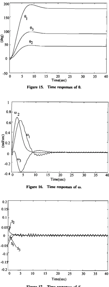
40 35 30 10 15 20 25 Time(sec) Figure 15. Time responses of 9.

5 -50 '---_~_~_~_~_~_~_~_ _____.J

o

0.8 00 2 0.6 ~0.4 il

~O2

0 -0.2 -0.4 0 10 15 20 25 30 35 40 Tirne(sec)

Figure 16. Time responses ofroo

0.2 0.\5 0.1 0.05

~~

0

1'>-..

,A "

~\

-0.0 ~ -0.1 -0.\ -0.2 0 5 10 \5 20 25 30 35 40 Time(sec)

Figure 17. Time responses ofS.

[

M I]

[VIII]

M₂

=

0·5[1

+

sin (O·lt)]- v₂I₂

flJ.I3

v3I3

where

VI

=

0·1,

V2

=

0·2,

V3

=

0·3. The external dis-turbances are chosen as

Td l

=

40 sin(2m)

T.s2

=

40 cos(2m) Td 3= 20 sin (2m).

Bound.j

=

III

Boundv, = [cos 83sec 821

Bound.j

=

[sin0₃sec 8₂1

Boundy,

=

III

Boundy; = [sin 031

Boundy,

=

[cos 831

Boundj ,

=

III

Boundy, = [tan 82cos 831 Boundj , = [tan 82sin 83

1.

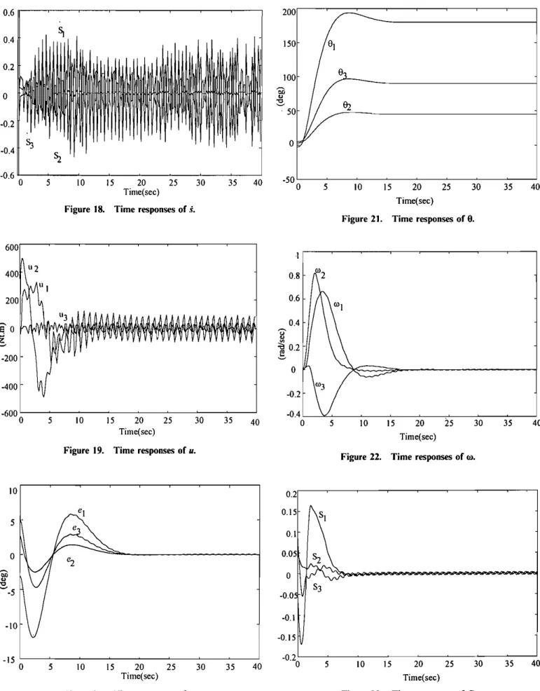
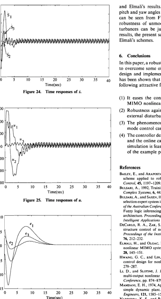
Simulation results on the attitude tracking manoeuvres are shown in Figs 21 and 22. In accordance with the sliding-mode theory, Figs 23 and 24 illustrate that the sliding vectors sand Sare driven to the sliding surface and then stayed oscillatory because of the desired tracking variablesYd. All of the control torques applied in Figs 19, 20, 25 and 26 show that the present scheme requires lesser torques in comparison with both Singh uncertainties appear in the form of I,

+

flJ.I"

i= 1, 2, 3, where II

=

874·6, 1₂

=

888·2 and 1₃

=

97·6 kg m2. The variations in the inertia are taken as

The initial orientation of the spacecraft is taken as 8₀

= [-

3 3 5]Tdegrees. Simulation of the closed-loop system with control design parameters is chosen as follows: c

=

diag (I, I, I), k ,

=

[0·1 0·1 O·lY, k2 = [0·1 0·1 O·lY and k3 = [I I I]T. The responses of spacecraft are shown in Figs 15 and 16. The transition of the error functions with tracking conditions are stabilized in nearly 20 s, as shown in Figs 19 and 20, whereas, the time differentiation of sliding surfaces, S, experienced high frequency chattering behaviour as illustrated in Figs 17 and 18. In order to improve the behaviour, we further choose saturation function Bijas

ifBi j > Bound.,

ifBij

<

Bound., ifBij

< -

Bound.,

444

J. C. Chiou et al. 0.6 0.4 0.2 0

on

...

~ -0.2 -0.4 ~ -0.6 0 5 10 15 20 25 30 35 40 -50 Time(sec) 0 5 10 15 20 25 30 35 40

Figure 18. Time responses of

s.

Time(sec)

Figure 21. Time responses of O.

600 0.8 0.6 ~ 0.4

e

0 ~

~

tJ

...

~ ]. 0.2 0 -0.2 -600 -0.4 0 5 10 15 20 25 30 35 _{40 0 10 15 20 25 30 35 40} Time(sec) Time(sec) Figure 19. Time responses ofu.

Figure 22. Time responses of ro.

10 _0.2 0.15 SI 5 0.1 0 0.05

l~~

~ bJl ₀

...

'0 S3 ~-5 -0.0 -0.1 -10 -0.15 -0.2 -15 _{30 35 40} 0 5 10 15 20 25 30 35 40 0 5 10 15 20 25 Time(sec) Time(sec)

Figure 20. Time responses ofe. Figure 23. Time responses ofS.

0.2 0.4,---~-~-~-~·-~-~-~---, 0.3 lilA "" '~~~~M~~~MM••MMMMMM~MM~MM~~~~~. ~ v .~~ .~~~~.~~~~~ .~~~ .~~~~ .~~ \,. ~ 6. Conclusions

In this paper, a robust control scheme has been developed to overcome some of the difficulties encountered in the design and implementation of sliding mode control. It has been shown that the proposed scheme possesses the following attractive features.

and Elmali's results. The successful trace of the roll, pitch and yaw angles to the corresponding desired angles can be seen from Figs 19, 20, 25 and 26. Hence, the robustness of unmodelled dynamics and external dis-turbances can be justified. In view of the simulation results, the present scheme outperforms both Singh and Elmali's schemes. 40 35 30 10 15 20 25 Time(sec)

Figure 24. Time responses of

s.

5 0.1

o

-0.3 -0.1 -0.2 References

BAILEY. E., and ARAPOSTATHIS, A .. 1987, Simple sliding mode control

scheme applied to robot manipulators, International Journal of

Control, 45, 1197-1209.

BULSARI, A., 1992, Training artificial neural networks for fuzzy logic.

Complex Systems, 6, 443-457.

BULSARI, A .• and SAXEN, H., 1991a, Implementation of chemical reactor

selection expert system in a feedforward neural networks.Proceedings

ofthe Australian Conference on Neural Networks, pp. 227-229; 1991b,

Fuzzy logic inferencing using a specially designed neural network

architecture. Proceeding a/the International Symposium on Artificial

Intelligent Applications and Neural Networks, pp. 57-60.

DECARLO, R.A., ZAK, S. H., and MATTHEWS,G. P.•1988, Variable

structure control of nonlinear multi variable systems: a Tutorial.

Proceedings of the Instituteof Electrical and Electronics Engineers,

76,212-232.

ELMALI. H.,and OLGAe, N., 1992, Robust outpul tracking control of

nonlinear MIMO systems via sliding mode technique. Auromatica,

28,145-151.

HWANG, G. C, and LIN, S. C, 1992, A stability approach to fuzzy

control design for nonlinear systems. Fuzzy Sets and Systems, 48,

279-287.

LI. D .. and SLOTINE,J. J., 1987, On sliding control for multi-input multi-output nonlinear systems. Proceedings of the America Control

Conference, pp. 874-879.

MAMDANI, E. H., 1974, Applications of fuzzy algoritbms for control of simple dynamic plant. Proceedings of the Institute of Electrical Engineers, 121, 1585-1588.

NARENDRA, K. S., and PARTHASATATHY, K., 1990, Identification and

control of dynamical systems using neural networks. IEEE

Transactions on Neural Networks,1,4-27.

(I) It eases the controller design for both SISO and MIMO nonlinear dynamic systems.

(2) Robustness against the modelling uncertainties and external disturbances is obtained.

(3) The phenomenon of chattering, inherent in sliding mode control can be effectively reduced.

(4) The controller design procedure of the system is facile and the online calculation is simple, thus a real-time simulation is feasible in the physical implementation of the example problems.

40 40 35 35 30 30 25 15 20 Time(sec) 10 10 15 20 25 Time/sec)

Figure 25. Time responses of u.

5 5 -15L-_~_~_ _~ _ ~_ _~_ _~_~_---J

o

_600L--~-~-~--~--~-~-~_---J

o

5 -10

o

10 400

Figure 26. Time responses ofe.

-400 600r--~-~--~-~--~--~-~---; 200

?

~ -5

'Eo

g

-200

446

Robust attitude control of spacecraft

S,NGH, S. N., and IYER,A., 1989, Nonlinear decoupling sliding mode control and attitude control of spacecraft. JEEE Transactions on Aerospace Electronic Systems,25, 621-633.

SIRA-RAMIREZ, H., DWYER, III, T. A. W., 1987, Variable structure controller design for spacecraft nutation damping. IEEE Transactions

on Automatic Control,32, 435-438.

SLOTINE,J. J.,SASTRY, S. S.,1983,Tracking control of nonlinear systems using sliding surfaces, with application to robot manipulators.

International Journal oj Control, 38,465-492.

UTKIN,V. I., 1977, Variable structure systems with sliding modes. I EEE

Transactions on Automatic Control,22, 212-222.