以無線網路訊號量測強度為基礎之增加空間向度的定位演算法

國

立

交

通

大

學

電信工程研究所

碩

士

論

文

以無線網路訊號量測強度為基礎之增加空間向度的定位演算法

A Diversity-Augmented Location Estimation

Algorithm for RSS-Based Wireless Networks

研 究 生：林宥儒

指導教授：方凱田 教授

以無線網路訊號量測強度為基礎之增加空間向度的定位演算法

A Diversity-Augmented Location Estimation Algorithm

for RSS-Based Wireless Networks

研 究 生：林宥儒 Student：Yu-Ju Lin

指導教授：方凱田 Advisor：Kai-Ten Feng

國 立 交 通 大 學

電信工程研究所

碩 士 論 文

A Thesis

Submitted to Institute of Communication Engineering College of Electrical and Computer Engineering

National Chiao Tung University in partial Fulfillment of the Requirements

for the Degree of Master

in

Communication Engineering

August 2011

Hsinchu, Taiwan, Republic of China

以無線網路訊號量測強度為基礎之增加空間向度的定位演算法

學生：林宥儒

指導教授

：

方凱田

國立交通大學電信工程研究所碩士班

摘

要

近年來行動裝置(Mobile Station)的定位已經日漸備受注目，而且重

要性與日俱增。而建構在行動裝置和基地台 (Base Station) 網路架構上

的定位演算法已經被廣泛應用到各個層面。傳統上的兩步求最小平方法

(Two-Step Least Square) 之定位演算法，對於定位行動裝置來說，提供

了 一 個 很 有 效 率 的 解 法 。 而 另 一 個 以 幾 何 限 制 為 輔 助 之 定 位

(Geometry-Assisted Location Estimation) 演 算 法 ， 則 將 非 直 線 路 徑

(None-Line-of-Sight)雜訊造成的行動裝置和基地台之相對陳列關係加入

了考量。後者針對了超視距雜訊，在以前者為基礎上，多附加了幾何上的

限制，增加了定位上的精確度。無論如何，前述兩者都是以到達時間

(Time-of-Arrival) 作為量測基礎，而制定的演算法。很少有人以訊號量

測強度 (Received Signal Strength) ，這種很容易被今日各種行動裝置

取得的訊號來源，為基礎而來設計演算法。我們因而提出了一個以寬頻無

線 網 路 訊 號 量 測 強 度 為 基 礎 之 增 加 多 樣 性 的 定 位 演 算 法 (A

Diversity-Augmented Location Estimation Algorithm for RSS-Based

Wireless Networks)。此一演算法同時也考慮了路徑損耗指數(Path Loss

Exponent)對於訊號量測強度轉換到估測距離所造成的影響，因而採取機制

去修正它。我們所提出的演算法同時保留了兩步求最小平方法的優點，也

透過了訊號量測強度來做出良好而精確的定位估算。我們也提供了許多模

擬結果來證明所提演算法的效能的確能勝過許多已經存在的定位演算法。

A Diversity-Augmented Location Estimation Algorithm for RSS-Based Wireless Networks

Student：Yu-Ju Lin Advisors：Dr. Kai-Ten Feng

Institute of Communication Engineering National Chiao Tung University

ABSTRACT

Mobile location estimation has attracted a significant amount of attention in recent

years. The network-based location estimation schemes have been widely adopted

based on the radio signals between the mobile device and the base stations. The

two-step least square (TSLS) method has been studied in related research to provide

efficient location estimation of the mobile devices. In order to enhance the precision of

location estimate, the geometry-assisted location estimation (GALE) scheme is

designed to incorporate the geometric constraints within the formulation of TSLS

method. However, these two algorithms are mainly designed based on the

time-of-arrival (TOA) measurements. There is not much effort that has been dedicated

in location estimation based on received signal strength (RSS) measurements, which

can be easily obtained by mobile devices nowadays. A diversity-augmented location

estimation (DALE) algorithm is proposed in this thesis with additional spatial

assistance based on the RSS measurements. This algorithm also considers and corrects

the effect of incorrect path loss exponent (PLE). The proposed DALE scheme can both

preserve the computational efficiency from the TSLS algorithm and obtain precise

location estimation based on RSS measurements. Numerical results demonstrate that

the proposed DALE algorithm can achieve better accuracy, comparing with other

existing schemes, in mobile location estimation.

誌

謝

時光荏苒，回首二十五年的人生，二十年的求學生涯，佔了其中的八成。其中在交 大的六年，應該是最精彩的一段回憶。大學的四年，充滿了歡笑和淚水，從懵懂無知， 到瞭解自主學習的重要，也從初嚐愛情的甘甜，到明白分手的苦澀，自由自在的四年， 曾讓大家以為像一輩子一樣長久；轉瞬間大學畢業，大家各奔前程，許多好友抱著不同 的志向而離開，而我，直升上了研究所，並且很幸運地成為 MINT LAB 的一員。初次 和實驗室結緣，是在大學部的時候跟隨著老師做專題，那時候只是覺得老師對大家很好， 不會給予太大的壓力，讓大家可以自己掌握研究的進度；但是一直不能明白，為何每次 到實驗室做研究的時候，總是會看到許多學長們專心致志的在寫程式、看 paper，甚至 熱烈的討論，即使老師不常出現在實驗室。直到成為了這裡的一份子，才慢慢明白，這 就是所謂的桃李不言，下自成蹊吧！每次 meeting 的時候，老師總會很專心並且相當有 耐心地想要聽懂學生所表達的意思，並且給予豐富的回應，即使老師有時候往返國內外， 還是鮮少在老師身上看見倦容，而主持完每一次的 meeting，使學生都會有一些收穫和 方向。也許是因為老師的努力潛移默化了實驗室的前輩們，再由前輩們一直帶領著良好 的研究風氣，使得我們後進的新生會不自覺的也想好好的向上學期---不論是做研究還是 修習課業。除此之外，實驗室的夥伴們也時常在寒暑假舉辦出遊，所以大家的感情都很 融洽，而不會因為研究而有肅殺的壓力，讓我很享受待在這邊的日子。 由衷感謝 MINTers 夥伴們(仲賢、建華、志明、添壽、文俊、柏軒、佳仕、子皓、 林智、瑞廷、俊傑、其懋、俊宇、萬邦、承澤、瑞鴻、惟能、昭華、劭凱、裕平、修銘、 智偉、景維、治緯、唯慶)在我研究所時期的相伴，認識大家是我的福氣，我在每一個 人身上都看到了值得我學習的地方，你們同時是我的良師、益友，還有運動場上的好夥 伴。在實驗室的夥伴中，最感謝的是建華學長，他總是不厭其煩的把所知道的知識和我 分享，幫助我解決相當多推導演繹上的難題，也讓我見識到數學除了用在考試上之外， 在研究上也可以是使用得這麼得心應手的好工具。 人生將要邁入下一個階段，也許要暫時離開一陣子去從軍，但是將來退伍之後，希 望還是可以常回來看看老師、看看大家，聊聊以前的種種，分享畢業出社會後的所見所 聞和心得感想。祝福大家身體健康、學業精進、事業亨通，而友誼長存不忘。 林宥儒 謹誌 于新竹國立交通大學

Contents

Chinese Abstract i English Abstract ii Acknowledgement iii Contents iv List of Figures vi 1 Introduction 1 2 Related Work 4 3 Preliminary 7

3.1 Modeling of the Signal Measurements . . . 7 3.2 Least Square Methods for Location Estimation . . . 8 3.3 Overlapped Region of Three Range Measurements . . . 10

4 Proposed Diversity-Augmented Location Estimation Algorithm 13 4.1 Mechanism of Distance Estimation . . . 15 4.2 Mechanism of Range Adjustment . . . 18 4.3 Diversity-Augmented Location Estimation . . . 21

CONTENTS

5 Performance Evaluation 32

6 Conclusion 44

List of Figures

3.1 An illustration of outer separate and intersection of two range measurements 11 3.2 An illustration of intersections of two circles and overlapping of three circles 11 4.1 Flow chart of our proposed DALE algorithm . . . 14 4.2 An illustration of range measurements after RA mechanism and the result

of overlapped region . . . 22 4.3 An illustration of range adjustment and the projection of error variance . . 23 5.1 The relationship between PLE estimation error and noise standard

devia-tion in a regular triangle . . . 34 5.2 The relationship between location estimation error and noise standard

de-viation in a regular triangle . . . 35 5.3 The relationship between PLE estimation error and noise standard

devia-tion in an irregular triangle . . . 36 5.4 The relationship between location estimation error and noise standard

de-viation in an irregular triangle . . . 36 5.5 The relationship between PLE estimation error and noise standard

devia-tion in an arbitrary triangle . . . 37 5.6 The relationship between location estimation error and noise standard

LIST OF FIGURES

5.7 The comparison of location estimation error under the fading noise with 4 dB standard deviation in scenario S1 and S2 . . . 38 5.8 The comparison of mean squared error in the scenarios S1 and S2 . . . 40 5.9 The comparison of location estimation error under the fading noise with 4

dB standard deviation in scenario S3 and S4 . . . 40 5.10 The comparison of mean squared error in the scenarios S3 and S4 . . . 41 5.11 The comparison of location estimation error under the fading noise with 4

dB standard deviation in the scenario S5 . . . 42 5.12 Scenario 5’s MSE with respect to standard deviation . . . 43

Chapter 1

Introduction

Wireless location technologies, which are designated to estimate the position of a mobile station (MS), have drawn a lot of attention over the past few decades. Different types of location-based services (LBSs) have been proposed and studied, including the emer-gency 911 (E-911) subscriber safety services [1], the location-based billing, the navigation system, and applications for the intelligent transportation system (ITS) [2]. Due to the emergent interests in the LBSs, it is required to provide enhanced precision in the location estimation of a MS under different environments.

A variety of wireless location techniques have been studied and investigated [3], [4], [5]. The network-based location estimation schemes have been widely proposed and employed in the wireless communication systems. These schemes locate the position of the MS based on the measured radio signals from its neighborhood base stations (BSs). The representative algorithms for the network-based location estimation techniques are the time-of-arrival (TOA), the time difference-of-arrival (TDOA), and the angle-of-arrival (AOA). The TOA scheme estimates the MS’s location by measuring the arrival time of the radio signals coming from different wireless BSs; while the TDOA method measures the time difference between the arriving radio signals. The AOA technique is conducted within the BS by observing the arriving angles of the signals coming from the MS.

The equations associated with the network-based location estimation schemes are in-herently nonlinear. The uncertainties induced by the measurement noises make it more difficult to acquire the estimated MS position with tolerable precision. Algorithms applied least square (LS) such as the two-step least square (TSLS) scheme [6] has been studied to provide reasonable accuracy for location estimation with its efficient two-step calculation. However, the algorithms based on the TSLS method are primarily feasible for location estimation under line-of-sight (LOS) environments. The non-line-of-sight (NLOS) situa-tions, which occur mostly under urban or suburban areas, greatly affect the precision in most of the location estimation schemes. On the other hand, the range scaling algorithm (RSA) proposed in [7] alleviates the NLOS errors by considering the cell layout between the MS and its associated BSs. A constrained nonlinear optimization approach is adopted to obtain improved location estimate for the MS. However, the RSA approach involves the requirement of solving an optimization problem based on a nonlinear objective function. The inefficiency incurred by the algorithm may not be feasible to be applied in practical systems.

In this paper, an efficient Diversity-Augmented Location Estimation (DALE) algo-rithm is proposed to obtain location estimation of the MS based on received signal strength (RSS) measurements. The proposed DALE scheme integrates the spatial di-versity by combining additional constrains with the conventional TSLS algorithm. We retrieve the distance by using RSS measurements and the path loss model. Moreover, we take the jittering of path loss exponent (PLE) into consideration in the proposed DALE algorithm, which always happens due to the channel fadings. The MS’s position is ob-tained by correcting the PLE to reduce the error of Distance Estimation (DE) during the process of converting RSS into range measurements, then solving the equations with additional constrains in DALE. Different cases are illustrated in simulations in order to demonstrate the effectiveness of the proposed DALE algorithm. Comparing with other

existing schemes, numerical results show that the DALE approach can acquire higher accuracy for location estimation of the MS.

The remainder of this thesis is organized as follows. Chapter 2 describes the related work for wireless location estimation. In Chapter 3, we introduce the models of measure-ment signals and existing LS schemes as background knowledge. The proposed DALE algorithm is described in Chapter 4. The performance evaluation of proposed scheme is conducted in Chapter 5 via simulations. Chapter 6 draws the conclusions.

Chapter 2

Related Work

Different location estimation schemes have been proposed to acquire the MS’s position. Various types of information (e.g. the signal traveling distance, the received angle of the signal, or the RSS measurements) are involved to facilitated the algorithm design for location estimation. The primary objectives in most of the location estimation algo-rithms are to obtain higher estimation accuracy with promoted computational efficiency. The high-resolution (super-resolution) schemes are proposed as in [8], [9], [10], [11]. The scheme studied in [8] considers arbitrarily located antennas and a particular covariance matrix within a noisy environment. The covariance matrix is composed of various types of properties, including gain, phase, frequency, polarization, and angle-of-arrival (AOA) information. The subspace method utilized in the super-resolution schemes estimates the components of the covariance matrix based on an eigen-analysis. The well-known super-resolution algorithm is the multiple signal classification (MUSIC) [9]. It is experimentally illustrated to be a robust solution for location estimation, especially for a near-far envi-ronment. However, it has also be shown in [10] and [11] that the drawbacks of the MUSIC approach include (i) comparably high sensitivity to large noise and (ii) its complexity in computation.

sensor array. It provides spatial filtering capability which enhances the amplitude of a co-herent signal associated with the surrounding noises. Since the conventional beamforming technique is sensitive to the estimation error for the MS’s position, a combination of lo-calization and beamforming is proposed as in [12]. It increases the robustness to location errors without sacrificing the computation efficiency. An enhanced algorithm for simul-taneous multi-source beamforming and adaptive multi-target tracking is studied in [13]. The correlation between the adaptive minimum variance beamforming and the optimal MS localization is also investigated as in [14]. However, the complication of the beamform-ing system makes the associated location estimation techniques difficult to be practically realized.

Instead of exploiting the spatial and temporal information of the signal, the location fingerprinting technique locates the MS based on the RSS [15] [16]. The technique involves both the off-line and the on-line phases. A location grid that is related to a signal signature database for a specific service area is developed in the off-line phase; while a measured RSS vector at the MS is delivered to the central server to compare with the location grid in the on-line phase. Moreover, a hybrid algorithm which combines the RF propagation loss model is proposed both to mitigate the requirement of the training data and to adjust the configuration changes [17]. It is obvious to recognize that a considerable size of database is required for the location fingerprinting techniques.

There are also different approaches exploiting linearized methods to achieve computing efficiency while obtaining an approximate estimation of the MS’s position. The Taylor series expansion (TSE) method was utilized in [18] to acquire the location estimation from the TDOA measurements. The method requires iterative processes to obtain the location estimate from a linearized system. The major drawback of the TSE scheme is that it may suffer from the convergence problem due to an incorrect initial guess of the MS’s position. The TSLS method was adopted to solve the location estimation problem

from the TOA [6], the TDOA [19], and the TDOA/AOA measurements [20]. It is an approximate realization of the maximum likelihood (ML) estimator and does not require iterative processes. The TSLS scheme is advantageous in its computational efficiency with adequate accuracy for location estimation.

Instead of utilizing the circular line of position (CLOP) methods (e.g. the TSE and the two-step LS schemes), the linear line of position (LLOP) approach is presented as a new interpretation for the cell geometry from the TOA measurements. Since two TOA measurements that intersect at two points will generate a connecting line, two indepen-dent lines will be created by using three BSs in the scenario of two-dimensional location estimation. Therefore, the LS method can be adopted to estimate the location of the MS. The detail algorithm of the LLOP approach can be obtained by using the TOA measurements as in [21], and the hybrid TOA/AOA measurements in [22].

It can be found from the previous work that some of the location estimation algorithms involve complicated computation or additional database and infrastructures; while others are only suitable for specific situations (e.g. LOS environments or special areas). Not much effort has been dedicated in location estimation based on RSS with light off-line database construction. The DALE algorithm based on RSS measurements as proposed in this paper preserves the computational efficiency from the TSLS method; while reducing the requirement of hardware’s capability of transmitting and measuring.

Chapter 3

Preliminary

In this chapter, the mathematical modeling of the signal measurements is formulated in the Section 3.1. The conventional linear LS methods for location estimation is briefly reviewed in the Section 3.2. Moreover, the range measurements converting from the observations of RSS may suffer from unreasonable geometric relationships as the log-normal distributed fading effects exists. Thus, in Section 3.3, the overlapped region among three range measurements is denoted and emphasized.

3.1

Modeling of the Signal Measurements

In order to facilitate the design of the proposed DALE algorithms, the signal model for the RSS measurements is presented in this Section. To describe the model precisely, we have surveyed some technical reports and documents. The COST 231 [23] project is a com-prehensive framework in which the radio channel characteristics for various environments are investigated and developed. Furthermore, the advancements for E-UTRA physical layer aspects [24] are continuously moving in in the 3GPP technical specifications. It also provides path loss models for various propagation scenarios which have been adopted in the paper. Some simulation assumptions and parameters in [25] are suggested to describe

the interferences between macrocells and femtocells in LTE and so as the path loss models in different scenarios.

According to the model suggested in [24], the indoor path loss model can be expressed as

P Li = P L0+ 20 log10fc+ 10α log10ξi+ ni (3.1)

where i=1,2, and 3. The parameter α represents the PLE. P Li, measured in Decible (dB)

is denoted as the path loss, between the transmitter and the receiver. P L0 is the path

loss one at the reference distance, (usually assigned by 1 meter) from the transmitting

BSi. P L0 is often be considered as a constant since the variance of path loss in such a

short distance is trivial. fc denotes the carrier frequency measured in GHz. ξi is the true

distance between the BSi and the MS in the range from 3 to 100 in meters. The notation nirepresent the slow fading effect, which is often described as a Gaussian distribution with

zero mean and standard deviation σi. Since the proposed DALE algorithm is developed

based on geo-location concepts, the range measurements are required and can be acquired from the RSS observations as

ˆ

ri = exp ((P Li− P L0)

ln 10

10α) (3.2)

3.2

Least Square Methods for Location Estimation

Range measurements are essential for geo-location to identify the MS’s position. How-ever, range measurements are closely related to MS’s position in a linear manner and they should be linearized before applying the LS methods. The TSLS scheme [19] is a simple and effective method which is utilized as the baseline formulation for the proposed DALE algorithm. The concept of the TSLS method is to acquire an intermediate location

estimate in the first step with the definition of a new variable β, which is mathematically related to the MS’s position (i.e. β = x2+ y2). At this stage, the variable β is assumed to

be uncorrelated to the MS’s position. This assumption effectively transforms the nonlin-ear equations for location estimation into a set of linnonlin-ear equations, which can be directly solved by the LS method. It is also noted that the selection of β provides a feasible first step location estimation compared with the random initial guess in the iterative linear LS method, e.g. the TSE scheme. Moreover, the elements within the associated covariance matrix are selected based on the standard deviation from the measurements. The varia-tions within the corresponding signal paths are therefore considered within the problem formulation. The second step of the method primarily considers the relationship that the variable β is equal to x2 _{+ y}2_{, which was originally assumed to be uncorrelated in the}

first step. An improved location estimation can be obtained after the adjustment from the second step. The detail algorithm of the TSLS method for location estimation can be found in [19] [20] [26].

The geometric-assisted location estimation (GALE) [27] algorithm is another scheme that have some inspirations on the proposed DALE algorithm. In a set of noise-free TOA measurements obtained in the GALE algorithm, the corresponding range measurements will exactly intersect in the point where the MS shall be. Due to the existence and domination of NLOS noise in range measurements at outdoor environments, the range measurements will always be larger than they actually are. The concept of the GALE method is to add a geometric constraint derived from the three NLOS-contaminated measurements and to construct an additional measurement similar to those in the real world as if there were another BS emitting signal there. By adopting this concept, the spatial diversity is thus increased. Moreover, the proposed DALE algorithm is come up with by taking the merits of the concepts and performing some further modification. The detail algorithm of the GALE method for location estimation can be found in [27] [28].

3.3

Overlapped Region of Three Range Measurements

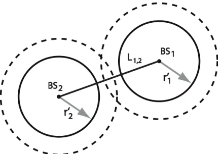
Adopting the path loss model described in Section 3.1 and use the RSS measurements as information to locate MS’s position is cost-effective and easy-implemented. However, not as what most traditional range-free positioning algorithms such fingerprinting tech-nique [15], [16] did to RSS, a simple distance estimation method addressed in Section 3.2 is included in the proposed DALE algorithm to estimate the range measurements and various path loss exponents. In a noise free environment and having knowledge of the true path loss exponent, the signal range measurements can be converted directly from RSS measurements, and they are supposed to intersect in the position of MS. But the distance we obtain might be either extended or shortened due to the existence of the normal-distributed fading effects in the RSS measurements. This could be a severe problem in location algorithms. For example, if two RSS measurements are suffered from positive noises, the converted range measurements will be shorter than they actually are since the noises make the RSS measurements seem to be stronger than they really are, as ri and rj illustrated in Fig. 3.1. But this situation implies that the MS could be located in the

distance of either r1 or r2 apart from BSi or BSj, which dose not make sense physically.

A more reasonable circumstance should be that the two range measurements covers each other. In other words, the summation of any two range measurements is no smaller than the distance between these two BSs, and the relationship can be obtained as

r′_i+ r_j′ ≥ Li,j , ∥BSi− BSj∥ (3.3)

where∥x∥ is the norm of a vector x.

Furthermore, as described in Section 3.2, another problem comes as it require three RSS measurements to perform a two-dimensional linear least square estimation. If each

r’

₁ BS₂ BS₁

L

_1,2

r

2

‘

Figure 3.1: An illustration of outer separate and intersection of two range measurements

BS

₃

r”

BS

₁

BS

₂

V

₁

d

₁

1

two range measurements barely contact with each other as described in (3.3), there are still chances that the three range measurements have no intersection in common, as the real lines illustrated in Fig. 3.2. This implies that the same MS could be located in more than one range intersection and receives RSS measurements simultaneously. Once more, this is impossible. The reasonable case should be that either the three range measurements intersect in the location of MS, or the three range measurements construct an overlapped region. In other words, each two range measurements shall have one or two intersection points. Moreover, it is observed that the necessary condition to form an overlapped region as having three range measurements is that each circle shall cover the nearest vertex formed by other two circles. For example, as illustrated in Fig. 3.2, if the circle 1 with radius r1 is intended to cover the intersection zone formed by circle 2 and

circle 3, it must at least cover the V1, which is the nearest vertex formed by by circle 2

and circle 3. The mathematical constraint shall be as follows

r”2 ≥ d2 =∥BS2− V2∥ (3.4)

where BSi represents the position of the ith BS and Vi represents the position of the ith

vertex formed by the two range measurements other than the ith range measurement. As the aforementioned conditions for three BSs are satisfied, the overlapped region where the MS is supposed to be within could be guaranteed.

Chapter 4

Proposed Diversity-Augmented

Location Estimation Algorithm

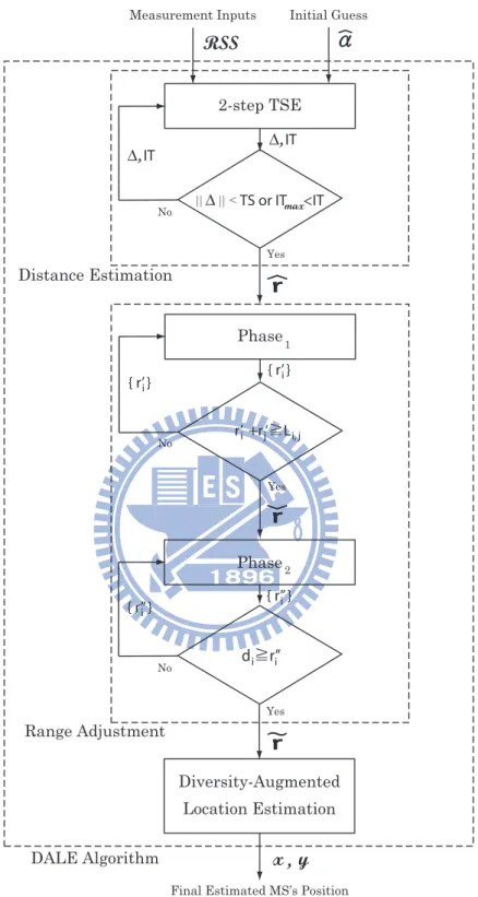
In this chapter, the proposed diversity-augmented location estimation (DALE) algorithm based on RSS measurements and the concepts of linear least square methods as depicted in Section 3.2 will be extended. The algorithm will be introduced in three parts as illustrated by a flow chart in Fig. 4.1. First of all, in Section 4.1, we consider the impact of inaccurate PLE α due to having no information about the channel characteristics of a new environment and thus assigning a rough and empirical initial guess of PLE. This will introduce a serious error during the process of converting RSS into distance due to the given PLE guess. Therefore, the distance estimation (DE) mechanism is proposed to fine-tune PLE and estimate distances with a simple two-step TSE method. And in Section 4.2 we will go through a proposed range adjustment(RA) mechanism. The existence of Gaussian noise in RSS measurements will cause abnormal signal ranges as we discussed in 3.3. We thus propose the RA mechanism to adjust the signal ranges to the reasonable volumes. Section 4.3 comes how we use the idea of virtual base station (VBS) [28] and the ideas of LS methods described in Section 3.2 to acquire some augmented diversity gains on the space domain and obtain a more precise location estimation of the MS’s position.

2-step TSE Measurement Inputs No RSS || || < ∆ TS or IT <IT_max Yes ∆, IT Distance Estimation r ︿ No Yes r’ +r ‘≧L_{i j i, j} DALE Algorithm

Final Estimated MS’s Position

x y, Diversity-Augmented Location Estimation r ∼ No Phase₂ Yes Range Adjustment d ≧r”_{i i} { r’ }_i { r” }_i Phase₁ r ﹀ Initial Guess Ƞ ∆, IT { r’ }_i { r” }_i ︿

4.1

Mechanism of Distance Estimation

In this section, we will introduce the first part of the proposed DALE algorithm, the DE mechanism. As the path loss model mentioned in Chapter 3, we define

Fi , P L′0+ 10α log10ξi

where P L′₀ = P L0+ 20 log fc. The mechanism of the prosed DE scheme is to use TSE to

expand Fi with respect to the two parameters α and ξi as

Fi = Fi|IG1,i +

∂

∂αFi|IG1,i(α− IG1,i) +· · · (4.1)

= Fi|IG2,i +

∂

∂ξFi|IG2,i(ξi− IG2,i) +· · · (4.2)

where α is PLE, ξi represents the distance between MS and the ith BS, and IGi is a set

of initial guess as follows

IGi =    IG1,i IG2,i   

The terms with order equal to or higher than two are relatively trivial and can be ne-glected. One potential drawback of TSE is the requirement of initial guess. The result of TSE would be diverge if we give a set of extremely bad initial guesses. Fortunately, we have simple and reasonable candidates for the initial guesses. Notation IG1,i is a guess of

PLE ˆαi, which will be chosen as a long-term statistics of a space or just giving a

reason-able number after judging the environment. And IG2,i is an initial guess of the distance

between the ith BS and the MS, which will be chosen as the mean of range measurement samples ζi,j, that is, IG2,i = mean(ζi,j)= ˆξi, where i ∈ (1, 3), j ∈ (1, ns), and ns is the

two-step TSE is utilized to estimate ξi after αi iteratively, and iterations is terminated as the

requirements are met.

First of all, we differentiate Fi partially with respect to α

g1,i ,

∂

∂αFi = 10 log10

ˆ

ξi (4.3)

where i represents the index of BSs and j represents the index of the range measurement samples received from BSi. We form an equation as follows

G1∆α = H1 (4.4) where G1 =          g1,i g1,i · g1,i          , H1 =          P Li,1− Fi|ˆαi P Li,2− Fi|ˆαi · P Li,j − Fi|ˆαi         

Solving this equation by the LS method, we can obtain an increment

∆α = (UTU)−1UTV (4.5)

We can update the ˆαi by adding it with ∆α as

ˆ

αi = ˆαi+ ∆α (4.6)

with respect to ξ g2,i , ∂ ∂ξFi = 10 ˆαi ln 10 · 1 ˆ ξi (4.7)

And we form an equations as follows

G2∆ξ = H2 (4.8) where G2 =          g2,i g2,i · g2,i          , H2 =          P Li,1− F_i|ˆξi P Li,2− F_i|ˆξi · P Li,j− Fi|ˆξi         

Solving this equation with LS method, we have an increment ∆ξ

∆ξ = (GT₂G2)−1GT2H2 (4.9)

We can thus update the ˆξi by means of ∆ξ

ˆ

ξi = ˆξi+ ∆ξ (4.10)

The updated IG2,iwill be fed back to conduct the first procedure. We will keep conducting

this two-stage calculation for many rounds. And the iteration will be halted until either condition 1 is met or the conditions 2 and 3 are satisfied

1. maximum iteration times (ITmax)≤ IT

3. ∥∆ξ∥ < TS of ∆ξ

The goal of conducting this DE mechanism is to eliminate the effect of having an inaccurate α, which could cause a severe error during we converting the RSS measurements into distance. After all, the final outcome shall be the updated distance IG2,i, which is

denoted by ˆri and ˆr =

[ ˆ

r1, rˆ2, ˆr3

]T

is obtained as completing the DE mechanism. ˆr is then fed into the following RA mechanism for further processing.

4.2

Mechanism of Range Adjustment

The two-phase method called the RA mechanism is proposed based on the estimations acquired at the DE mechanism and the observations depicted in Section 3.3. In Section 3.3 we have mentioned that it is strange that two range measurements does not have mutual intersection. Hence, it is necessary to examine and adjust the ˆr before conducting location estimations. It is denoted that r′_i is originally equal to ˆri and will be adjust in

the RA mechanism if necessary. Moreover, the parameter Ti,j is assigned as an index to

represent the the geometric relationship between r_i′ and r_j′. Parameter Si,j is defined as

the flag to be assigned to the ith BS with respect to all the other BSj. Therefore, we

check Ti,j and classify them into five cases in phase1 as follows

1. If two range measurements r′_i and r′_j are too small to reach each other, Ti,j is defined

as ”outer separation”, and assigning k1 flags to ri′ and k1 flags to r′j.

2. If two range measurements r_i′ and r′_j intersect each other in two points, Ti,j is defined

as ”intersection”, and assigning 0 flag to both r′_i and r′_j.

3. If the range measurement r_i′ contains range measurement r_j′, Ti,j is defined as

4. If the range measurement r_i′ is contained by range measurement r_j′, Ti,j is defined

as ”containing”, and assigning k1 flags to r′i and -k1 flags to rj′.

5. If two range measurements r′_i and r′_j intersect each other in one point, Ti,j is defined

as ”tangency”, and assigning 0 flag to both r_i′ and r_j′.

After all, we sum up the flags of ith BS with respect to the jth BS as follows

Si =

∑

j,i̸=j

Si,j (4.11)

Multiplying Siwith the ith link’s measurement standard deviation σmi, and we can obtain

the adjustment to update r_i′. That is, r′_i = r_i′+ ∆r_i′, where ∆r_i′ = σmiSi. In phase1 we will

keep this iterative calculation until each two ranges have intersect in common or at least tangent each other. The mechanism of RA’s phase1 is illustrated by the pseudo code in

Algorithm 1.

After phase1’s adjustment, the final output should be ˇr, where ˇr =

[

r₁′, r′₂, r′₃

]T

and it will be fed into phase2 for the sake of the observations in Section 3.3. There might

still have chances that each two ranges intersect with each other but three ranges have no intersection region in common, as described in Section 3.3. Thus we propose the second phase to prevent it. In phase2 we are going to propose another process to make sure

the 3 ranges will intersect others or even intersect in exactly one point. Any two circles intersect with each other will result in at least one vertex. First of all, we calculate the Vp,

one of the intersection point of r”i and r”j which is the one closet to BSp, where i ̸= j,

i̸= p and j ̸= p and i, j, p = 1, 2, and 3. As constraint (3.4) we discussed in Section 3.3

that guarantees the existence of common overlapped region. r”p ≥ dp =∥BSp− Vp∥

If the constrain is not satisfied in the pth link, we will add ∆r”i to r”i, that is, r”i = r”i+

∆r”i, where ∆r”i = k2σi, i̸= p. We will keep doing this mechanism until constraint (3.4)

is satisfied for all p. The final output of phase2will be ˜r, where ˜r =

[

r”1, r”2, r”3

]T

Algorithm 1: Range Adjustment P hase1

Ti,j: Relation between BSi and BSj

Li,j: The distance between BSi and BSj

r_i′: The ith range measurement

σmi: The standard deviation of measurements in the ith link

Si,j: The flag assigned

kp: The step size of adjustment per round in phasep

begin

while (Ti,j ̸=intersection) & (Ti,j ̸=tangency) do

forall the N odei and N odej, i̸=j do

if r_i′+ r′_j < Li,j then

Ti,j = outerseparation;

Si,j = k1;

Sj,i= k1;

else if r_i′+ r′_j > Li,j then

if r_i′+ Li,j < rj′ then

Ti,j = contained;

Si,j = k1;

Sj,i=−k1;

else if r_i′ > r′_j+ Li,j then

Ti,j = containing; Si,j =−k1; Sj,i= k1; else Ti,j = intersection; Si,j = 0; Sj,i= 0; end

else if r_i′+ r′_j = Li,j then

Ti,j = tangency;

Si,j = 0;

Sj,i= 0;

end end

forall the N odei, N odej, i̸=j do

r_i′ = r_i′+ σmi ∑ jSi,j; end end end

The mechanism of RA’s phase2 is illustrated by the pseudo code in Algorithm 2.

Algorithm 2: Range Adjustment P hase2

dp: Distance between BSp and Vp

begin

while dp > Rp do

forall the N odep do

r”i= r”i+ k2σmi;

r”j = r”j+ k2σmj;

end end end

4.3

Diversity-Augmented Location Estimation

As illustrated in Fig. 4.2, three BSs associated with the three range measurements are utilized for the location estimation of the MS. The overlap region (i.e. confined by the arcs V1V2, V1V3, and V2V3) is formed by the mechanism of RA as we described in Section

4.2. Since the objective of the proposed DA location estimation is to expand the spatial diversity, the following definitions and the associated constraint cost function are defined: Definition 4.1 (Virtual Distance). The parameter γi (for i = 1 to 3) is defined as the

ith virtual distance between the MS’s position and Vi as

γi =∥x − Vi∥ (4.12)

where x is the MS’s location; Vp represents the intersecting points around the overlap

region, i.e. V1 = (xv1, yv1), V2 = (xv2, yv2), and V3 = (xv3, yv3) are the corresponding

coordinates of the points V1, V2, and V3.

It is noted that the value of γi varies as the three coordinates V1, V2, and V3 are

BS

₃

r

₁

BS

₂

BS

₁

r

3

∼

r

₁

∼

r

₃

∼

r

₂

r

₂

ȴ

ȧ

V

₂

x

_e

V

₃

V

1

︿ ︿ ︿

Ȣ

_e

3

Figure 4.2: An illustration of range measurements after RA mechanism and the result of

BS

₂

BS

₁

BS

₃

V₁ ∼

r

₁

∼

r

₃

∼

r

₂

V₂ V₃

x

_e

Ȣe₁ Ȣe₂ Ȣe₃

Figure 4.3: An illustration of range adjustment and the projection of error variance

triangular area V1V2V3 in order to fulfill the constraints from the geometric layout. The

corresponding ith expected virtual distance γei can be defined as follows

Definition 4.2 (Expected Virtual Distance). The ith expected virtual distance γei is

defined as

γei =∥xe− Vi∥ = γi+ nγ_ei (4.13)

where xe is the expected position of the MS, and nγ_ei denotes the error induced by the

computed deviation between γei and γi.

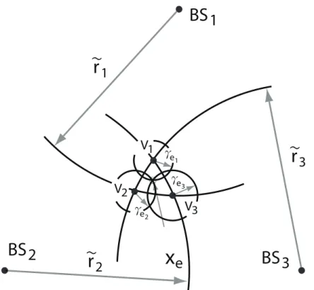
The major objective by adapting the geometric assistance in the DA location estima-tion is to create three addiestima-tional virtual BS as if they were transmitting signals to MS, which can be used to improve the performance of following LS method. We view the points {Vi} illustrate in Fig. 4.2 as VBSs, and the set of virtual distances γe as range

measurements, where γe = [γe1, γe2, γe3]. Moreover, the expected position of MS, x, can

be viewed as a virtual mobile station (VMS) as illustrated in Fig. 4.3. We can thus form three additional equations similar to those in the real world. The selection of the VMS’s position xe is obtained by weighting the points {Vi} with the signal variations from the

theree range measurements. The coordinates of xe = (xe, ye) are chosen with different

weights (w1, w2, w3) w.r.t. the V1, V2, and V3 points of the triangle as

xe = n

∑

k=1

wkVk (4.14)

where n = 3 in this case, and Vk are the vertexes as illustrated in Fig. 4.3 with

coor-dinates as (xvk,yvk). The weighting coefficients wk are defined based on the effects from

both the standard deviations and the relative distance w.r.t. the corresponding range measurements, which can be obtained in the same way as [27]. Based on an appropriate selection of the weighting coefficients, the VMS’s position xe is obtained. The ith expected

virtual distance γei can therefore be computed from equation (4.13), and the proposed

DA location estimation can be formulated by solving the TSLS problem as we described in Section 3.2 with the additional geometric assistance, which are originated from the virtual concept among the overlapped region. The solution is obtained by minimizing both the errors coming from the output of RA (that is, ˜r) and the deviations between the expected virtual distances and the virtual distances (as shown in equation (4.12)). By rearranging and combining ˜ri and (4.13) in the matrix format, the following equation can

be obtained:

where ˆz1 = [ x(1) y(1) λ ]T and H1 =    H 3×3 ˜ r H3_γ×3    =                 −2x1 −2y1 1 −2x2 −2y2 1 −2x3 −2y3 1 −2xv1 −2yv1 1 −2xv2 −2yv2 1 −2xv3 −2yv3 1                 (4.16) J1 =    J 3×1 ˜ r J3_γ×1    =                 ˜ r₁2− κr˜1 ˜ r₂2− κr˜2 ˜ r₃2− κr˜3 γ2 e1 − κγe1 γ2 e2 − κγe2 γ2 e3 − κγe3                 (4.17)

The corresponding coefficients are given by

λ = x2₍₁₎+ y₁2

κℓ= x2ℓ + y

2

ℓ for ℓ = 1, 2, 3

The expected virtual distances γei (as shown in equation (4.17)) are served as the virtual

measurements, comparing with those true measurements rℓ, for ℓ = 1, 2, and 3. The

noise component of ˜n in ˜r is consisted of nm and nRA, where nm are the noises of range

measurements, and nRA is the noise that is introduced during the RA mechanism. Since

the coordinates of V1, V2, and V3 are obtainable after the ˜r are acquired, we depict the

example, as illustrated in Fig. 4.2, the noise of γe3 shall be nγ_e3 = ˜n1cos θ + ˜n2cos φ. It

is noted that θ is the angle between γe3 and ˜r1, while φ is the angle between γe3 and ˜r2.

The measurement noise matrix ψ in (4.15) can be obtained as

ψ1 = B1n + n2

where

B = diag{˜r1, r˜2, r˜3, γe1, γe2 γe3}

n =[n˜1, n˜2, n˜3, nγ_e1, nγ_e2, nγ_e3

]T

Based on the DA location estimation scheme, an intermediate estimate ˆz1 after the first

step can be obtained as

ˆ z = [ x(1) y(1) λ ]T = (HT₁Ψ−1₁ H1)−1HT1Ψ−11 J1 (4.18)

where (x(1), y(1)) is denoted as the intermediate location estimation of the MS after the

first step of the algorithm, λ = x2₍₁₎+ y₍₁₎2 . The weighting matrix Ψ1 is obtained as

Ψ1 = E[ψ1ψ1T] = 4B1QB1

It is noted that Ψ1 is acquired by neglecting the second term of (4.18). The matrix Q

becomes Q = diag { ˜ σ₁2, σ˜₂2, ˜σ2₃, σ2_γ e1, σ 2 γ_e2, σ 2 γ_e3 }

It can be observed that Q represents the covariance matrix for both the TOA measure-ments and the expected virtual distances, where σγ_ei corresponds to the standard deviation

of γei. For the convenience of analysis, we assume that the noise of range measurement

is independent of the noise of RA mechanism, that is, nmi ⊥ nRAi. And thus ˜σ

2

i can be

written as the sum of σ_m2_i and σ_RA2 _i, where σ_m2_i is the noise variance of the range

measure-ment of the ith channel, and σ2

RAi is the variance of range measurement’s modification

due to the RA mechanism as we depicted in Section 4.2. The detailed derivation of σ2

RAi

will be described as follows.

From equations (3.1) and (3.2), we have

ˆ ri = exp [ (ln 10 10α)Li ] = exp [ (ln 10 10α)(10α( ln ξi ln 10) + ni) ] = ξiexp [ (ln 10 10α)ni ] (4.19) where Li , P Li− P L′0 = 10α( ln ξi ln 10) + ni

We define βi = exp(ln 10_10αni) and taking nature logarithm of it to have ln βi = ln 10_10αni ∼

N (0, σ2

ln βi), where σln βi =

ln 10

10αni. The statistical characteristics and probability density

function (PDF) of the log-normal distributed variable βi shall be

µβi , E[βi] = exp( 1 2σ 2 mi) σ_β2_i , V ar[βi] = exp(σln β2 i) ( exp(σ_{ln β}2 _i)− 1) fβ(βi) = 1 βi √ 2πσln βi exp [ −1 2( ln βi σln βi )2 ] , βi > 0

From equation (4.19), we have ˆri = ξiβi. It is also log-normal distribution. Taking

nature logarithm from it and we will have ln ˆri = ln ξi+ln βi ∼ N (µln ˆri, σ

2

ln ˆri), where µln ˆri

= ln ξiand σln ˆ2 ri = σ

2

βi. We can thus have ˆri’s mean µˆri , E[ˆri] = exp(ln ξi+

1 2σ

2

ln ˆri) = ξiµβi

and variance σ_m2_i , V ar[ˆri] = exp(ln ξi+ 1₂σ2ln ˆri)(exp(σ

2

ln ˆri)− 1) = (ξiσβi)

2_.

of range measurement as ˆni , ˆri− ξi = ξiνi, where νi = βi− 1, and νi ∈ (−1, +∞). νi is a

random variable with shifted log-normal distribution. µνi , E[νi] = E[βi− 1] = µβi− 1,

and σ_ν2_i , V [νi] = V [βi] = (σβi)

2_{. Since ˆn}

i = ξiνi, we can know that µˆni , E[ξiνi] =

ξi(µβi − 1) = µrˆi − ξi and σnˆi , V ar[ξiνi] = (ξiσβi)

2 _{= σ}2

mi. Here nˆri is also a shifted

log-normal random variable with support (−ξi, +∞). We can thus derive νi’s PDF from fβ(βi) as follows. fV(νi) = fβ(βi)  dβi dνi  ,βi > 0 = 1 (νi+ 1) √ 2πσln βi exp [ −1 2( ln(νi+ 1) σln βi )2 ] , νi > 1 (4.20)

Moreover, we derive ˆni’s PDF by means of νi’s.

f_Nˆ(νi) = fV( ˆ ni ξi )dνi dˆni  , ˆni >−ξi = 1 (nˆi ξi + 1) √ 2πσln βi exp [ −1 2( ln(nˆi ξi + 1) σln βi )2 ] 1 ξi = 1 (ˆni+ ξi) √ 2πσln βi exp [ −1 2( ln(ˆni ξi + 1) σln βi )2 ] = 1 ˆ ri √ 2πσln βi exp [ −1 2( ln(rˆi ξi) σln βi )2 ] , ˆri > 0 = 1 ˆ ri √ 2πσln βi exp [ −1 2( ln(ˆri)− ln(ξi) σln βi )2 ] = f_Rˆ(ˆri) (4.21)

We would like to know the errors that happened between range measurements as we consider the rationality of the geometric relations as described in Section 3.3. Moreover,

we define ηi,j = k ⌈ ˆ ni+ ˆnj k(σmi+ σmj) ⌉ ,−ξi− ξj < ˆni + ˆnj

as the total number of adjustment times for both the range measurements ˆri and ˆrj,

i, j ∈ (1, 3), i ̸= j, and k is the number of flag we assign to each range measurement per

iteration round.

According to the properties of ceiling function,

k( ⌈ ˆ ni k(σmi + σmj) ⌉ + ⌈ ˆ nj k(σmi+ σmj) ⌉ )− 1 < ηi,j < k( ⌈ ˆ ni k(σmi + σmj) ⌉ + ⌈ ˆ nj k(σmi+ σmj) ⌉ ) (4.22)

Assume {ni}i=1,2,...,N are I.I.D., then {ˆni}i=1,2,...,N are supposed to be independent, and

{ˆni}i=1,2,...,N shall also be independent. That is, fN(ˆni, ˆnj) = f_Nˆ(ˆni)fNRA(ˆnj). Since

since ηi,j is bounded, from equation (4.22) we know that σ2ηi,j = σ

2 Yi + σ 2 Yj, where Yi , ⌈ ˆ ni k(σ_mi+σ_mj) ⌉ , −ξi k(σ_ri+σ_rj) < Yi,∀Yi ∈ Z. To obtain σ 2 Yi, we first derive Yi’s CDF as follows FY(yi) = P (Yi ≤ yi) = P ( ⌈ ˆ ni k(σmi + σmj) ⌉ ≤ yi) = P ( ˆ ni k(σmi+ σmj) ≤ yi) (N ote : x≤ n ⇔ ⌈x⌉ ≤ n) = P (ˆni ≤ k(σmi+ σmj)yi) = ∫ k(σ_mi+σ_mj)yi −ξi 1 (ˆni+ ξi) √ 2πσln βi exp [ −1 2( ln(ˆni+ ξi)− ln ξi σln βi )2 ] dˆn = ∫ ln(k(σmi +σmj )yi+ξi)−lnξi σln β_i −∞ 1 √ 2πexp [ −1 2g 2 ] dg, g , ln(ˆni+ ξi)− ln ξi σln βi (4.23) = Φ ( ln(k(σmi+ σmj)yi+ ξi)− lnξi σln βi ) ,− ξi k(σmi+ σmj) < yi, yi ∈ Z

rule to derive its probability mass function (PMF) PY(yi) as follows. PY(yi) = dFY(h(yi)) dh dh dy, h(yi), ln(k(σmi+ σmj)yi+ ξi) + ln ξi σln βi from equation (4.23) FY(h(yi)) dh = d dh ∫ h(yi) −∞ 1 √ 2πexp [ −1 2g 2 ] dg = √1 2πexp [ −1 2( ln(k(σmi+ σmj)yi+ ξi) + lnξi σln βi )2 ] dh dy = 1 σln βi · 1 k(σmi+ σmj)yi+ ξi · k(σmi+ σmj) ⇒ PY(yi) = 1 √ 2πexp [ −1 2( ln(k(σmi + σmj)yi+ ξi) + ln ξi σln βi )2 ] · k(σmi + σmj) σln βi(k(σmi+ σmj)yi+ ξi) = k(σmi+ σmj)· 1 (k(σmi+ σmj)yi+ ξi) √ 2πσln βi exp [ −1 2( ln(k(σmi + σmj)yi+ ξi) + lnξi σln βi )2 ]

Since it is hard to find the variance σ_Y2_i from the complicate PMF, we acquire it in the

computational way as ∑1000_y

i=⌈k(σ_mi+σ_mj)⌉PY(yi). After conducting all the computation of

σ2

Yi and σ

2

Yj, we can thus acquire σ

2 ηi,j = k 2_σ2 Yi+ k 2_σ2 Yj. The σ 2

RAi shall be the summation

of all the σ2

ηi,j multiplies σ

2

i where i̸= j, that is, σ2RAi = σ

2 i ∑ i,i̸=jσ 2 ηi,j as nRAi is defined by σi ∑ jηi,j.

To extract the relationships of x(1), y(1) and λ, second step of the DA location

estima-tion scheme can be obtained as [19]:

ˆ x = [ ˆ x yˆ ]T =[(HT₂Ψ−1₂ H2)−1HT2Ψ−12 J2 ]1/2 (4.24)

where H2 =    1 0 1 0 1 1    T J2 = [ ˆ x2 i yˆi2 βˆ ]T Ψ2 = E[ψ2ψT2] = 4 B2 cov(ˆz)B2 = 4 B2 (HT1Ψ−11 H1)−1 B2 (4.25) B2 = diag{ˆxi, yˆi, 1/2}

The final output of the proposed DALE algorithm will be (ˆx, ˆy) after solving the second

step of DA location estimation as described in equation (4.24) and choosing the one that is nearest to ˆz1.

Chapter 5

Performance Evaluation

In this chapter, simulations are conducted to show the effectiveness of the proposed DALE algorithms under different network topologies and MS’s positions. The noise model of RSS measurements will be the same as we described in section 3.1. The slow fading effect will be Gaussian-distributed with mean µ equal to zero and standard deviation σ in the range from 3-6 dB. IEEE 802.11a [29] defined the operation frequency at 5.0GHz, while 2.4GHz in IEEE 802.11b [30]. Nowadays many wireless fidelity (Wi-Fi) devices are mainly operating at frequency band around 2.4-2.5 GHz, so we roughly choose the carrier frequency fc as 2.45 GHz. The remaining common simulation parameters are

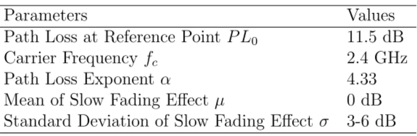
referred to the 3GPP TR 36.814 report [24] as we mentioned in section 3.1 and are listed in Table 5.1. We will evaluate the effectiveness of the proposed DE mechanism first.

Table 5.1: Simulation parameters

Parameters Values

Path Loss at Reference Point P L0 11.5 dB

Carrier Frequency fc 2.4 GHz

Path Loss Exponent α 4.33

Mean of Slow Fading Effect µ 0 dB

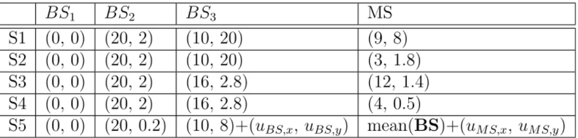
Table 5.2: Deployment of BSs and MS BS1 BS2 BS3 MS S1 (0, 0) (20, 2) (10, 20) (9, 8) S2 (0, 0) (20, 2) (10, 20) (3, 1.8) S3 (0, 0) (20, 2) (16, 2.8) (12, 1.4) S4 (0, 0) (20, 2) (16, 2.8) (4, 0.5)

S5 (0, 0) (20, 0.2) (10, 8)+(uBS,x, uBS,y) mean(BS)+(uM S,x, uM S,y)

Then the performance comparison between the proposed DALE algorithm with the other existing location estimation methods are conducted in three types of network layouts. First, we arrange the three BSs in the layout to be close to a regular triangle. Secondly we deploy the three BSs to be like an irregular triangle. In the third topology, we put the three BSs randomly in the space, trying to obtain an arbitrary triangle as evaluating the performance in random cases. Therefore, 5 scenarios are taken into account and the related deployment parameters is given in the Table 5.2, where uBS,x, uBS,y ∼ U(−6, 6),

uM S,x, uM S,y ∼ U(−10, 10) with constraints that the MS must lie in the triangle formed

by BSs and the distance between MS and each BS must larger than 3 meters according to the path loss model in [24]. Mean(BS) represents the gravity center (GC) of BSs’ layout. For the convenience of evaluation, we define PLE’s true value as ˆα and the PLE

estimation result of the proposed DE mechanism as ˆα. The PLE estimation error αe is

defined as

αe = ˆα− α

For the convenience of evaluation, we define MS’s true position as x = (x, y) and the estimation output of location algorithms as ˆx = (ˆx, ˆy). The location estimation error Le

is defined as

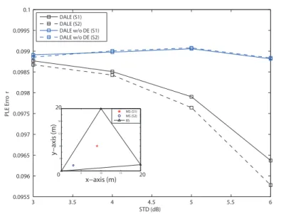
3 3.5 4 4.5 5 5.5 6 0.0955 0.096 0.0965 0.097 0.0975 0.098 0.0985 0.099 0.0995 0.1 STD (dB) PLE Erro r DALE (S1) DALE (S2) DALE w/o DE (S1) DALE w/o DE (S2) 5 10 15 20 0 4 8 12 16 20 x−axis (m) y− axis (m) MS (S1) MS (S2) BS

Figure 5.1: The relationship between PLE estimation error and noise standard deviation in a

regular triangle

The mean square error (MSE) is thus defined as

M SE = mean(∥ˆx − x∥2) (5.2)

where mean(x) is the sample mean of the elements in the vector x. The value of PLE initial guess ˆα is 4.23, which has a bias of 0.1 from the long-term mean value of true PLE α

defined in Table 5.1. A random bias uniformly-distributed with [-0.05, 0.05] is appended to the true PLE α to represent the randomness of the real PLE of each propagation channel. The performance is evaluated with 30000 independent trials. The initial guess will be chosen as an arbitrary point with 1 meter from the MS’s true position for any algorithm that requires that.

The objective of the DE mechanism is to estimate the PLE and the distance with RSS measurements and the estimation performance is investigated under different scenarios defined in Table 5.2. The initial guesses of the PLE and distance for the TSE-based DE mechanism are obtained as described in Section 4.1. Fig. 5.1 and Fig. 5.2 are the

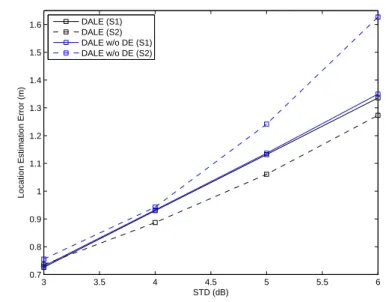
3 3.5 4 4.5 5 5.5 6 0.7 0.8 0.9 1 1.1 1.2 1.3 1.4 1.5 1.6 STD (dB)

Location Estimation Error (m)

DALE (S1) DALE (S2) DALE w/o DE (S1) DALE w/o DE (S2)

Figure 5.2: The relationship between location estimation error and noise standard deviation

in a regular triangle

estimation errors of PLE and distance in scenarios S1 and S2 with respect to different noise standard deviations. It is noted that the scenario S1 represents a network topology with the BSs locate as a regular triangle whose center the MS lies at, while the scenario S2 has the MS locates somewhere apart from the center of the network. We evaluate the performance of our proposed DALE algorithm with the schemes of DALE without the DE mechanism (DALE w/o DE) to see whether the DALE algorithm have any improve by performing the DE mechanism. In Fig. 5.1 we can see that for those schemes with DE mechanism, that is, DALE (S1) and DALE (S2), have less PLE estimation error, while the schemes without DE mechanism have a constant bias because they do not have any mechanism to estimate the PLE. On the other hand, in Fig. 5.2, we can make an intuitive conclusion that since DALE algorithm has the correction of PLE and thus it has less location estimation error in both scenario S1 and S2. Moreover, we notice that the PLE estimation in S2 is better than that in S2. This makes the location estimation error in S2 is less than that in S1. We thus make a brief conclusion that the better PLE estimation one have, the better location estimation results can be obtained.

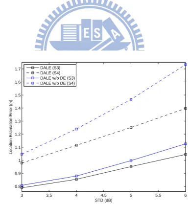
3 3.5 4 4.5 5 5.5 6 0.0955 0.096 0.0965 0.097 0.0975 0.098 0.0985 0.099 0.0995 0.1 STD (dB) PLE Error DALE (S3) DALE (S4) DALE w/o DE (S3) DALE w/o DE (S4) 5 10 15 20 0 1 2 x−axis (m) y−axis (m) MS in (S3) MS in (S4) BS 3

Figure 5.3: The relationship between PLE estimation error and noise standard deviation in

an irregular triangle 3 3.5 4 4.5 5 5.5 6 0.8 0.9 1 1.1 1.2 1.3 1.4 1.5 1.6 1.7 STD (dB)

Location Estimation Error (m)

DALE (S3) DALE (S4) DALE w/o DE (S3) DALE w/o DE (S4)

Figure 5.4: The relationship between location estimation error and noise standard deviation

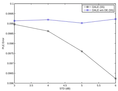
3 3.5 4 4.5 5 5.5 6 0.096 0.0965 0.097 0.0975 0.098 0.0985 0.099 0.0995 0.1 STD (dB) PLE Error DALE (S5) DALE w/o DE (S5)

Figure 5.5: The relationship between PLE estimation error and noise standard deviation in

an arbitrary triangle

The performance of the DE mechanism in the scenarios S3 and S4 is studied in Fig. 5.3 and Fig. 5.4. In Fig. 5.3 we can discover that DALE (S3) and DALE (S4) have less PLE estimation error than the scheme without DE mechanism which has a constant bias. Observing from Fig. 5.4 we notice again that the one with better PLE estimation will has less location estimation error in both S3 and S4. Since the PLE estimation in S4 is better than that in S3, it makes better location estimation in S4 than in S3. Therefore, it is revealed again that better PLE estimation is coupled with better distance estimation. In the scenario S5, a random network topology is applied as addressed in Table 5.1. According to the path loss model in TR 36.814 [24], the distance between the MS and any BS should be larger than 3 meters. The Fig. 5.3 and Fig. 5.4 represent the estimation performance of the DE mechanism in S5. The DALE has the PLE with less bias, thus its location estimation error is less than the DALE without DE scheme. By the general case, we can confirm the effectiveness of the DE mechanism can be ensured. The location errors of the DALE algorithm and many other methods are also evaluated in the scenarios mentioned above. The performance of our proposed DALE algorithm

3 3.5 4 4.5 5 5.5 6 0.95 1 1.05 1.1 1.15 1.2 1.25 1.3 STD (dB)

Location Estimation Error (m)

DALE (S5) DALE w/o DE (S5)

Figure 5.6: The relationship between location estimation error and noise standard deviation

in an arbitrary triangle 0 0.5 1 1.5 2 2.5 3 0 0.1 0.2 0.3 0.4 0.5 0.6 0.7 0.8 0.9 1

Location Estimation Error (m)

CDF (% ) DALE (S1) DALE (S2) DALE w/o DE (S1) DALE w/o DE (S2) DALE w/o W (S1) DALE w/o W (S2) TSLS (S1) TSLS (S2) TSE (S1) TSE (S2) 5 10 15 20 0 4 8 12 16 20 x−axis (m) y−axis (m) MS (S1) MS (S2) BS

Figure 5.7: The comparison of location estimation error under the fading noise with 4 dB

is compared with the schemes of DALE without the DE mechanism (DALE w/o DE), DALE without the design of weighting (DALE w/o W), TSLS algorithm [19] as well as TSE algorithm [18]. It is noted that the proposed DALE in scenario 1 is close to other algorithms, especially the DALE without DE scheme. This is due to the perfect layout of BSs that reduces the effect of noise. However, DALE (S1) is still the one with the best performance. In scenario S2, the MS moves toward one corner of the regular triangle, making the MS become closer to one of the MS than scenario S1. This increase the chance of having bad performance for all the algorithms because the shortest distance between MS and BSs become very short. Any noise with extreme value could cause a significant ratio of change in the shortest path, which could lead to a severe error in the calculation results. However, we can still discover that our proposed DALE (S2) have the best performance in Fig. 5.7. Without any weighting, the DALE w/o W scheme could be even worse than the TSLS and TSE that have taken noise STD as weighting design. For our proposed DALE with moderate weighting, it turns into the best one. Moreover, it is not hard to discover that the gain of DE is tiny in these two scenario. This could be not extremely bad layout that makes the gain of RA mechanism to be tiny.

In equations of (5.1) and (5.2), we think that the location estimation error and MSE has a kind of positive correlation. For the clearness of illustration, we eliminates the DALE w/o DE and DALE w/o W schemes in our MSE Figures since they do not have better performance than DALE in the CDF of location estimation error. In other words, we will evaluate the performance of our proposed DALE algorithm with TSLS algorithm, and TSE algorithm. In Fig. 5.8, we compare the MSE of the algorithms we just mentioned. Similar to what we saw in Fig. 5.7, in scenario S1 all the algorithms have the performance closed to each other, while in S2, the bad layout formed by the BSs make all the algorithms to have worse estimation results.

3 3.5 4 4.5 5 5.5 6 100 101 STD (dB) MSE (m 2) DALE (S1) DALE (S2) TSLS (S1) TSLS (S2) TSE (S1) TSE (S2)

Figure 5.8: The comparison of mean squared error in the scenarios S1 and S2

0 0.5 1 1.5 2 2.5 3 3.5 0 0.1 0.2 0.3 0.4 0.5 0.6 0.7 0.8 0.9 1

Location Estimation Error (m)

CDF (% ) DALE (S3) DALE (S4) DALE w/o DE (S3) DALE w/o DE (S4) DALE w/o W (S3) DALE w/o W (S4) TSLS (S3) TSLS (S4) TSE (S3) TSE (S4) 5 10 15 20 0 1 2 x−axis (m) y−axis (m) MS in (S3) MS in (S4) BS 3

Figure 5.9: The comparison of location estimation error under the fading noise with 4 dB