Source Model for Transform Video Coder and
Its Application—Part I: Fundamental Theory
Hsueh-Ming Hang,
Senior Member, IEEE, and Jiann-Jone Chen
Abstract—A source model describing the relationship between
bits, distortion, and quantization step sizes of a large class of block-transform video coders is proposed. This model is initially derived from the rate-distortion theory and then modified to match the practical coders and real image data. The realistic constraints such as quantizer dead-zone and threshold coefficient selection are included in our formulation. The most attractive feature of this model is its simplicity in its final form. It enables us to predict the bits needed to encode a picture at a given distortion or to predict the quantization step size at a given bit rate. There are two aspects of our contribution: one, we extend the existing results of rate-distortion theory to the practical video coders, and two, the nonideal factors in real signals and systems are identified, and their mathematical expressions are derived from empirical data. One application of this model, as shown in the second part of this paper, is the buffer/quantizer control on a CCITTP 2 64 k coder with the advantage that the picture quality is nearly constant over the entire picture sequence.
Index Terms— Image coding, rate distortion theory, source
coding.
I. INTRODUCTION
T
RANSFORM coding is a very popular technique in image compression. It is one of the key components in the international video communication standards [1]–[3]. Often, the communication channel poses constraints on the bit rate it can accept, the video coder bit rate control or output buffer control becomes one of the critical problems in designing a video compression system. In order to predict the effect (output bit rate) due to the adjustment of coding parameters, it is very desirable to be able to construct a source model that can estimate the bits produced by a video coder for a chosen set of coding parameters.There are two approaches in constructing such a source model: 1) the analytic approach that constructs a mathematical description of a coder by analyzing the structure and behavior of every component in the coder and 2) the empirical approach that derives the input/output relationship of a coder based on the observed data. Although the analytic model of a simple quantizer already existed for a long time [4]–[6], the complete analysis of a standard transform coder has not, to
Manuscript received May 27, 1995; revised June 1, 1996. This paper was recommended by Associate Editor W. Li. This work was supported in part by the National Science Council of R.O.C., Taiwan, under Grant NSC82-0404-E009-176.
The authors are with the Department of Electric Engineering, National Chiao Tung University, Hsinchu, Taiwan, 300, R.O.C.
Publisher Item Identifier S 1051-8215(97)01140-3.
our knowledge, been fully explored. An attempt is made by Hang et al. [7], but it does not contain rigorous theoretical justification. On the other hand, several studies on source modeling [8], [9] based on the empirical data have been reported. Although the empirical approach is rather useful in practice, it does not provide us with insights on the principles of video coder operations and the amount of information contained in an image sequence. In addition, because it is derived from the training data, one may worry about its robustness—its performance on the unknown data because these data may be rather different from the training data statistically.
Our approach in this paper belongs to the analytic approach category. We decompose both the coding system and im-age signal into components of known mathematical models and then combine them together to form a complete de-scription. The theoretical foundation of this approach is the rate-distortion theory. A few elements in our model already exist in the literature. Our contribution is two fold. One, we combine and extend the existing results to the standard-type video coders, and two, the nonideal factors in real signals and systems are incorporated as adjustable parameters to compensate their bias effects on the ideal model. The goal is to build a general source coding model that can be used to predict the coder behavior by taking simple and basic measures of signals such as variances.
This paper is organized as follows. We first briefly review the rate distortion theory of Gaussian signals and uniform quantizers that are relevant to our coder source model. In Sections III and IV, we derive the source model by putting the known elements together with our own extensions. The parameters in our model, which are originally derived from theory, are adjusted to match real pictures and the standard coding algorithms in practical applications. The impact of the nonideal factors in picture and practical coders on our source model are discussed in Sections V-A and V-B. The numerical values of model parameters computed based on the compressed image data are described in Section V-C. Section VI summarizes the results presented in this paper.
II. RATE-DISTORTION MODEL OFQUANTIZER In this section, the one-dimensional (1-D) discrete signal properties relevant to this paper are briefly reviewed, and then these properties are extended to the two-dimensional (2-D) signals. Extensions are often straightforward under the assumptions we made on the 2-D signals.
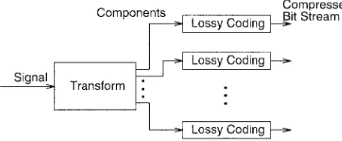
Fig. 1. Signal decomposition using transform.
A. Stationary Gaussian Process
The following results known in information theory are the bases of our future discussions. First, if a (composite) signal can be decomposed into two or more independent components, then its (total) rate-distortion function can be derived directly from the rate distortion functions of the individual compo-nents. In theory, there is no loss of compression efficiency in decomposing a composite signal into simpler components and then compressing each component independently [6].
Second, the rate distortion functions of a few independent
identically distributed (i.i.d.) sources are known such as the
i.i.d. Gaussian sequence. Based on the proposition stated in the above, the rate-distortion functions of signals with memory can be derived by decomposing these signals into independent components with known rate-distortion functions. An example is the stationary Gaussian process. We can apply Fourier transform to it and transformed frequency components are i.i.d. Gaussian sequences. This procedure also suggests a way for compression. That is, an optimal procedure for compressing stationary random processes is to transform a composite signal into independent components and then apply the ordinary data compression techniques to each component separately [10]. A pictorial illustration of this concept is shown in Fig. 1.
The well-known rate distortion function of a discrete station-ary Gaussian process under the mean square distortion criterion is given as [6], [10]
(1) and
(2)
where and is the power spectrum density function
of , and
Region and
Region .
An interpretation of the above formula is that is the minimum bit necessary to achieve an average distortion by an ideal coder of possibly unbounded complexity and time delay. Similarly, is the minimum average distortion that
can possibly be achieved at bit rate . In (1) and (2), is a dummy parameter whose value is decided by a selected or value. The above formulas suggest that to achieve the optimum coding performance, the frequency components of power less than should be discarded and an amount of distortion should be imposed on every one of the retained frequency components.
In reality, we cannot use infinite length transforms to decompose a signal sequence. A typical approach is to partition a signal sequence into nonoverlapped blocks and perform block transformation on each data block separately. There are two problems associated with this approach. One is the correlation among the neighboring blocks, which can be significant for the low frequency components. A part of this correlation can be reduced by applying another layer of correlation reduction techniques on the low frequency components of nearby blocks. The other problem is the power spectrum used in (1) and (2). Practically, the signal power spectrum has to be estimated from data samples. A simple and popular spectrum estimation method is the periodogram that computes the spectrum based on the weighted average of the Fourier transforms of nonoverlapped data blocks [11]. This method is consistent with the finite-size transform we use in data compression if we view the block transform components as the discrete approximation of the ideal continuous power spectrum. Assuming a uniform sampling grid in the frequency domain, (1) and (2) can thus be approximated by the following discrete versions:
(3) and
(4)
where is the number of samples in a data block, and . This is exactly the system represented by Fig. 1 with components.
One may note that (3) can be rewritten as
(5)
where . An interesting property of the above equa-tion is that the exponential funcequa-tion of bit rate is proporequa-tional to the product of the variances of the signal components rather than the sum of variances.
A case of interest is that at low distortion when (or is empty), (4) becomes . And thus, (5) becomes
or
(7) where
(8)
Essentially, we are approximating a joint Gaussian source by multiple i.i.d. Gaussian sources. If the approximation errors can be viewed as white noise, because the power of high frequency components is much lower than that of low frequency components for typical images, the SNR values of high frequency components are smaller. According to (7) and (8), the total distortion is proportional to the product of component power. Hence, a 50% error in one component would translate to 50% total error. Therefore, we should weight the higher frequency components less in the process of selecting quantization parameters in coding. In addition, the unequal frequency weighting also matches the uneven human visual sensitivity.
There are two frequency weighting approaches. One is using the uneven frequency-dependent weights in assigning bits to each frequency component in (3). The other is using uneven weights in computing the total distortion in (4). A special case of the former, frequency-weighted bit allocation, is discussed in Section II-C. A study of the latter, the frequency-weighted distortion case, has been described in [12]. Both approaches, in fact, would lead to similar yet not identical results.
An interesting point of (7) is that the bits and distortion of a (composite) signal are decided by a single parameter , which is the product of all the components’ variances. Thus, we may call the entropy variance of a signal. It represents the complexity of the signal. The signal entropy is proportional to . In theory, two signals of the same ordinary variance require different numbers of bits in coding if their entropy
variances are significantly different.
Assuming the 2-D signals we are dealing with are separable in the horizontal and the vertical directions, then all the above properties can readily be extended to the 2-D signals without significant modifications. The Karhunen–Lo`eve (K–L) transform is recognized as the optimal transform for decor-relating signals and packing the signal energy to the fewest number of transform coefficients. However, K–L transform is data dependent and is computationally intensive because it is derived from the signal autocovariance function. In practical applications, the separable discrete cosine transform (DCT) is often adequate for most of the natural pictures and thus is widely used [12].
B. Quantization
The lossy compression element in Fig. 1 is often, in practice, implemented by a quantizer and an entropy coder such as in JPEG and MPEG. Although the vector quantizer offers potentially better compression efficiency, the scalar quantizer is often used in real systems not only due to its simplicity but also due to its adaptability to the local pictorial data as will be discussed in Section IV.
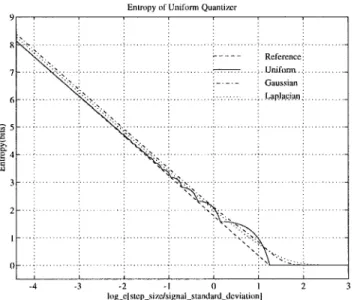
Fig. 2. Entropy of uniform quantizer for sources of different probability density functions (PDF’s).
Fig. 3. Mean square error of uniform quantizer for sources of different PDF’s.
A uniform midtread quantizer (in which zero is a recon-struction level) is often used in a practical coding system. Typically, the reconstruction levels are the centers of the
decision regions, i.e., , where
is the quantization step size. The behavior of such a quantizer has been analyzed for inputs with known probability distributions. Except for the uniform distribution, closed-form closed-formulas of entropy, , and distortion, , for arbitrary probability distributions are generally unavailable. The formulation of and for uniform, Gaussian, and Laplacian distributions are described in the Appendix. The numerical values of these functions are plotted in Figs. 2 and 3. The “Reference” curves in Figs. 2 and 3 are computed using (9) and (10) with (see below).
It is known that, at high bit rates (small distortion), the bits ( ) versus distortion ( ) relation of an entropy-coded uniform quantizer for a zero-mean i.i.d. source can be
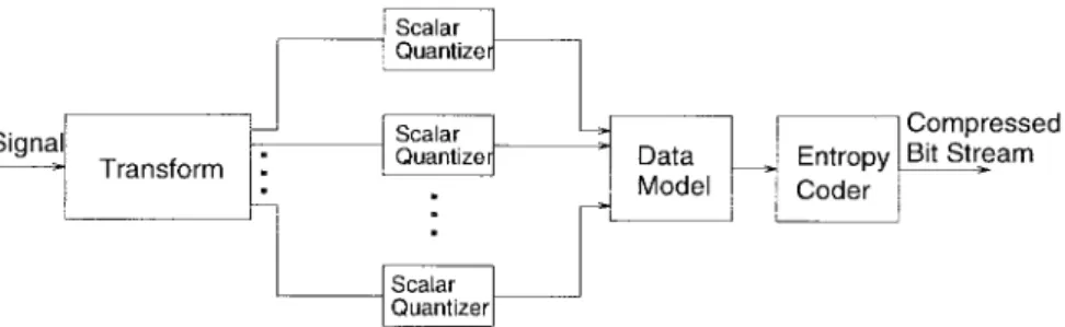
Fig. 4. Practical image transform coder.
approximated by the following formulas [4], [12]:
(9) and
(10) Thus
(11) where is 12 and is 1.386 ( ) for uniform, Gaussian, and Laplacian distributions, is source dependent and is about one for uniform distribution, 1.4 for Gaussian, and 1.2 for Laplacian, and is the signal variance. As shown by Figs. 2 and 3, the above approximations are fairly accurate when the quantization step size is smaller than the signal standard deviation. Combining (9) and (10) we obtain
(12) This gives us a more direct relation between and .
In image coding, bits are typically spent on a small percent-age of dominant transform coefficients of which the allocated bit rates are often higher than a couple of bits per coefficient. Although there is no simple and accurate formula for the low variance coefficients, these coefficients do not affect the overall model very much since their contribution in bits is relatively small. Therefore, the above formulas, although are accurate for medium to high bit rates, they are still practically useful for all the bit rates of interest.
In a real system, the ideal entropy coder is typically replaced by a variable-length coder (VLC), a simplified version of Huffman code [13]. Assuming this VLC is nearly as efficient as the ideal entropy coder, the bits produced by this VLC, , may be approximated by , where is the ideal entropy bits of the quantizer outputs, and is a scaling factor (for adjustment) greater than one. Under this assumption, (12) may still be used for a practical scalar quantizer with a modified value of (to be discussed in Section V).
III. PRACTICAL TRANSFORM CODER
A practical image transform coder, such as the DCT coders used in [1]–[3], can be represented by the general block diagram in Fig. 4. It follows roughly the aforementioned
principles, namely, a transform (DCT) used to decompose the original pictures into nearly independent components, a uniform scalar quantizer used to reduce the output levels, and a VLC used to further compress the output bit stream. As compared to that described in Sections II-A and II-B, the in-dividual entropy coders are replaced by a data model followed by an entropy coder. The objective of transformation and data model together is to produce (nearly) statistically independent data sequences so that they can be coded separately with high efficiency.
The data model used in [1]–[3] simply rearranges the transform coefficients in a zigzag scan order. That is, the 2-D array of a block of DCT coefficients are assembled to form a zigzag scanned 1-D linear array or vector
, in which the lower frequency’s DCT co-efficients are usually associated with smaller indices. When the coefficients are ordered in this fashion, the variances of coefficients are approximately monotonically decreasing [2].
If the transformed source vector is
stationary and every frequency component is independent, then the average entropy per block, , equals the sum of the entropies of all the components.
According to [12] and [14], the conditions discussed in the above, to a great extent, satisfied; that is, the frequency components (transform coefficients) are nearly i.i.d. sources, the distortion of quantized coefficients are relatively small, and the VLC performance is close to that of the ideal entropy coder. Then, the behavior of such a transform coder can be derived from (9) or (11) by combining all the components together. Assuming the probability distribution of the fre-quency components is either uniform, Gaussian, or Laplacian, and is the average bits of the th entropy-coded, quantized coefficient, the total average bits of such a source is
(13)
(14)
where , , and are the distortion, the variance, and the parameter associated with the th component. Since
(10)
where is the quantization step size of the th component, and is the parameter associated with that component.
Due to the frequency-dependent visual sensitivity of human perception [12], bits assigned to a frequency component should be adjusted according to their perceptual threshold. Thus, the quantization step size of each transform coefficient, , can be different in JPEG [2] and MPEG [3]. In addition, the quantization step sizes in MPEG are made of two components: , a quantization scaling factor for the entire picture block, and , a weighting matrix whose elements are used as multiplicative factors to produce the true step sizes in quantization. In other words, . On the other hand, the H.261 specification assumes that all the step sizes in a block are identical [1], that is, for all . The frequency-dependent step size design implies a frequency-weighted bit allocation scheme discussed in Section II-A in the sense that some frequency components get assigned fewer bits because their actual step sizes used in quantization are larger; that is [from (12)]
(16) Therefore, (14) and (15) become
(17) with
and
(18) They completely describe the bits and distortion behavior of an MPEG or JPEG transform coder under the ergodic Gaussian signal assumption. A special case that and for all has been reported in [7].
In reality, a frequency component may have an effective
variance less than the weighted distortion, . Also, as the theory predicts, the value of is close to 12 when is much higher than , but its value may be different if is close to or smaller than . We then need to go back to (3) and (4), and modify (17) and (18) to the following:
(19) (20) where regions of and are
and
is the size of set , and
Using optimization techniques, Netravali and Haskell derived similar but not identical results under the frequency-weighted distortion criterion [12].
IV. THRESHOLDTRANSFORM CODER
In digital image coding, theory and practice do not agree completely due to several nonideal factors. First, the assump-tions undertaken by theory (in the previous secassump-tions) such as ergodicity and stationary of image sources do not hold exactly on real data. Second and more importantly, the human visual system is highly nonlinear and cannot be approximated by a simple distortion measure such as the mean square error (MSE). For example, a very small percentage of a coded picture bearing visible artifacts does not affect the overall MSE very much; however, a human viewer can easily pick up the distorted areas, and thus the entire picture quality is rated low. Therefore, in image coding we have to deal with not only the statistical behavior of the entire picture (objective criterion) but also the fidelity of individual samples embedded in their texture neighborhood (subjective criterion).
Several intuitive schemes have been proposed to solve the above problem. Instead of selecting a fixed number of transform coefficients according to their average variances as suggested by the theory, we select the coded coefficients by their magnitudes, the so-called threshold transform
cod-ing. The direct implementation of threshold coding requires
transmitting the threshold mask—locations of the chosen co-efficients—which often needs a significant number of bits. A popular approach is rearranging the transform coefficients in a fixed scanning order, transmitting them sequentially until the last above-threshold coefficient is hit, and then appending an end-of-block code to conclude this data block. The exact analysis of such a coder is involved and may not be worth the efforts since the real image data do not match exactly our stationary model assumption. The following simplification seems to be sufficient for image coding purpose.
Our focus is on the bit-distortion model, i.e., the average bits and distortion associated with a typical block. Assuming that is the threshold value used in picking up the th transform coefficient; that is, the th coefficient is set to zero before quantizing if its magnitude is less than . A popular variant of this scheme is the dead zone quantizer—the decision region of the zero reconstruction level is larger than the decision region used for the other reconstruction levels. In both cases and the combined situation, the analysis of such quantizers is similar to that of a simple uniform quantizer; however, the decision levels and the reconstruction levels have to be modified in the analysis equations. Details of the above modifications are described in the Appendix.
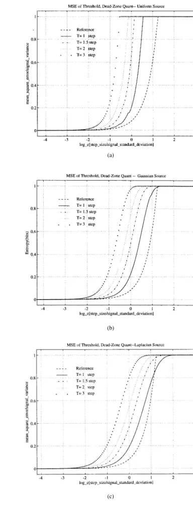
For various threshold ( ) values, the entropy versus dis-tortion curves of a uniform quantizer with a dead zone set
(a)
(b)
(c)
Fig. 5. Entropy of quantizers with dead-zone for (a) uniform, (b) Gaussian, and (c) Laplacian sources.
(a)
(b)
(c)
Fig. 6. MSE of quantizers with dead-zone for (a) uniform, (b) Gaussian, and (c) Laplacian sources.
Reference curves shown on those plots are the asymptotic
formulas described by (9) and (10).
In image coding, the quantization step sizes of significant frequency components are usually smaller than the signal standard deviation; therefore, (10) and (12) are reasonably good approximations if , , and are adjusted appropriately. The values of these parameters, in general, depend upon and . However, for a fixed and a certain range of step sizes, they can be approximated by constants. When the step size gets larger, (10) and (12) become less accurate. But in these cases the bits produced by those coefficients are very small and thus do not change very much the total bits. Extensions and modifications of these parameters are described in the next section.
Assuming that the bits on the average needed to encode an above-threshold transform coefficient are represented by [from (12)]
(21)
where , is the threshold value used in picking up the th transform coefficient, and and are source-dependent parameters. The average bits number of a pixel becomes
(22)
where are the bits for the end-of-block signal.
If the weighting matrix in (17) is adopted, the average bits and the average distortion can be made more explicit
(23) and
(24)
Since the threshold transform coding with weighting matrix is invented to match the subjective distortion criterion, the mean square error distortion calculation, (24), is not as useful as the bits calculation, (23), which can be used to adjust the quantization step for regulating encoder buffer and controlling picture quality.
If is chosen to be with roughly
the same constant value for all the coefficients, then , , and can be expressed as functions of and only. Also, in most image coding cases, the ac components have approximately Laplacian distribution and the dc component, uniform or Gaussian distribution [12]. Hence, the values are similar for all the frequency components as indicated by Fig. 5, in which ’s are proportional to the slopes of
these curves and have about the same value for all the three distributions. Therefore, replacing in (23) by , we obtain (25) where (26) Or (27)
with . Note that we denote by
in the above equations for simplicity.
The direct use of (25) seems to be fairly complicated—it needs to estimate a number of parameters, ’s, ’s, and , computed from image data. If, however, we could assume that the picture to be coded is not much different from the picture that has already been coded in the sense that the , and remain about the same in the neighborhood of that we are dealing with, then the parameter in (27) can be estimated from the and of the coded pictures. Typically, the value is less picture-dependent, only the value has to be estimated from image data. Consequently, the entire model identification procedure can be relatively simple.
V. MODEL PARAMETERS
For a practical application, the parameters of the above model have to be adjusted to cope with the specific video coder used and the real picture characteristics. The meaning of the parameters in our model (23) and (24) suggests the following modifications. First, since is a factor mainly determined by probability distribution, we assume is a constant ( 1.2 for Laplacian source, say) for the rest of analysis. Second, the value of is no longer constant for small ; however, those values can be precalculated and stored in a table for real-time applications. Third, the constant
is replaced by a parametric function
to compensate for the mismatch between the ideal model and a practical video coder. Although these parameters ( , , and ) may be somewhat related, for simplicity we study them separately. We will elaborate on the second and the third items below.
A. Model Parameter
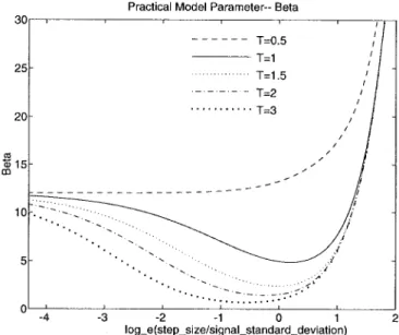
We wish to find the model parameter for different and under the assumption that is a constant ( 1.2). If the quantization error is i.i.d. and is uniformly distributed, the theoretical value of is 12. This is approximately true when the quantization step is much smaller than the signal variance (the left portion of Fig. 7). However, the above assumption is not valid for large quantization step sizes. Since the high frequency transform coefficients are roughly Laplacian distributed, we are interested in the Laplacian cases. Combining (21) and (A9) in the Appendix, we obtain the
value for the Laplacian probability distribution (28)
The values calculated based on this formula are plotted in Fig. 7. From Fig. 7, we find that increases abruptly after exceeds a threshold value ( 1.3). This is because when the quantization step size is very large (comparing to the signal variance), quantization errors can no longer be treated as uniformly distributed. Therefore, the distortion goes up at a slower pace than the asymptotic formula predicts. Eventually, the distortion saturates when it approaches the signal variance (Fig. 6). However, in order to use the same distortion function, (10), for the cases that their distortion is approaching signal variance, the corresponding values are made growing exponentially (Fig. 7). In real-time applications, it is not likely to compute directly based upon the above equations. For a specific system, MPEG say, we choose a fixed ( in this instance) and build a look-up table for real-time use. We did the same thing in the following simulations. One may note from Fig. 5(c) that entropy 0 when . Hence the look-up table needs only to store the values for smaller than 1.5. For 1.5, the corresponding distortion value is , and in this case, based on the original definition of in (10), becomes . On the other extreme for
, a constant of 12 is assigned to .
B. Nonideal Factors in a Practical Coder and Parameter
Mismatches between the theoretical entropy model and the real VLC coded bits are discussed in this section. Several scal-ing factors are observed and estimated from experimental data to compensate for the mismatches. In Section II, is initially treated as constant ( 1.386), but later analysis suggests that varies depending upon the value of quantization step size. First, the probability density functions (PDF’s) of the ac coefficients are not ideal Laplacian distribution of equal vari-ance. This PDF mismatch, shown in Fig. 8, results in a smaller entropy for real transform coefficients than the predicted value based on Laplacian assumption. As the quantization step increases, the probability of the quantized values around zero grows much larger than that of the other intervals, and the PDF mismatch problem becomes even more serious. We thus introduce a multiplicative factor to compensate for the difference. Second, the transform coefficients within a block
Fig. 7. Model parameter for various dead-zone values (T ) and quantiza-tion step sizes (delta).
are somewhat correlated; hence, another multiplicative factor, , is introduced to correct the original i.i.d. assumption. Third, the VLC table in image coding standards is built based on the probability of zero coefficient runs and coefficient
levels, (run, level), rather than on .
Therefore, the average encoded bits per block are higher than the theoretical block entropy. We denote this inefficiency of VLC table by the third multiplicative parameter . Combining these factors together as a whole, we obtain
bits
bits (29)
where bits represents the real coded bits. All the above multiplicative scaling factors are functions of quantization scale ( ). Hence, the overall factor is, in general, a function of . Practically, we only need to estimate the overall factor from the real data. Therefore, (27) is still valid when is replaced by bits , as long as the new includes the nonideal factor .
In summary, the original [ in (25) and (27)] is now
replaced by , where is a function of ,
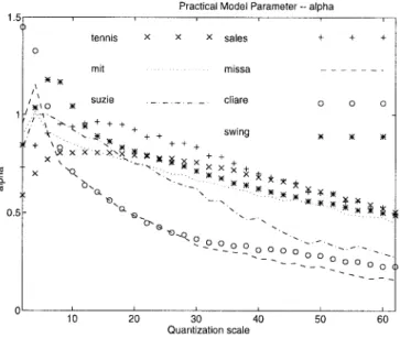
and it includes the nonideal factors in entropy coding. Once we decide the value (Section V-A), (27) can be used to compute from data. An H.261-type coding structure is used as an example. Since the dc coefficients are coded with fixed length codewords and their coding is independent of the ac coefficients coding, we concentrated on the statistical analysis of the ac coefficients. Fig. 9 shows the values computed from the intracoded frames of several video sequences at different values. In this experiment, the values are taken from Fig. 7, is set to “1” for all the frequency components, and is neglected.
(a)
(b)
Fig. 8. Probability density functions (solid line) of the first ac component of transform coefficients for (a) Salesman and (b) Claire. The dash lines are Laplacian density functions of the same variance, and the dotted lines are Gaussian density functions of the same variance.
It can be seen that the values are getting larger and approaching one when the quantization scales are getting small. This is because the quantized coefficients are less correlated at small quantization scales. Hence, the encoded bits are well estimated by our original entropy model. For larger quantization step sizes, the original model predicts fewer bits than the true bits. To compensate for this fact, is significantly smaller than one for large .
In order to use our model in predicting coded bits, we look for a simple arithmetic expression of . A first-order linear curve fitting is obtained from experimental data as follows:
(30) where and are two picture dependent constants. Since is an indication of image complexity, we derive the following empirical formulas for typical values of and
Fig. 9. Model parameter s(qs) for various pictures.
and .
Thus far, we have obtained the parametric formulas of and . These expressions can be used to estimate the bits needed to encode a picture with a prechosen quantization scale.
C. Bits Prediction
If the coded bits can be predicted prior to the quantization and VLC operations, then the coding process can be well controlled. Based on (25), (27), and the parameters and described in the preceding subsection, bits needed to encode a picture for a given distortion (quantization step) can be estimated if the variances of transform coefficients are available. The picture characteristics from coding point of view are completely specified by the function in (27). This function, , can thus be considered as the measure of picture coding complexity and therefore is named “coding
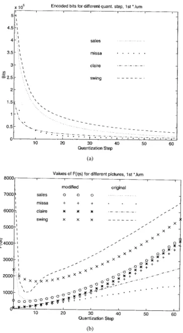
complexity function.” If we keep in (27) as a constant and allow to vary to accommodate for the varying , the computation in quantizer control procedure can then be simplified somewhat. In this case, the resultant is called “modified ” and is denoted by . For easy distinction, we call the “original ” denoted by if it is computed using (27) directly based on the variances of block transform coefficients. Some examples of and are shown in Fig. 10. An interesting observation is that both and can be approximated rather well by a linear equation (for each picture separately) when ’s are relatively small (between 10 and 30), which are the most frequently used values in practice. In other words
(31) where and are two picture-dependent constants. We can see from Fig. 10(a) and (b) that the coded bits of different pictures are reflected on their corresponding coding complexity functions. If the picture contents do not change significantly
(a)
(b)
Fig. 10. The coding complexity function for various pictures (the first frame in those picture sequences). (a) Coded bits per pixel for various quantization step sizes and (b) the modifiedF (qs)(Fm(qs)) and the original
F (qs)(Fo(qs)) values.
between two nearby frames, the computed from the previous frame can still be used to estimate the bits of the current frame at similar step sizes.
We should keep in mind that the above bits model is derived based on several assumptions of the statistical behavior of data. For real pictures and picture sequences, the stationarity and ergodicity assumptions are not completely satisfied. In addition, this simple model uses essentially only to estimate the bits needed to encode an entire picture. Although is made a function of , it is not possible to cover all the nonstationarity and data-dependency fully by only a couple of parameters. Therefore, a small amount of estimation errors cannot be avoided.
VI. CONCLUSIONS
In this paper, we derive a source model that describes the relationship between bits, distortion, and quantization
step sizes for block-transform coders. This source model is initially derived based on rate-distortion theory. The realistic constraints such as quantizer dead-zone and threshold coeffi-cient selection are included in our formulation. The picture complexity from a coding point of view can be measured and computed from the entropy variance which is the product of all the component’s variances of image signals. When the model is used in real video coding, image characteristics and nonideal factors of a practical video coder are accommodated by parameterizing the model constants. If the parameter values are properly chosen, the coding behavior can be well estimated by the proposed model. In brief, there are two aspects of our contribution. One, we extend the existing results of rate-distortion theory to the practical video coders, and two, the nonideal factors in real signals and systems are identified and their mathematical expressions are derived from experimental data. One application of this source model, as shown in the second part of this paper, is the buffer/quantizer control in video coders with the advantage that the picture quality is kept nearly constant over the entire picture sequence.
APPENDIX
ENTROPY AND DISTORTION OF UNIFORMLY QUANTIZED UNIFORM ANDLAPLACIAN SOURCES A. Uniform Quantizer
The behavior of a uniform quantizer can be analyzed by the following equations for inputs with known probability distributions. Assuming that the probability density function of a zero-mean i.i.d. source is , the entropy bits produced by this uniform quantizer can be calculated by
(A1)
where
(A2) and the mean square quantization error is
(A3)
where decides the total number of quantization levels ( ), chosen sufficiently large to eliminate almost all the overloaded quantization errors.
B. Uniform Distribution
Assuming that a zero-mean uniform distribution i.i.d. source with variance is quantized by a uniform quantizer described above. Then, the entropy of the outputs is [5]
and the mean square quantization error is
(A5)
C. Gaussian Distribution
The probability density function of a zero-mean Gaussian source with variance is
Unfortunately, there are no closed form formulas of (A1) and (A3) for Gaussian distribution. However, in this case, it is not difficult to compute their numerical values using (A1) and (A3). The results are shown in Figs. 5(b) and 6(b). When is reasonably small, the PDF is approximately constant in a -width interval. We then obtain the asymptotical behavior of such a quantizer at high bit rates as indicated by (9) and (10).
D. Laplacian Distribution
The probability density function of a zero-mean Laplacian source with variance is
Thus
(A6) The general formulas of entropy and distortion of uniformly-quantized Laplacian source with dead-zone are given below.
E. Dead Zone
Assume that the first reconstruction level of a quantizer with dead-zone is , then the reconstruction levels are
If the corresponding input decision regions are selected as
then (A2) and (A3) are modified to
(A7) and
(A8)
For Laplacian distribution, let , and
.
The entropy (in bits) and distortion can be derived
(A9) and
(A10)
If we take the centroid of the decision region as the reconstruction level, we obtain
(A11)
A uniform quantizer without dead zone may be considered as a special case of the above with . In this case, the corresponding entropy and distortion are
(A12) and (A13) where (A14) F. Threshold
If a dead-zone quantizer also has a threshold and , then (A7) and (A8) are modified to
otherwise
and
(A16)
where
and represents the smallest integer that is greater than or equal to . When , the threshold operation is not effective. It then simply becomes a regular uniform quantizer.
REFERENCES
[1] CCITT, Working Party XV/1, “Draft of recommendation H.261: video codec for audiovisual services atP 2 64k bits/s,” July 1990. [2] W. B. Pennebaker and J. L. Mitchell, JPEG—Still Image Data
Com-pression Standard. New York, NY: Van Nostrand Reinhold, 1993. [3] MPEG (Motion Picture Experts Group, ISO–IEC JTC1/SC29/WG11),
“Coding of Moving Pictures and Associated Audio,” CD 11172-2 Nov. 1991.
[4] H. Gish and J. N. Pierce, “Asymptotically efficient quantizing,” IEEE Trans. Inform. Theory, vol. IT-14, pp. 676–683, Sept. 1968.
[5] N. S. Jayant and P. Noll, Digital Coding of Waveforms. Englewood Cliffs, NJ: Prentice Hall, 1984.
[6] T. Berger, Rate Distortion Theory. Englewood Cliffs, NJ: Prentice Hall, 1971.
[7] H.-M. Hang et al., “Digital HDTV compression using parallel motion-compensated transform coders,” IEEE Trans. Circuits Syst. Video Tech-nol., vol. 1, pp. 210–221, June 1991.
[8] A. Puri and R. Aravind, “Motion-compensated video coding with adaptive perceptual quantization,” IEEE Trans. Circuits Syst. Video Technol., vol. 1, pp. 351–361, Dec. 1991.
[9] W.-Y. Sun, H.-M. Hang, and C. B. Fong, “Scene adaptive parameters selection for MPEG syntax based HDTV coding,” in Signal Processing of HDTV, L. Stenger et al., Eds. Elsevier Science, 1994, vol. V. [10] A. J. Viterbi and J. K. Omura, Principles of Digital Communications
and Coding. New York, NY: McGraw-Hill, 1979.
[11] A. V. Oppenheim and R. W. Schafer, Discrete-Time Signal Processing. Englewood Cliffs, NJ: Prentice Hall, 1989.
[12] A. N. Netravali and B. G. Haskell, Digital Pictures: Representation and Compression. New York, NY: Plenum, 1988.
[13] R. E. Blahut, Principles and Practice of Information Theory. Reading, MA: Addison-Wesley, 1991.
[14] K. R. Rao and P. Yip, Discrete Cosine Transform: Algorithms, Advan-tages, Applications. San Diego, CA: Academic, 1990.
Hsueh-Ming Hang (S’79–M’84–SM’91) received
the B.S. and M.S. degrees from National Chiao Tung University, Hsinchu, Taiwan, in 1978 and 1980, respectively, and the Ph.D. in electrical engi-neering from Rensselaer Polytechnic Institute, Troy, NY, in 1984.
From 1984 to 1991, he was with AT&T Bell Laboratories, Holmdel, NJ, where he was engaged in digital image compression algorithm and architec-ture researches. He joined the Electronics Engineer-ing Department of National Chiao Tung University, Hsinchu, Taiwan, in December 1991. His current research interests include digital video compression, image/signal processing algorithm and architecture, and digital communication theory.
Dr. Hang was a conference co-chair of Symposium on Visual Commu-nications and Image Processing (VCIP), 1993, and the Program Chair of the same conference in 1995. He guest co-edited two Optical Engineering special issues on visual communications and image processing in July 1991 and July 1993. He was an Associate Editor of IEEE TRANSACTIONS ONIMAGE PROCESSINGfrom 1992 to 1994 and a Co-Editor of the book Handbook of Visual Communications (Academic Press, 1995). He is currently an Editor of Journal of Visual Communication and Image Representation, Academic Press. He is a member of Sigma Xi.
Jiann-Jone Chen was born in Chong,
Tai-wan, R.O.C., in 1966. He received the B.S. and M.S. degrees in electrical engineering from National Cheng Kung University, Tainan, in 1989 and 1991, respectively. He is currently working toward the Ph.D. degree in electronics engineering at National Chiao Tung University, Hsinchu, Taiwan.
His research interests include medical image pro-cessing and digital video coding.