以部分法修正地理加權迴歸 - 政大學術集成

全文

(1)國立政治大學統計學系碩士論文. 學. ‧ 國. 立. 政治大. A Conditional Modification to. Geographically Weighted Regression. ‧. n. er. io. sit. y. Nat. al. Ch. engchi. i n U. 指導老師 : 余清祥博士研究生 : 梁穎誼. 中華民國一百年六月. v.

(2) 謝誌. 當初在 Malaysia 什麼都不懂，來到了這塊地方。或許來之前就已經找好人生方向了，來的這裡就一直讀書，貪婪的吸取統計的知識。結果一直讀書啊，一直讀書。不知不覺讀了八年。歲月不留人，人老的特別快，以前還能蹦蹦跳跳，現在動久了就會 sakit 到鬼這樣。驚覺回頭，才發現要獲得知識並不是沒代價的，除了口袋有形的 RM(或 NTD)，還必須付出無形的健康跟時間。錢能找的回來，其它是很難的。給所有看到這篇的人，研究之餘請注意健康。台灣其實是一個學術風氣不錯的地方。我必須感謝台灣這塊土地。很幸運的，. 治政我在台灣遇到很多貴人。其中，我想最應該感謝的是余清祥老師，老師不但在學大立術上給予了我良好的指導，而且也好幾次雪中送炭，讓我能夠無後顧之憂完成了 ‧ 國. 學. 這份研究。我想這篇論文有一半應屬於老師的。另外，我也必須感謝江老師，雖. sit. y. Nat. 我。. ‧. 然在碩士階段的交集不多，不過每次我找老師幫忙，即使老師在百忙之中還幫助. io. er. 此外，還有其他的人，包括一起學習的貝姐、BRK、燴飯、OOO。一起 drink drink 的損友。還有 mee gia, gai gai, old papa 等。Terima Kasih。. n. al. Ch. engchi. i n U. v.

(3) 中文摘要在二十世紀九十年代，學者提出地理加權迴歸（ Geographically Weighted Regression;簡稱GWR)。GWR是一個企圖解決空間非穩定性的方法。此方法最大的特性，是模型中的迴歸係數可以依空間的不同而改變，這也意味著不同的地理位置可以有不同的迴歸係數。在係數的估計上，每個觀察值都擁有一個固定環寬，而估計值可以由環寬範圍內的觀察值取得。然而，若變數之間的特性不同，固定環寬的設定可能會產生不可靠的估計值。為了解決這個問題，本文章提出CGWR(Conditional-based GWR)的方法嘗試修正估計值，允許各迴歸變數有不同的環寬。在估計的程序中，CGWR. 政治大也同時透過電腦模擬比較GWR, CGWR與local linear法(Wang and Mei, 2008) 立的表現。研究發現，當迴歸係數之間存有正相關時，CGWR比其他兩個方法運用疊代法與交叉驗證法得出最終的估計值。本文驗證了CGWR的收斂性，. ‧ 國. 學. 來的優異。最後，本文使用CGWR分析台灣高齡老人失能資料，驗證CGWR 的效果。. ‧ y. Nat. 模擬、MAUP問題. n. al. Ch. engchi. er. io. sit. 關鍵字 : 地理加權迴歸、廣義加法模型、交叉驗證法、Jacobi疊代法、電腦. i n U. v. I.

(4) Abstract. Geographically weighted regression (GWR), first proposed in the 1990s, is a modelling technique used to deal with spatial non-stationarity. The main characteristic of GWR is that it allows regression coefficients to va ry across space, and so the values of the parameters can vary depending on locations. The parameters for each location can be estimated by observations within a fixed range (or bandwidth). However, if the parameters differ considerably, the fixed bandwidth may produce unreliable or even unstable estimates. To deal with the estimation of greatly varying parameter values, we propose. 治政 each independent variable. The bandwidths 大 for the independent variables are 立 algorithm using cross- validation. In addition to showing derived via an iteration Conditional-based GWR (CGWR), where a different bandwidth is selected for. ‧ 國. 學. the convergence of the algorithm, we also use computer simulation to compare the proposed method with the basic GWR and a local linear method (Wang a nd Mei,. ‧. 2008). We found that the CGWR outperforms the other two methods if the. n. er. io. al. sit. Nat. from Taiwan to demonstrate the proposed method.. y. parameters are positively correlated. In addition, we use elderly disability data. i n U. v. Keywords: Geographically weighted regression, Generalized additive model,. Ch. engchi. Cross validation, Jacobi iteration, Computer simulation, Modifiable areal unit problem. II.

(5) Index 1. Introduction ----------------------------------------------------------------------------- 1 2. GWR and its extension ---------------------------------------------------------------- 2 2.1 GWR --------------------------------------------------------------------------------- 2 2.2 Local linear method -------------------------------------------------------------- 6 2.3 Drawbacks ------------------------------------------------------------------------ 7 3. Methodology -------------------------------------------------------------------------- 9 3.1 Generalized Addictive Model --------------------------------------------------- 9 3.2 Jacobi Iteration --------------------------------------------------------------------- 9 3.3 Proposed CGWR ----------------------------------------------------------------- 10 4. Simulation Study -----------------------------------------------------------------------15. 治政大 4.2 Single type surfaces --------------------------------------------------------------19 立 4.3 Mixed type surfaces ---------------------------------------------------------------25 4.1 Simulation Setting ---------------------------------------------------------------- 16. ‧ 國. 學. 4.4 Random effect model ------------------------------------------------------------- 27 5 Empirical Study ------------------------------------------------------------------------- 30. ‧. 6. Discussion and Concluding Remarks ---------------------------------------------34. n. er. io. sit. y. Nat. al. Ch. engchi. i n U. v. III.

(6) Table Index Table 1-1 The average discount rates on a linear surface (single-type) ---------20 Table 1-2 The average discount rates on a quadratic surface (single-type) ----- 20 Table 1-3 The average discount rates on a ridge surface (single-type) --------- 21 Table 1-4 The average discount rates on a hillside surface (single-type) ------- 21 Table 2 The average bandwidths for linear and hillside surfaces (single-type)--22 Table 3-1 The average variances and biases of B0 and B1 on a linear surface -- 23 Table 3-2. The average variances and biases of B0 and B1 on a ridge surface -- 24 Table 4-1 The average discount rates of a linear-quadratic surface --------------- 26 Table 4-2 The average discount rates of a ridge-quadratic surface --------------- 26 Table 5-1 The average discount rates on a linear surface (random effect). ------27. 治政大surface (random effect). -------28 Table 5-3 The average discount rates on a ridge 立 Table 5-4 The average discount rates on a hillside surface (random effect). ----29 Table5-2 The average discount rates on a quadratic surface (random effect) ---28. ‧ 國. 學. Table 6 The correlations of the independent variables from the disability data. 31. ‧. Figure Index. y. Nat. Figure 1 Four coefficient surfaces. ------------------------------------------------------ 18. sit. Figure 2 The B1 mean surface of each estimation method from 100 simulations.22. al. er. io. Figure 3 The surface of Intercept and variable POP from different fitting method.. n. iv n C Figure 4 The residual plots h & Residual histogram e n g c h i U of the GWR,Local. ------------------------------------------------------------------------------------- 32. linear method and CGWR. ---------------------------------------------------- 33. Figure 5 Average discount rate of each method by fixing variable x2------------- 36. IV.

(7) Chapter 1. Introduction In recent years, spatial regression has become an important tool for analyzing spatial data. In applying the analysis, first order stationarity is a common assumption and the expected values at different locations are assumed to be fixed. Thus, similar to the development of time series analysis, the focus of spatial regression is on the covariance structure. Some well-known spatial covariance models such as Simultaneous autoregressive (SAR) and moving. 政治大. average (MA) can be treated as spatial versions of the AR and MA models used in. 立. the time series analysis. However, first order stationarity is a questionable. ‧ 國. 學. assumption in practice. For example, the term Modifiable areal unit problem. ‧. (MAUP), used in the geography, particularly on the scaling effect can be treated. sit. y. Nat. as a spatial version of Simpson Paradox, is often encountered when dealing with. io. al. er. spatial data. Other than the problem that the parameters’ values are not identical in. n. all locations, including the data with different attributes for estimation may also produce biased results.. Ch. engchi. i n U. v. In other words, estimating the parameters using all of the data and the ordinary least squares (OLS) method would distort the local distinctness. One possible solution is only considering the data from areas with similar attributes. However, it is difficult to define the locations of homogeneity. Moreover, the mean of a non-stationary process is usually continuous across the space and does not follow a step- function (Fotheringham et al., 2002), making it difficult to find the exact boundary of the appropriate data points. The other possibility is the varying coefficient model (Cleveland et al., 1991). The model allows the coefficient terms being a functiona l form of a scalar, 1.

(8) which is related to locally linear models (Fan and Zhang, 2008). Note that, the varying coefficient model has been plugged into different kinds of application such as survival analysis, time series model, etc, and is a popular tool to explore the dynamic feature. Based on the concept of varying coefficient model, geographically weighted regression (GWR) was proposed to solve the problem of MAUP (Brunsdon et al., 1996). The GWR allows the regression coefficients to vary across the space or map. It is used to obtain estimates from a moving data window and is analogous to kernel regression for obtaining a smoothing estimate. The OLS can be treated as a. 政治大. special case of GWR, i.e., a window with infinite length, but the local distinctness. 立. is likely to be lost by averaging all of the observations. The optimal length (or. ‧ 國. 學. bandwidth) of the moving windows in GWR is usually determined by cross-. sit. y. Nat. variables.. ‧. validation (CV) or Akaike’s information criterion (AIC), and is fixed for all. io. al. er. Nevertheless, there is still room for improvement, mainly related to the selection and testing of the bandwidth. For example, using CV and AIC to select. n. iv n C the optimal bandwidth is a h data-driven method, e n g c h i U and like in kernel regression, the estimates are sensitive to outliers (Farber and Páez, 2007). In addition, the data variations are not necessarily the same and the bandwidth should not be fixed as well. On the other hand, the hypothesis testing of the parameters depends on the bandwidth. For example, Leung et al. (2000) proposed some goodness-of-fit tests and found that the degree of freedom of GWR residuals is a function of the bandwidth. Since selecting the bandwidth can be somewhat subjective, it is possible to come up with totally different results by using different tests. Several GWR modifications were proposed since its introduction, most of which are related to determining the bandwidth. Brunsdon et al. (1999) introduced 2.

(9) a mixed GWR model that allows the inclusion of both stationary and nonstationary coefficients. They also proposed vector bandwidths, allowing coefficients with different bandwidths via a backfitting algorithm and bandwidths that were functions of data density. Shi et al. (2006) proposed a weighting function that allows the GWR spatial weight to be influenced by the attribute, rather than the distance. Furthermore, Farber and Páez (2007) found that it is possible to reduce the bias by modifying the CV procedure. Recently, Wang et al. (2008) introduced a local linear estimation, or a polynomial fitting technique, to reduce the bias.. 政治大. However, in spite of these GWR modifications, the issue that the variations. 立. of each coefficient can be very different has not yet been discussed in details.. ‧ 國. 學. Intuitively, it is reasonable to provide separate bandwidths if the coefficients. ‧. behave differently. Under the classic GWR setting, the bandwidth is the same for. y. sit. io. al. er. smoothed.. Nat. all of the coefficients and the estimates are likely to be over-smoothed or under-. Meanwhile, enormous data analysis based on GWR showed that the. n. iv n C correlations often exist between coefficients. Despite most of them didn't h e nGWR gchi U mention the exact index, the correlations are apparent through the outcome mapping. Bivand and Brunstad (2005) even calculated the correlation index, which is nearly high correlated. Note that, the correlation can be additional information to improve the estimation, as the Control variant technique on Variance reduction. Therefore, the information should be sufficiently use rather than ignore it. Although the problem we are dealing with is not entire identical in variance reduction, the idea can be borrowed to modify the estimator. To complete the puzzle, in this paper, we propose a method to provide separate bandwidths for different coefficients via an iteration algorithm. We also 3.

(10) evaluate the validity of the proposed method by comparing it with the basic GWR and local linear method by Wang et al. (2008). The next section will first introduce the GWR and its extension. Next, Section 3 will introduce proposed method, namely Conditional-based GWR (CGWR), and its theoretical results. Section 4 discusses simulation studies of comparing the performance of the proposed method with that of the basic GWR and local linear method. In addition to simulations, we also apply the proposed method to a real data set, as shown in Section 5. Section 6 provides a discussion of the proposed method that includes its limitations and scope for possible future developments.. 立. 政治大. ‧. ‧ 國. 學. n. er. io. sit. y. Nat. al. Ch. engchi. i n U. v. 4.

(11) Chapter 2. GWR and its extension 2.1 GWR We shall first provide a brief introduction of the GWR, followed by an introduction of the proposed method. The GWR uses a dependent variable y modelled as a linear function of a set of p independent variables, x1, x2 ,  , x p , and can be expressed as p. Yi  i 0   ik xik   i ,. 政治大 are the parameter and observed value of variable k 立. (1). k 1. where  ik and xik. (k  1, , p ). ‧ 國. 學. for observation i, respectively, and  i is the error term for observation i, which is generally assumed to be from a normal distribution with zero mean and constant. ‧. variance  2 (i.e.,  i ~ N (0,  2 ) ). The subscript i represents the spatial location. y. Nat. er. io. sit. of observation i (i  1,, n) . In other words, in the GWR model, each location can be thought of as having its own regression model for the dependent variable. n. al. Ch. i n U. v. and independent variables. Thus, the essence of GWR is to obtain local regression. engchi. with nearby data for each location, and choosing an appropriate range for the data becomes a key factor. We will use the term “bandwidth” to represent this data range for the rest of this paper. The parameter set β i of observation i can be estimated by -1 T βî = (XT WX) X WiY , i. (2). where βî = ( βî0 , βî1 ,..., βîp )T , X = (1, x1 ,..., x p )T ,Y = (Y1 ,..., Yn )T , and Wi is a diagonal weight matrix. The weight matrix contains the weights of the neighbourhoods for the i th observation, and can be expressed as: 5.

(12)  0   wi1      Wi    wi j         0  win  . (3). where wij ( j  1,..., n ) are obtained by kernel functions. The kernel functions chosen are usually distance-weighted and Gaussian type, 1 wij  exp[- (dij / h) 2 ] 2. (4). However, if data locations are sparse at somewhere on the space, distance-. 政治大. weighted kernel might not appropriate due to lack of information. Brunsdon et al.. 立. (2002) introduced rank-based and k nearest neighbourhood method as the. ‧ 國. 學. solutions. In addition, as we mentioned before, bandwidth selection is generally calibrated via minimizing Cross-validation score or AIC.. ‧ y. Nat. io. sit. 2.2 Local linear method. n. al. er. Wang et al. (2008) proposed local linear-fitting-based GWR, which is. Ch. i n U. v. Taylor expansion version of GWR. The main essence of it is to reduce bias by. engchi. using second continuous partial derivatives with respect to geographical location coordinates. For any given location, the regression parameter can be locally approximated as.  j  ij  ij(u )(u  u0 )  ij v( (v)  v0 ) j  1, 2,..., p,. (5). where  j is any of regression parameter and  ij is the parameter of the given location. ij(u ) and ij( v ) are the partial derivatives of  j at location i, that is, two-dimensional coordinates on the location, with respect to each axis.. 6.

(13) To estimate the parameters, the matrix of independent variables can be simply rewritten as.  x1 1  x *  2 1 Xi =     xn1. x 1( 1 u1 i u). x (1 1 v. x 2( 1 u 2 i u) . x (2 1v . xn1( un u)i. x1n( vn. 1i 2i. )v )v . p. x1. p. p. x2. p. . )v i. x( 1 u 1i ) u x(  2 u 2i ) u  x( n p u. xn p. n. )u. (x1 v1i )  x( 2 v2i ) p    (x n pv )n p. i. v v (6) v. i. where u and v are the coordinates of the locations. By adding intercept into the * matrix,(i.e. X** i = (1, u - u i , v - v i , X i ) ), the parameters can be estimated by. ** T ** -1 ** T βî = ( X W ) X YW i i X i i i. (7). 政治大. which is similar to the original GWR estimator.. 立. ‧ 國. 學. 2.3 Drawbacks. Using a single bandwidth in the GWR is likely to create unsatisfactory. ‧. estimates if the corresponding surfaces of independent variables have different. y. Nat. io. sit. attributes (such as different shapes or variations). Allowing different bandwidths. n. al. er. seems to be a natural modification to the GWR. Unfortunately, the weighted. Ch. i n U. v. least squares and equation (2) cannot handle the situation of varying bandwidths. engchi. for different variables. Brunsdon et al. (1999) proposed an approach similar to a stepwise regression and backfitting algorithm for selecting different bandwidths. However, they did not provide suggestions for choosing bandwidths. Of course, choosing the optimal bandwidths is similar to the problem of minimization, and thus the methods such as grid search can be used. However, these methods usually require intensive computation and might not be feasible. Local linear method solves the aforementioned problems when all the coefficient surfaces are linear, since the remainder of the Taylor expansion would be zero in this case. In other words, all bandwidths are infinite and same due to 7.

(14) unbiasness. But, the method suffers from the bandwidth problem again when it is not the case. On the other hand, there is another problem that we should concern on local linear estimation. In such complex surface, the slope could different on different location, and we might expect this method would mislead the surface at somewhere slopes change rapidly, which mostly happen on non-linear surface. Finally, we would like to point that adding additional dependent variable could increase the variance too. In this study, we introduce an approach to determine different bandwidths. 政治大. using iteration. This approach is inspired by the vector bandwidth of Brunsdon et. 立. al. (1999) and by the kernel smoothing used in the varying-coefficient model of. ‧ 國. 學. Wu and Chiang (2000). We combine these ideas and propose a method (and an. ‧. algorithm to establish the estimation) for selecting each variable’s bandwidth. The. sit. y. Nat. proposed method uses some existing techniques such as the generalized additive. io. n. al. er. model (GAM) and the Jacobi iteration method, which will be mentioned first.. Ch. engchi. i n U. v. 8.

(15) Chapter 3. Methodology 3.1 Generalized Additive Model Hastie and Tishibirani (1990) proposed the GAM, replacing the linear function x k by a polynomial function of x k , or mk ( xk ) , in equation (1). This model can be written as: Yi  m0  m1 ( x1 )  m2 ( x2 )   m p 1 ( x p 1 )   i. (8). where m0 is a constant and mk ( xk ) is a function of x k . Then, the following linear. 政治大. system can be used to estimate these mk () functions:. S1 I . . Sp. . .. . .. S1   f 1   S1Y  S 2   f 2  S 2Y   .    .       .   .  I   f p  SpY . ‧. I S  2    S p . 學. ‧ 國. 立. y. Nat. al. er. io. sit. where I is an identity matrix, S1 , ,S p are a set of n  n smoothing matrices, and. n. f 1 , , f p are a set of n1 vectors. Some typical form of S matrix are Moving. Ch. engchi. i n U. v. average, Spline, B-Spline, etc. Hastie and Tisibirani (1990) applied the block Gauss-Seidel iteration procedure to estimate the mk () function, which is also the essence of our approach. Under some regular conditions, the Gauss-Siedel iteration will converge. The reader can refer Hastie and Tisibirani (1990) for more details. In the following, we discuss the details of the Jacobi and Gauss-Seidel iterations. 3.2 Jacobi Iteration Jacobi iteration is a two-century old numerical method to solve a linear system, Ax = b, iteratively. It is a widely-known method and has many successors such as the Gauss-Seidel iteration and the successive over-relaxation method. The 9. (9).

(16) major difference between these methods involves the convergence rate, with the Jacobi iteration converging slower in most cases. However, the Jacobi iteration is easy to implement and can be written as the following steps. Consider a linear system: Ax = b, where A is an n  n matrix, x and b are. n1 vectors, and x is the solution to be determined. The Jacobi iteration procedure is as follows: (Let xi {l} denote the lth iteration value of x i .) 1. Set the initial solution of x i to be 0, i.e., xi {0}  0.. 2. For each element xi , xi {l} . bi   aij x j {l  1} i j. 政治 a大 3. Repeat (2) until 立 the stopping criteria is reached. ii. ‧ 國. 學. 3.3 Proposed CGWR. The proposed method has the following main characteristics: it allows a. ‧. different bandwidth for each coefficient and an iteration algorithm is incorporated. Nat. sit. y. into the approach. We adapt the ideas of the GAM and Jacobi iteration and use. n. al. er. io. them to determine appropriate bandwidths. By applying the concept behind the GAM, the GWR model can be rewritten as:. Ch. engchi. i n U. v. Yi  fi1  ...  fik  ...  fip   i. (10). where fik  ik  xik and  ik is the parameter coefficient of the variable k at location i. If f ik is the intercept, then xik is set to be 1. Then, we can use the Jacobi iteration to iteratively solve for parameter f ik one-by-one. Again, we let f k {l} denote the lth iteration vector of f k , and let f k {l} be a n×1 vector composed. by f k . The proposed method can be summarized as follows: (CGWR procedure) 1. Set the initial solution of f k to be 0, or f k {0}  0 , k  1,..., p , and let l  1.. 10.

(17) 2. For each element f k {l} , apply the basic GWR model with only one independent variable, xk . The value of the dependent variable used is.   p  y = y -  f j {l - 1} , (i.e., we regress y   f j {l  1}  on variable x k   j 1 j 1   j  k j k   p. *. without a fitting intercept). The bandwidth is obtained by minimizing the CVSS (or AIC). 3. Repeat (2) until the stopping criteria is reached. The bandwidths are modified iteratively according to the preceding process.. 政治大. Note that the vector bandwidth and the mixed GWR can be treated as special. 立. cases of CGWR. The bandwidth is usually large at first, and it is possible to reach. ‧ 國. 學. the global estimate first, before the local effect enters. We anticipate that the proposed procedure can increase the estimation accuracy because it finds the. ‧. individual optimal bandwidth for each component.. y. Nat. io. sit. There are at least two reasons for finding optimal bandwidth solutions. n. al. er. individually using the Jacobi iteration. First, although more complex numerical. Ch. i n U. v. methods (such as the quasi-Newton method) could be used, it can reduce the. engchi. computation time and cost. Second, as mentioned previously, there are algorithms that converge faster than the Jacobi iteration, but they are likely to produce biased estimates. For example, in the Gauss-Siedel iteration process, the estimate of one component is updated based on the simultaneous estimates o f other components. If the estimates of some components have severe biases, it is possible to contaminate the estimates of other components. In other words, although the proposed method is conservative, we are willing to sacrifice some of the efficiency in exchange for accuracy and stability. Therefore, unlike the vector. 11.

(18) bandwidth and mixed GWR, the Jacobi iteration is used in the proposed method, instead of the Gauss-Siedel iteration. The rest of this section summarizes some properties related to the CGWR. First, although Brunsdon et al. (1999) proposed an estimation method for solving different bandwidths, they did not prove the convergence of this method. We will first use the case of two coefficients as an example and give the proof of convergence in the following. Note that the method of Brunsdon et al. can be treated as a special case of CGWR (i.e., the bandwidths are never updated) and the next result might shed light on the complete proof of CGWR.. 政治大. Proposition 1: Suppose that the bandwidths are fixed. Assume that there is only an. 立. independent variable, i.e., there are two coefficients, an intercept and an. ‧ 國. 學. explanatory variable. In addition, the bandwidths are fixed during the iteration. ‧. process. If the largest absolute eigenvalue of the product of two smoothing. y. sit. io. al. er. converge.. Nat. matrices, i.e., S1  S 2 , is smaller than 1, then the CGWR estimation would. iv n C caseh with i Utwo coefficients (or e n gmore c hthan. n. The outline of the proof is given in Appendix A. Note that the convergence can be extended to a. two or more. independent variables), with a similar proof. Unfortunately, showing the convergence of the CGWR estimation (i.e., changing bandwidths) is more complicated, although it is similar to that in Proposition 1. Nonetheless, we consider several scenarios and the estimation process seems to produce stable and reliable estimates. In the next section, we will evaluate the stability of the CGWR via computer simulation, and compare it with the basic GWR and a local linear method. For the remainder of this section, we introduce some results of the CGWR, and also provide possible explanations. First, the estimation variances with 12.

(19) CGWR are usually smaller than those for the basic GWR. We will provide a heuristic proof, since the smoothing matrix of CGWR cannot be written in a closed form. For simplification, we take only the case of two components as an example. If there are only two components, then the variance of each estimator. . . . . ( V fˆ1GWR , V fˆ1CGWR ) can be written as the following equation (11), where S i (i  1, 2) is the corresponding CGWR smoothing matrix. Obviously, the. denominator of the basic GWR is smaller than that of CGWR, and thus the variance of CGWR is smaller.. 政治大.  立  S Y  V  fˆ   S S. fˆ1GWR  SY  V fˆ1GWR   2SST. . + S1S 2S1 - S1S 2S1S 2  ...  R1 , where R1 denote the remainder term.. io. n. al.  w111  w1 1i  i  S1 =    w1 n1    w1ni  i. Ch.       w1n   w1i xi2  -   w1i xi  xn     i     i … 2     2    w1i   w1i xi  -   w1i xi    i  i   i             w1n   wni xi2  -   wni xi  xn     i     i … 2      2  w w x w x   ni   ni i    ni i    i  i   i   nn. engchi. w11n  i w11i      w1nn  …  i w1ni   n n …. ‧. Nat.     2   w11   w1i xi  -   w1i xi  x1    i    i  2    2     w1i   w1i xi  -   w1i xi   i  i   i   S=          wn1   wni xi2  -   wni xi  x1    i     i 2   2     wni  w x w x   ni i    ni i    i  i   i . y. 1 2. sit. 1. 2 * *T. er. S ＝S - S S *. CGWR 1. ‧ 國. *. 學. fˆ1CGWR. i n U. v.  w211 x1 x1  w2 x 2 1i i  i  S2 =    w2 x x n1 n 1  2   w2ni xi  i. w21n x1 xn  i w21i xi2      w2n1 xn xn  …  i w2ni xi2   nn …. (11). 13.

(20) Moreover, there is no guarantee that the proposed method works when two or more coefficients are negatively correlated with each other. A possible explanation is that the dissimilarity of the coefficients would inflate the meanbias, which will be zero if the coefficients are perfectly positively correlated. This is similar to factor analysis, since if two or more variables are highly correlated, a single factor (i.e., variable) can provide a good summary of these variables. However, if two variables are negatively correlated, different signs would complicate the convergence process. Another explanation is the unstable of negative correlation matrix. If all the. 政治大. element on the correlation matrix greater than zero, there are some perfect. 立. properties such as all eigenvalue will be the real number that smaller or equal to. ‧ 國. 學. 1 . However, it doesn’t hold when some of them are negative as results as bad. ‧. estimation.. sit. y. Nat. Finally, there are two intrinsic meanings on the term 'conditional'. To begin. io. al. er. with, CGWR update each variable conditionally by fixing others. In fact, the concept is more like the Hasting algorithm in Monte Carlo Markov Chain method.. n. iv n C The constraint on CGWR is U CGWR only works well when h another e n g caspect, h i since inter-correlation between variables is positive.. 14.

(21) Chapter 4. Simulation Study We use simulations to evaluate the performance of the proposed CGWR, comparing it to the basic GWR and a local linear estimation. These simulation studies are separated into two parts: fixed effect model and random effect model. For the fixed effect model, we examine both single type and mixed type surfaces. The difference between these two scenarios is whether the coefficients’ surfaces are similar or different. Moreover, we assume that the coefficients at different. 政治大 ridge and hillside. To simplify the discussion, we assume that there were two 立 locations follow one of the following four surfaces functions: linear, quadratic,. Yi  i 0  i1 xi   i. i  1, 2,..., n. (12). ‧. ‧ 國. 學. coefficients, i.e., one intercept and one independent variable,. where i indicates the location of the observation.. Nat. sit. y. We should define the term S/N ratio, i.e., signal vs. noise. In a sense, the. n. al. er. io. signal represents the variations in the coefficients’ surface, and the noise is the. i n U. v. random fluctuation from observations. Hence, the S/N ratio can be interpreted as. Ch. engchi. the ratio of standard deviations or variation levels, with larger S/N ratios associated with larger variations in the coefficient surface (i.e., the trend of the coefficients is more obvious). In particular, we assume that: 1.   ( ik  k ) 2  2  1. Signal = 3   i   n 1    . 2. Noise = Standard deviation of the error term. (Here it is 0.5.) Intuitively, the coefficient estimates will be close to the true values if the noise is small (or the S/N ratio is large). The bias and variance of the estimates can be used together to evaluate the accuracy of the proposed CGWR. We can define: 15.

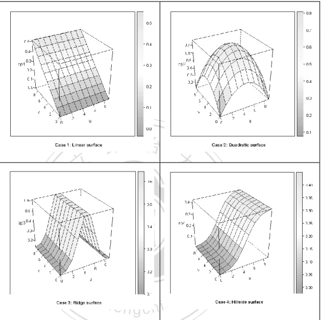
(22) n 1   MSEmethod  i. Average Discount rate:. (13). n 1   MSEOLS  i. where MSE refers to the mean squares error, or the squared root of (bias) 2 plus variance. Note that (13) uses the MSE of the estimate from OLS as a bench mark. Furthermore, (13) can be computed for all locations and we can use the weighted mean of the discount rate for comparisons,.  (MSE. ). OLS location i. i.   MSEmethod / MSEOLS location i .  (MSE. ). .. (14). OLS location i. i. 政治大. Moreover, we can also define other evaluation indices:. 立 Average bandwidth:. n 1   bandwidthmethod . ‧ 國. (15). 學. i.   . Average Variance: n1  Var îk. (16). ‧. i. . y.   2. (17). io. sit. Nat. Average Bias: n 1   îk  ik i . n. al. er. The above evaluation indices allow us to check the accuracy and precision of the. Ch. i n U. v. estimators individually. In general, a good estimator should have small variance, bias and MSE.. engchi. 4.1 Simulation Setting: As mentioned above, there were four types of surfaces for the coefficients (Figure 1). Cases 1 and 2 were polynomial functions (close to linear functions) of the independent variables, and cases 3 and 4 were nonlinear functions. Similar settings also appeared in previous studies on GWR, and they have practical meanings. For example, the quadratic surface (Case 2) often occurs in situations involving housing prices, where prices are significantly higher for locations near a town centre or transportation centre. For example, the relationship between the 16.

(23) size of a house and its price is more obvious in downtown areas than in the countryside. Non- linear surfaces can be used to determine the relationship between floor space and price for both industrial and commercial areas. For every non-stationary surface, we assume that there are 10 by 10 regular lattice points (100 locations). For the fixed effect model, two major scenarios are tested under different S/N ratio. The first scenario is single type surfaces. In this scenario, both intercept and independent variables are composed by same surface, and all four types of aforementioned surfaces will be considered. The second scenario, i.e., mixed type. 政治大. surfaces, is more realistic and assumes that intercept and independent variables. 立. follow different surfaces. We examine the second scenario with two cases, linear-. ‧ 國. 學. quadratic (polynomial surface) and ridge- hillside (non-polynomial surface).. ‧. To ensure the randomness of the experiment and prevent the nuisance effect. sit. y. Nat. caused by specific pattern, the independent variable at each location is drawn. io. al. er. from a uniform distribution on the interval (0, 1) and is fixed for all 100 simulation runs. We consider various values for the independent variable and the. n. iv n C results are very consistent. h To simply the discussion, we will choose only one of engchi U the results as a demonstration. For both models, the errors are drawn from a normal distribution with a mean of 0 and a standard deviation of 0.5. Also, the reason for choosing the standard deviation 0.5 is to incorporate the values of the S/N ratio. However, in the real scenario, the dependent variables are often random due to measurement errors. Moreover, performing the simulation under different dependent variable sets can make the results carry more conviction. Hence, we redo the single-type surfaces simulations under the random effect model, which. 17.

(24) the dependent variable set is drawn repeatedly from uniform distribution on the interval (0, 1) at each sample.. 立. 政治大. ‧. ‧ 國. 學. n. er. io. sit. y. Nat. al. Ch. engchi. i n U. v. Figure 1: Four coefficient surfaces. Cases 1 & 2 are polynomial surfaces and Cases 3 & 4 are non polynomial surfaces.. For the CGWR, the Gaussian kernel is chosen and the optimal bandwidth is the one with the minimum cross- validated sum of squares (CVSS). Furthermore, we require that the bandwidth is within a reasonable range, to prevent the estimation from being too localized or globalized, for extremely small or large bandwidths, respectively. The upper bound of the range is the maximum length on the map and the lower bound is to have at least 5 data points (each with 1/5 of the 18.

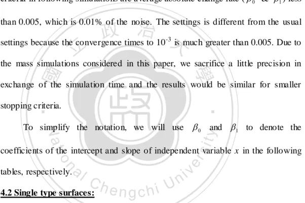
(25) weight). The preceding setting is also used in the “spgwr” package (Bivard and Yu, 2010, ver0.5-4) in R, a free statistical software. The rest of this section discusses the simulation results for the single type surfaces, followed by those for the mixed type surfaces, and finally the random effect models. Specifically, we will compare the performances of three GWR estimations based on the average discount rate, the average bandwidth and the average variance and average bias of the estimates. In addition, the stopping criteria in following simulations are average absolute change rate (  0 & 1 ) less. 治政 settings because the convergence times to 10 大 is much greater than 0.005. Due to 立. than 0.005, which is 0.01% of the noise. The settings is different from the usual -3. the mass simulations considered in this paper, we sacrifice a little precision in. ‧ 國. 學. exchange of the simulation time and the results would be similar for smaller. ‧. stopping criteria..  0 and 1 to denote the. sit. y. Nat. To simplify the notation, we will use. n. al. er. io. coefficients of the intercept and slope of independent variable x in the following tables, respectively.. Ch. 4.2 Single type surfaces:. engchi. i n U. v. Table 1-1 shows the results of the discount rates in the case where B0 and B1 satisfy a linear surface. We can see that both the proposed CGWR and the local linear method have significant improvements over the basic CGWR. Interestingly, the local linear method is better (with respect to smaller discount rates) than the GWR when the S/N ratio is large, but the basic GWR is better when the S/N is small. The reason might be that larger noises produce larger fluctuations, and thus the average tangent line in the local linear method is not accurate or stable. Similar patterns also appear for the other three surfaces (Tables. 19.

(26) 1-2, 1-3, 1-4). This suggests that the local linear method is not very stable if the S/N ratio is small. The CGWR and the local linear method again outperform the basic GWR in the case of a quadratic surface. However, the CGWR appears to be the best and the edge is more obvious when the S/N increased. For the nonlinear surfaces, the CGWR continues to work satisfactorily, but the local linear model does not. It is possible to create worse results than the basic GWR. The CGWR is still reliable in the cases of nonlinear surfaces, performing much better than the other two methods.. 治政 Table 1-1. The average discount rates on a linear surface大 (single-type) 立 B0 0.312. 0.158. 3. 1.348. 0.321. 0.173. 5. 1.775. 0.382. 0.199. 1. 1.317. 0.192. 0.078. 3. 1.107. 0.164. 0.069. a 1 l. 1.299. 0.188. 0.059. Nat. io. n. 5. CGW R. 3 5. v 0.082 i n C h0.664 0.195 U 0.880 e n g0.202 c h i 0.086 0.899. 0.227. 0.092. 3. 5. 1.815. 1.589. 1.328. 0.598. 0.663. 0.755. 0.329. 0.397. 0.459. 2.111. 1.033. 0.686. 0.403. 0.347. 0.284. 0.197. 0.179. 0.126. 1.076. 0.775. 0.412. 0.400. 0.366. 0.286. 0.198. 0.207. 0.178. y. 1.064. 1. sit. 1. er. ‧ 國. 5. ‧. 3. B1. Basic GW R. Local-Linear. 1. 學. B0. B1. Table 1-2. The average discount rates on a quadratic surface (single-type) B0 B0. B1. 1. 3. 5. 1. 3. 5. 1. 1.955. 0.791. 0.510. 2.877. 7.729. 7.542. 3. 3.217. 0.896. 0.570. 1.418. 2.332. 3.650. 5. 4.334. 1.108. 0.639. 0.844. 1.316. 1.819. 1. 3.279. 0.914. 0.535. 5.159. 8.900. 7.941. 3. 5.177. 1.119. 0.599. 2.039. 2.634. 3.481. 5. 6.147. 1.196. 0.602. 1.001. 1.169. 1.488. 1. 1.168. 0.324. 0.146. 1.529. 1.612. 0.928. B1. Basic GW R. Local-Linear. 20.

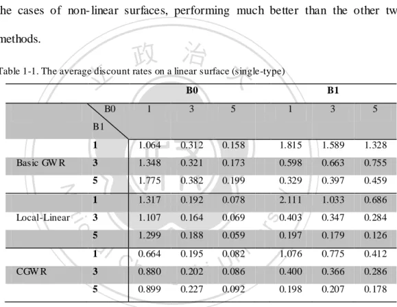
(27) CGW R. 3. 1.491. 0.380. 0.166. 0.675. 0.713. 0.730. 5. 1.709. 0.429. 0.183. 0.374. 0.451. 0.430. Table 1-3. The average discount rates on a ridge surface (single-type) B0 B0. 1. 3. B1 5. 1. 3. 5. B1. Basic GW R. 1. 1.740. 0.571. 0.383. 2.642. 2.325. 2.249. 3. 2.623. 0.728. 0.401. 1.150. 1.375. 1.321. 2.892 0.824 0.433 治政 2.890 1.023 0.621 大 4.340 1.206 0.618. 0.591. 0.810. 0.894. 4.745. 4.374. 3.672. 1.960. 2.255. 2.023. 1.081. 1.326. 1.344. 1.029. 0.428. 0.258. 5 1. 立. 3. CGW R. 5. 5.385. 1.386. 0.677. 1. 0.884. 0.203. 0.111. 3. 1.048. 0.239. 0.116. 0.529. 0.385. 0.250. 5. 0.854. 0.221. 0.107. 0.253. 0.208. 0.159. 學. Nat. y. ‧. ‧ 國. Local-Linear. 1. n. a B0 l. 1. Local-Linear. CGW R. Ch. 3. 5. er. io. B0. B1. Basic GW R. sit. Table 1-4. The average discount rates on a hillside surface (single-type). iv. n e n g c0.315 h i U0.153. 1.075. 1. B1 3. 5. 1.697. 1.905. 1.359. 3. 1.353. 0.340. 0.173. 0.583. 0.603. 0.668. 5. 1.152. 0.343. 0.185. 0.234. 0.278. 0.360. 1. 1.339. 0.243. 0.149. 2.187. 1.549. 1.239. 3. 1.403. 0.289. 0.188. 0.617. 0.529. 0.722. 5. 1.113. 0.339. 0.209. 0.266. 0.307. 0.421. 1. 0.726. 0.170. 0.077. 1.098. 0.761. 0.473. 3. 0.926. 0.199. 0.079. 0.384. 0.348. 0.239. 5. 0.578. 0.192. 0.079. 0.159. 0.158. 0.140. To further evaluate the performances of the three different GWR methods, we can consider the hillside surface (Table 1-4) and the S/N ratio of B0 = B1 = 5 as a demonstration. We can see that the CGWR produces the best fit and the mean 21.

(28) surface looks almost identical to the true surface (Figures 1 and 2). The edge of the mean surface from the basic GWR is not smooth, which may be due to the fewer observations involved in the estimation, i.e., the edge effect. The mean surface of the local linear method does not look like the shape of a hillside at all, but looks like a linear surface.. 立. M ethod 1: Basic GWR. 政治大 M ethod 2: Local liner estimation. M ethod 3: CGWR. ‧ 國. 學. Figure 2: The B1 mean surface of each estimation method fro m 100 simu lations. The simulation scenario is a hillside, and the S/N ratio of B0 = B1 = 5.. ‧. and second values are the average bandwidths of B0 and B1.. n. S/N. al. Basic. GW R. er. io Method. Linear surface Local. C Linear hengchi U 9.73 4.16 ; 7.24 CGW R. 1. 2.35. 3. 1.46. 10.8. 5. 1.2. 10.34. sit. y. Nat. Table 2. The average bandwidths for linear and hillside surfaces (single-type) For CGW R, the first. i vR nGW Basic. Hillside surface Local Linear. CGW R. 2.25. 9.78. 4.72 ; 7.45. 1.65 ; 2.31. 1.47. 9.01. 1.57 ; 2.80. 1.25 ; 1.47. 1.24. 6.04. 1.25 ; 1.66. Intuitively, we expect that the bandwidth is small if the S/N is large, since distant observations can be very different and cause biased estimation. Basically, all three GWR methods have significant drops in bandwidth if we increase the S/N ratio from 1 to 3. Moreover, the bandwidths in the case of a linear surface should be larger than those of a nonlinear surface under the same S/N ratio, since the surface change is quite homogenous in any direction. 22.

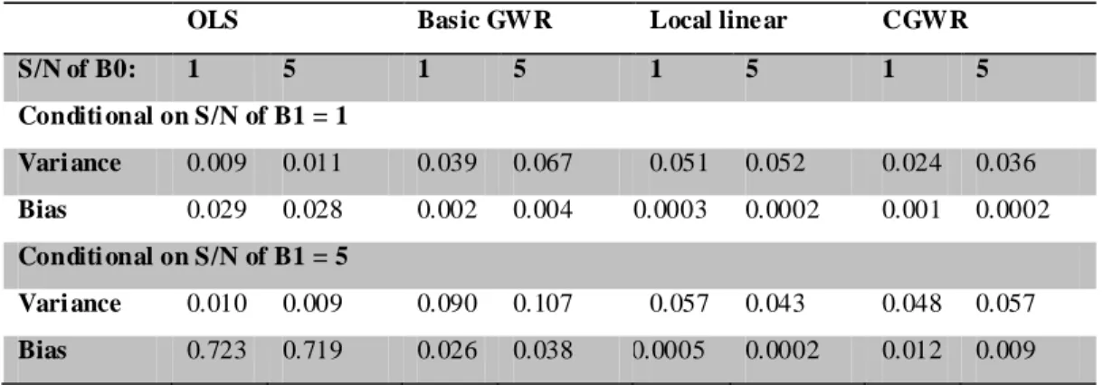
(29) The bandwidth results can also be used to explain why the CGWR outperforms the other two methods. We will choose two surfaces (linear and hillside) to discuss these results (Table 2). The local linear method often yields large optimal bandwidths. If the true surface is close to linear, we can rely on observations within a larger bandwidth and thus ha ve smaller variances than those in the case of a nonlinear surface. Since the shape of a hillside is close to linear, the bandwidths of the hillside case are very similar to those in the linear case (Table 2) and are much larger than those of the quadratic and ridge cases (Appendix B).. 政治大. Furthermore, the values of the CGWR bandwidth match the expected. 立. pattern. For example, if the S/N ratio is small, the bandwidth is expected to be. ‧ 國. 學. large in order to provide a stable estimate. If we fix the S/N ratio of B1, the B0. ‧. bandwidth of CGWR decreases as the S/N ratio of B0 increases, for all four. sit. y. Nat. surfaces (Appendix B). Similar results hold for the B1 bandwidths if we fix the. io. al. er. S/N ratio of B0. This is exactly why we want to consider a different bandwidth for. n. each coefficient, since the numbers of observations needed can be different.. Ch. engchi. i n U. v. Table 3-1. The average variances and biases of B0 and B1 on a linear surface (sin gle-type). (i) B0 OLS S/N of B0:. 1. 5. Basic GWR. Local linear. CGWR. 1. 5. 1. 5. 1. 5. 0.052. 0.024. 0.036. 0.0002. 0.001. 0.0002. 0.043. 0.048. 0.057. 0.0002. 0.012. 0.009. Conditi onal on S/N of B1 = 1 Vari ance. 0.009. 0.011. 0.039. 0.067. 0.051. Bias. 0.029. 0.028. 0.002. 0.004. 0.0003. Conditi onal on S/N of B1 = 5 Vari ance. 0.010. 0.009. 0.090. 0.107. 0.057. Bias. 0.723. 0.719. 0.026. 0.038. 0.0005. 23.

(30) (ii) B1 OLS S/N of B0:. 1. 5. Basic GWR. Local linear. CGWR. 1. 5. 1. 5. 1. 5. Conditi onal on S/N of B1 = 1 Vari ance. 0.031. 0.036. 0.113. 0.190. 0.146. 0.145. 0.071. 0.117. Bias. 0.038. 0.695. 0.013. 0.051. 0.001. 0.0005. 0.004. 0.028. 0.248. 0.294. 0.152. 0.114. 0.088. 0.152. 0.0002. 0.004. 0.010. Conditi onal on S/N of B1 = 5 Vari ance. 0.030. 0.027. Bias. 0.191. 0.880. 立. 政治大 0.048. 0.124. 0.001. S/N of B0:. 1. 5. Basic GWR. Local linear. CGWR. 1. 5. 1. 1. 5. 0.038. 0.044. 0.017. 0.003. 0.006. 0.530. 0.089. 0.084. 0.122. 0.014. 0.018. 5. ‧. Conditi onal on S/N of B1 = 1 0.010. 0.068. 0.152. 0.118. 0.035. 0.049. 0.013. 0.020. 0.011. 0.241. 0.265. 0.487. 0.114. 0.152. Bias. 0.914. a0.010 l C 0.947 h. n. 0.010. engchi. er. io. Conditi onal on S/N of B1 = 5 Vari ance. 0.304. sit. Bias. 0.011. Nat. Vari ance. y. OLS. 學. (i) B0. ‧ 國. Table 3-2. The average variances and biases of B0 and B1 on a ridge surface (single-type). iv 0.091 n U. (ii) B1 OLS S/N of B0:. 1. 5. Basic GWR. Local linear. CGWR. 1. 5. 1. 5. 1. 5. Conditi onal on S/N of B1 = 1 Vari ance. 0.026. 0.033. 0.180. 0.433. 0.333. 0.843. 0.067. 0.188. Bias. 0.049. 0.923. 0.022. 0.136. 0.030. 0.198. 0.011. 0.055. Conditi onal on S/N of B1 = 5 Vari ance. 0.029. 0.029. 0.650. 0.717. 1.302. 1.436. 0.097. 0.178. Bias. 0.377. 1.370. 0.271. 0.541. 0.203. 0.459. 0.008. 0.046. The variances and biases of the estimates from the three GWR methods can also be used for comparisons. Again, we will only use the cases of linear and 24.

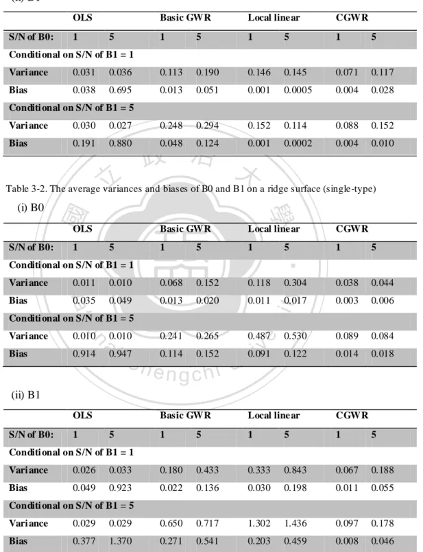
(31) ridge surfaces. Because there are many combinations for the S/N ratios of B0 and B1, we will only show the results of S/N = 1 and 5 (Tables 3-1 to 3-2). Unlike in the previous comparisons, we will also provide the variances and biases of the OLS estimates. In general, a larger S/N ratio tend s to produce a larger bias. Moreover, the OLS estimates fail to capture the spatial trend causing the largest bias, but it uses all of the observations in the estimation (i.e., infinity bandwidth) and thus has the smallest variance. As for the three GWR estimations, the variances of the estimates are generally larger than the biases of the estimates. The results for a linear surface are shown in Table 3-1. As mentioned. 政治大. earlier, the average bandwidths of the local linear method were the largest,. 立. possibly indicating the smallest variances. In addition, the local linear method has. ‧ 國. 學. the smallest bias, and also the smallest discount rates in the case of a linear. ‧. surface (Table 1-1). Although the CGWR has a larger bias than the local linear. sit. y. Nat. method in the case of a linear surface, it dominates the basic GWR with respect to. io. al. er. both variance and bias. The CGWR has the best performance in the case of a ridge. n. surface, and it also outperforms both the basic GWR and the local linear method. i n for both the variance andC bias. hengchi U. v. 4.3 Mixed type surfaces: We also repeat the same comparisons of the three GWR estimation methods with the mixed type surfaces. The results are similar to those in the single type surfaces, and thus we will only show the results of the discount rates. As we mentioned before, there are two cases in this scenario: linear-quadratic (polynomial surface) and ridge- hillside (non-polynomial surface). For the first case, the underlying surface of intercept is linear, and the slope is quadratic. For the second case, all surfaces are of non-polynomial type and it is more complex than the first one. 25.

(32) Table 4-1. The average discount rates of a linear-quadratic surface (mixed-type) B0 B0. 1. 3. B1 5. 1. 3. 5. B1. Basic GW R. Local-Linear. 1. 1.062. 0.279. 0.155. 1.934. 1.643. 1.420. 3. 2.110. 0.407. 0.181. 1.048. 1.067. 0.935. 5. 3.119. 0.537. 0.231. 0.688. 0.687. 0.711. 1. 1.492. 0.225. 0.080. 2.888. 1.514. 0.905. 3.100 0.534 0.169 治政 5.357 0.775 0.268 大. 1.405. 1.314. 0.954. 0.928. 0.871. 0.753. 3 5. 立. 1. 0.183. 0.100. 1.301. 0.802. 0.538. 3. 1.132. 0.345. 0.179. 0.708. 0.849. 0.785. 5. 1.257. 0.388. 0.217. 0.404. 0.523. 0.584. 學. ‧. ‧ 國. CGW R. 0.764. Table 4-2: The average discount rates of a ridge-hillside surface (mixed-type). io. al. n 3 5. Local-Linear. CGW R. y. 3. 5. 1. B1 1. Basic GW R. 1. sit. B0. B1. 1.457. 0.545. er. Nat. B0. 0.337. v ni C h 1.623 0.582 U0.349 e n g c0.604 1.511 h i 0.344. 3. 5. 2.160. 3.268. 2.868. 0.622. 1.373. 1.786. 0.251. 0.586. 0.943. 1. 2.105. 0.853. 0.536. 3.312. 5.602. 4.755. 3. 2.236. 0.903. 0.497. 0.896. 2.348. 2.595. 5. 1.999. 0.980. 0.540. 0.333. 1.076. 1.522. 1. 0.956. 0.245. 0.116. 1.166. 0.750. 0.351. 3. 1.279. 0.361. 0.151. 0.544. 0.677. 0.443. 5. 1.338. 0.485. 0.204. 0.245. 0.434. 0.415. Basically, The CGWR also has smaller discount rates than the basic GWR for the mixed type surfaces (Tables 4-1 to 4-2). We will focus on the results that are different than those of the single type surfaces. Although the local linear estimation is better than the GWR in the linear-quadratic surfaces, it has adverse 26.

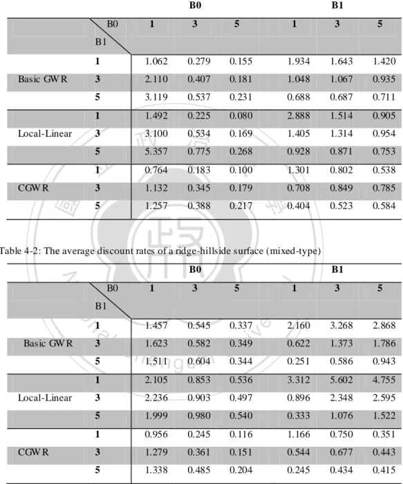
(33) performance in the ridge-hillside surfaces. The results might suggest the instability of local- linear approach. On the contrary, for both cases, the CGWR dominates other two methods, similar to that in the single type scenario. From the computer simulations, we found that the proposed CGWR makes a significant improvement over the basic GWR. If the coefficients surfaces are nonlinear, the CGWR also outperforms the local linear method. In the following section, we will use an empirical example to compare the CGWR and basic GWR, providing further evidence for supporting the CGWR.. 4.4 Random effect model. 立. 政治大. We also repeated the same comparisons of the three GWR estimation. ‧ 國. 學. methods for the random effect model. The results were similar to those for the. ‧. fixed effect model, and thus we will only show the results of the discount rates of. sit. y. Nat. single-type surfaces.. io. B0. n. a B0 l. B1. Basic GW R. Local-Linear. CGW R. er. Table 5-1. The average discount rates on a linear surface (rando m effect).. Ch. 1. 3. engchi. i n U 5. v. B1 1. 3. 5. 1. 0.903. 0.264. 0.134. 1.583. 1.693. 1.493. 3. 1.214. 0.312. 0.159. 0.590. 0.755. 0.794. 5. 1.497. 0.353. 0.169. 0.310. 0.379. 0.426. 1. 0.912. 0.146. 0.049. 1.642. 1.017. 0.601. 3. 0.914. 0.143. 0.053. 0.384. 0.338. 0.271. 5. 0.857. 0.131. 0.052. 0.142. 0.125. 0.111. 1. 0.608. 0.154. 0.067. 0.989. 0.747. 0.355. 3. 0.762. 0.180. 0.085. 0.365. 0.364. 0.283. 5. 0.770. 0.168. 0.079. 0.180. 0.164. 0.164. 27.

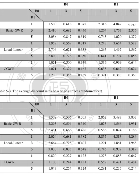
(34) Table5-2: The average discount rates on a quadratic surface (random effect). B0 B0. 1. 3. B1 5. 1. 3. 5. B1. Basic GW R. Local-Linear. 1. 1.500. 0.618. 0.375. 2.316. 4.047. 3. 2.410. 0.682. 0.456. 1.264. 1.767. 1.745 2.376. 5. 3.056. 0.847. 0.519. 0.745. 1.020. 1.379. 1. 1.959. 0.569. 0.317. 3.243. 3.654. 3.522. 3. 2.706. 0.621. 0.338. 1.265. 1.497. 1.562. 0.641. 0.794. 0.856. 1.336. 0.969. 0.644. 0.638. 0.642. 0.624. 0.371. 0.383. 0.363. 5. 立 3 1. 5. 1.071. 0.329. 0.167. 1.230. 0.355. 0.159. 學. ‧. ‧ 國. CGW R. 治 2.800 0.776 0.350 政大 1.021 0.300 0.136. Table 5-3. The average discount rates on a ridge surface (random effect).. n 1. CGW R. 5. 1. B1 3. 5. sit. io. 3a l 5. Local-Linear. 3. B1 1. Basic GW R. 1. 1.508. 0.506. er. Nat. B0. y. B0. 0.305. 2.295 0.594 0.340i v n C h 2.481 0.666 U0.426 engchi 2.020 0.681 0.382. 2.862. 3.497. 3.807. 1.073. 1.566. 1.931. 0.586. 0.824. 1.186. 3.857. 4.313. 4.286. 3. 2.664. 0.778. 0.407. 1.291. 1.861. 1.968. 5. 3.030. 0.835. 0.548. 0.746. 0.937. 1.319. 1. 0.820. 0.227. 0.123. 1.273. 0.883. 0.667. 3. 1.100. 0.244. 0.131. 0.552. 0.471. 0.484. 5. 1.047. 0.254. 0.124. 0.291. 0.275. 0.244. 28.

(35) Table 5-4: The average discount rates on a hillside surface (random effect). B0 B0. B1. 1. 3. 5. 1. 3. 5. 1. 0.969. 0.250. 0.134. 1.624. 1.862. 1.526. 3. 1.238. 0.269. 0.140. 0.545. 0.645. 0.752. 5. 1.356. 0.328. 0.152. 0.307. 0.373. 0.411. 1. 1.021. 0.179. 0.121. 1.797. 1.191. 0.991. 3. 1.202. 0.227. 0.123. 0.535. 0.468. 0.489. 5. 1.100. 0.250. 0.122. 0.245. 0.277. 0.259. 0.913. 0.761. 0.551. 0.359. 0.337. 0.243. 0.189. 0.147. 0.153. B1. Basic GW R. Local-Linear. 1. 立 5. CGW R. 3. 治 0.081 0.620 0.149 政大 0.769 0.165 0.069 0.747. 0.130. 0.070. ‧ 國. 學. The CGWR and local linear estimation also had smaller discount rates. ‧. than the basic GWR for the random effect model (Tables 5-1 to 5-4). We will. y. Nat. io. sit. focus on the results that were different than those of the fixed effect model.. n. al. er. Although the CGWR still dominated in the cases of ridge a nd hillside surfaces,. Ch. i n U. v. the local linear estimation had better performances when the S/N ratio was larger.. engchi. In general, for the random effect model, the local linear estimation was the best in the case of a linear surface, and the CGWR was the best for the other three cases, just as with the fixed effect model. This section showed how computer simulations were used to demonstrate that the proposed CGWR is a significant improvement over the basic GWR. Except for the case of a linear surface, the CGWR also outperformed the local linear method. In the following section, we will show how an empirical study was used to compare the CGWR and basic GWR to provide further evidence to support the CGWR. 29.

(36) Chapter 5. Empirical Study We now apply the CGWR to a real data set. The data considered are from the 2000 Taiwan Population Census and the goal is to study the relationship between elderly disability and related social factors. Like in many developed countries, population aging is a serious problem and the elderly population in Taiwan has increased rapidly. For example, the proportion of people 65 years of age and over was 10.5% in the beginning of 2009, compared to 7% in 1994.. 政治大 northern Taiwan, and this may not match the needs of the elderly. Hu and Yue 立 However, most medical resources are concentrated in metropolitan areas or. ‧ 國. 學. (2002) studied this issue and found that the distribution of elderly disability is spatially autocorrelated and a classic spatial regression model can be applied. Brunsdon. (1999) claimed. that. ‧. However,. the phenomenon of spatial. Nat. sit. y. autocorrelation is likely to be caused by correlated random errors or spatial non-. n. al. er. io. stationarity, (i.e., identifiability). His claim motivates us to re-examine the data using the GWR-based model.. Ch. engchi. i n U. v. The Taiwan census data are at the township level and there are 350 townships involved. The dependent variable is the proportion of disabled elderly people in each township. Since this variable appears to be right skewed, a log * transformation (i.e., yi  log( yi  1) ) is applied. Four independent variables are. selected: population density (POP), proportion of elderly (ELD), higher-age mortality rate (HMR) and education level (EDU). These independent variables are standardized into the interval [0, 1] before being plugging into the GWR model. Before applying the GWR, we first test the spatial non-stationarity (Leung et al., 2000). The F-test of Leung et al. suggests that the model is spatial non-stationary 30.

(37) (p-value < 0.001). This confirms the conjecture of Brunsdon (1999) and we shall continue to proceed with the GWR-type analysis. Table 6. The correlat ions of coefficients from the disability data. The variables INT and POP were in group 1, and ELD, HM R, & EDU were in group 2.. INT. POP. ELD. INT. 1.000. 0.463. -0.949. -0.951. -0.971. POP. 0.463. 1.000. -0.281. -0.281. -0.653. ELD. -0.949. -0.281. 1.000. 0.914. 0.875. HMR. -0.951. -0.281. 0.914. 1.000. 0.868. EDU. -0.971. -0.653. 0.875. 0.868. 1.000. 立. HMR. 政治大. EDU. Since the correlation of intercept and the variable POP is 0.463 (Table 6),. ‧ 國. 學. they are put in the same group. Similarly, the variables ELD, HMR, and EDU are in the other group. Recall that the CGWR does not work well in the case of. ‧. negative correlation. Thus, we focus on the variables with positive correlation and. y. Nat. io. sit. we choose to work on the group of intercept and va riable POP. First, we treat. n. al. er. variable ELD, HMR, EDU as constant, after getting estimates for them from the. Ch. i n U. v. basic GWR. Then, we apply the CGWR to the intercept and the variable POP, as follows:. engchi. ( yi*  îGWR ELDi  îGWR HMRi  îGWR EDUi )  îCGWR  îCGWR POPi  ri 2 3 4 0 1. (18). After fitting the CGWR, the calibrated bandwidths vary across the variables. Here, we let the lower and upper bounds of the bandwidth be (1 km, 400 km). Through the surface after fitting with each method, we find that there is a dramatically different between CGWR and others (Figure 3). For the intercept term, the other methods review the North-South pattern. However, CGWR shows that high disability occurred on inland or mountain area. On the other hand, local. 31.

(38) linear method seems to fit with a linear expansion surface, which is a strong assumption.. We use the pseudo R-square and residual plot to evaluate the performance of CGWR (Figure 4). The pseudo R-square is the Pearson product moment correlation coefficient of the fitted value and the observed value, and a larger value usually indicates a better fit. In this example, the pseudo R-square values of basic GWR and CGWR are 0.514 and 0.894, respectively. Moreover, the residual plots are also in favour of the CGWR, since there are fewer outliers and the. 政治大. outliers appear to have smaller variance.. 立. It should be noted that either one of the variable sets can be chosen as. ‧ 國. 學. constant. If we apply the CGWR procedure on the other variable set (i.e., ELD,. ‧. HMR, and EDU) then the CGWR still has a better fitting result, although the. n. al. er. io. sit. y. Nat. pseudo R-square is 0.874, which is slightly lower.. Ch. engchi. i n U. v. Figure 3: The surface of Intercept and variable POP fro m different fitting method.. 32.

(39) 立. 政治大. ‧ 國. 學. Figure 4: The residual plots & Residual histogram of the GWR,Local linear method and CGW R. (Top) The X-axis shows the fitted values and the Y-axis rep resents their standardized residuals.. ‧. (Bottom) The X-axis shows the residual value.. n. er. io. sit. y. Nat. al. Ch. engchi. i n U. v. 33.

(40) Chapter 6. Discussion and Concluding Remarks Beginning from past decade, the GWR has acted as a new modelling technique used to deal with spatial non-stationarity. This technique allows regression coefficients to vary across space and obtains their estimates from a fixed bandwidth of observations. However, using a fixed bandwidth might not be appropriate since the independent variables would behave differently. In this paper, we proposed a method (CGWR) for modifying the GWR by relaxing the. 政治大 and a local linear estimation, which was shown to be effective at reducing the 立. restriction of a fixed bandwidth. We compared the proposed method to the GWR. ‧ 國. 學. bias. Based on simulation results, we found that the CGWR has the best performances given that the regression coefficients are positively correlated, and. ‧. this advantage is especially noticeable in the cases of non-linear surfaces.. Nat. sit. y. Of course, the improvements in the CGWR are due to the fact that it. n. al. er. io. allows the bandwidth to vary for each coefficient. If the coefficients are positively. i n U. v. correlated, the CGWR can reduce the bias, as well as the variance. In the. Ch. engchi. empirical study, if the coefficients are not always positively correlated, the CGWR can still be modified and applied to a set of variables that are positively correlated for any pairs of variables. However, the proposed method also has limitations. First, the most critical one is probably that the current settings for CGWR do not work well in the case of negative correlation, allowing the basic GWR to outperform the proposed CGWR. As a solution, we suggest calculating the correlation coefficients of the variables before applying the CGWR. Nevertheless, we can perform a two-stage fitting as we did at previous empirical study. In order to verify the feasibility of this approach, we conduct a experiment in two variables. That is, there are three 34.

(41) components in this model, which is intercept and two independent variables. Here, we redo the simulation by fixing second variable at first stage. By ratio of average discount rate, the outcome is similar to previous result. CGWR seems to fit well by this approach. Second, the CGWR is a computer intensive method, and would become extremely time-consuming if there are more variables. To increase the iteration speed, a moving average method could be used to increase the convergence speed. Third, we have not shown that the CGWR will converge if there are many variables, although we found that it would for cases up to four variables. A possible modification to a case with more variables would be to. 政治大. separate the variables into two groups and use double iteration. Then, CGWR. 立. could be used on each group of variables (inner loop ), and the process re- iterated. ‧ 國. 學. between the two groups (outer loop) until both groups of variables converge. To. ‧. show that this idea is feasible, we conduct an experiment with six variables. The. sit. y. Nat. variables are separated into two groups of three variables each, and the estimation. io. n. al. er. does converge.. Ch. engchi. i n U. v. 35.

(42) 政治大 Figure 5: Average discount rate of each method by fixing variab le x2, The baseline of the ratio of 立 average discount rate is the GW R.. ‧ 國. 學. In this study, we also found some potential problems in applying the. ‧. GWR. The GWR still has room for further improvement, especially when the S/N. y. Nat. io. sit. ratio is small, the surfaces of the coefficients are nonlinear and the coefficients. n. al. er. are very different. In addition, the variance reduction of CGWR over GWR is. Ch. i n U. v. much more obvious than that for the bias reduction. This indicates that the GWR. engchi. estimates have large variances. In other words, if the variances of the GWR estimates could be reduced, the bias could also be further reduced, and thus it is likely that the estimates would be more stable.. 36.

(43) References Bivand R, Danlin Y, 2010, R manual for package “spgwr”, http://cran.r-project.org/web/packages/spgwr/spgwr.pdf (2010/08/01) Bivand R, R. Brunstad R, 2005, Further Explorations of Interactions between Agricultural Policy and Regional Growth in Western Europe. Approaches to Nonstationarity in Spatial Econometrics, http://www.feweb.vu.nl/ersa2005/final_papers/671.pdf (2010/09/30) Brunsdon C, Fotheringham A S, Charlton M, 1998, “Geographically weighted regression: modelling spatial nonstationarity” The Statistician 47, 431 – 443. 政治大. Brunsdon C, Fotheringham A S, Charlton M, 1999, “Some notes on parametric. 立. significance tests for geographically weighted regression” Journal o f Regional. ‧ 國. 學. Science 39, 497 – 524. ‧. Brunsdon C, Fotheringham A S, Charlton M, 2002, Geographically Weighted Regression: the analysis of spatially varying relationships (John Wiley &. er. io. sit. y. Nat. Sons). Cleveland W S, Grosse E, Shyu W M, 1991, “ Local regression models”. n. al. Ch. i n U. v. Statistical Models in S (Chambers, J. M. and Hastie,T. J., eds), 309–376.. engchi. (Wadsworth & Brooks, Pacific Grove.) Cressie N, 1993, Statistics for spatial data (John Wiley & Sons) Fan J Q, Zhang W Y, 2008, “ Statistical methods with varying coefficient models” Statistics and its interface 1, 179 – 195 Farber S, Páez A, 2007, “A systematic investigation of cross-validation in GWR model estimation: empirical analysis and Monte Carlo simulations” Journal of Geographical Systems 9, 371 – 396 Haining R, 2003, Spatial data analysis, Theory and practice (Cambridge University Press) 37.

(44) Hastie T J, Tibshirani R J, 1990, Generalized additive models, (Chapman and Hall, London, New York) Hu Y W, Yue J C, 2002, “Spatial Analysis of Taiwan Elderly Disability” Technical Report, Department of Statistics, National Chengchi University, Taipei, Taiwan R.O.C. Leung Y, Mei C L, Zhang W X, 2000, “Statistical tests for spatial nonstationarity based on the geographically weighted regression model” Environment and Planning A 32, 9 – 32 Manoranjan V S, Olmos G M, 1997, “A Two-Step Jacobi-Type Iterative Method”. 政治大. Computers Math. Application 34, 1, 1 – 9. 立. Shi H J, Zhang L J, Liu J G, 2006, “A new spatial-attribute weighting function for. ‧ 國. 學. geographically weighted regression” Canadian Journal of Forest Research 36,. ‧. 4 996 – 1005. sit. y. Nat. Wang N, Mei C L, Yan X D, 2008, “Local linear estimation of spatially varying. io. er. coefficient models: an improvement on the geographically weighted regression technique” Environment and Planning A 40, 986 – 1005. al. n. iv n C Wu C O, Chiang C T, 2000,h“Kernel smoothing e n g c h i Uon varying coefficient models with longitudinal dependent variable” Statistica Sinica 10, 433 – 456. 38.

(45) Appendix A. The outline proof of the convergence for CGWR with fixed bandwidths. Consider a non–stationary model with only the intercept and a single explanatory variable (i.e., yi  fi1  fi2   i ), where  i is random error. To show the convergence of the CGWR algorithm, we first let the initial values be fˆ1 (0)  fˆ2 (0)  0 . Then the estimation of fˆ1 & fˆ2 can be written as: fˆ1 (k )  S1Y  S1S 2Y  S1S 2S1Y  S1S 2S1S 2Y  ...  R1 fˆ (k )  S Y  S S Y  S S S Y  S S S S Y  ...  R. 政治大 are立 the remainder terms of the estimators:. 2. 2 1. 2 1 2. 2 1 2 1. 2. 學. ‧ 國. where R1 & R2. 2. To prove the convergence of the CGWR algorithm, we need to show that both R1 and R2 will converge to 0. Since the discussions of R1 and R2 are. ‧. similar, we will only show the case for R1 .The case for R1 can be separated into. er. io. sit. y. Nat. two parts:. Let (S1S2 )k  P1Bk P , where P is a matrix of eigenvectors for S1S 2 at its *. *. n. al. columns, Bk. *. Ch. engchi. i n U. v. is a diagonal matrix with eigenvalues for S1S 2 on the diagonal,. and k* is an arbitrary natural number. If the largest eigenvalue in the absolute values of S1S 2 ,  , is smaller than 1, then the remainder R1 converges to 0 as k  . . The smoothing matrices in the proof are similar to those used in the GAM. According to Hastie and Tishibirani (1990), the smoother matrices should satisfy the bounded condition (p. 121). Moreover, this assumption seems to be true in practice and it is always the case in our simulation and empirical studies.. 39.

(46) Appendix B. Detailed results for bandwidths (fixed effect models, single-type) Note that the CGWR has two bandwidths for two coefficients, B0 and B1, respectively.. Linear surface B0. Quadratic surface. 1. 3. 5. 1. 3. 5. 1. 2.35. 1.57. 1.35. 4.03. 1.13. 0.98. 3. 1.75. 1.46. 1.26. 1.26. 1.03. 0.94. 5. 1.56. 1.31. 1.20. 1.09. 0.98. 0.92. 1. 9.73. 9.56. 10.26. 2.63. 1.58. 1.22. 3. 10.56. 1.71. 1.33. 1.13. 5. 10.01 立. 1.50. 1.21. 1.06. 6.58 ;7.77. 0.87 ; 8.27. 0.66 ; 6.28. B1. Linear. 1.60 ; 4.82. 1.23 ; 5.19. 3. 4.23 ; 2.70. 1.65 ; 2.31. 1.18 ; 2.28. 6.02 ; 3.69. 0.82 ; 3.82. 0.61 ; 2.10. 5. 3.50 ; 1.70. 1.60 ; 1.65. 1.25 ; 1.47. 4.77 ; 1.44. 0.89 ; 1.35. 0.61 ; 0.88. 0.83. 3. 1.16. 0.89. 0.77. 5. 1.01. 0.80. 0.73. 2.61. 1.33. 1.03. 1.12. i n U. al. n. Linear. CGW R. io. 3. Ch. 1.68. e n1.01 gchi. Hillside surface. 2.25. 1.67. 1.41. y. 1.01. Nat. 4.2. 1 Local-. ‧. Ri dge surface. 1. GW R. 學. CGW R. 4.16 ; 7.24. ‧ 國. 1. 政 10.8 治 10.06 大 9.82 10.34. 1.79. 1.47. 1.31. sit. Local-. 1.63. 1.43. 1.24. 9.78. 9.78. 8.2. 9.75. 9.01. 7.4. 0.91. 8.67. 8.93. 6.04. 0.95. er. GW R. v. 5. 1.28. 1. 4.79 ; 8.79. 0.85 ; 8.69. 0.65 ; 5.45. 4.72 ; 7.45. 1.63 ; 5.83. 1.25 ; 5.34. 3. 5.24 ; 4.07. 0.83 ; 2.15. 0.66 ; 1.12. 4.98 ; 3.11. 1.57 ; 2.80. 1.24 ; 2.70. 5. 3.64 ; 1.16. 0.80 ; 0.99. 0.65 ; 0.79. 5.09 ; 1.67. 1.68 ; 1.64. 1.25 ; 1.66. 40.

(47)