chains well entangled in polymer melts
Y.-H. Lin and C.-F. Huang
Citation: The Journal of Chemical Physics 128, 224903 (2008); doi: 10.1063/1.2927870 View online: http://dx.doi.org/10.1063/1.2927870
View Table of Contents: http://scitation.aip.org/content/aip/journal/jcp/128/22?ver=pdfcov Published by the AIP Publishing
Articles you may be interested in
A single particle model to simulate the dynamics of entangled polymer melts J. Chem. Phys. 127, 134901 (2007); 10.1063/1.2780151
Coarse grained model of entangled polymer melts J. Chem. Phys. 125, 164907 (2006); 10.1063/1.2362820 The dynamics of single chains within a model polymer melt J. Chem. Phys. 122, 114902 (2005); 10.1063/1.1863852
Recirculation cell for the small-angle neutron scattering investigation of polymer melts in flow Rev. Sci. Instrum. 74, 4052 (2003); 10.1063/1.1602939
Linear rheology of binary melts from a phenomenological tube model of entangled polymers J. Rheol. 46, 671 (2002); 10.1122/1.1459445
The Rouse–Mooney model for coherent quasielastic neutron scatterings
of single chains well entangled in polymer melts
Y.-H. Lina兲and C.-F. Huang
Department of Applied Chemistry, National Chiao Tung University, Hsinchu, Taiwan 30050
共Received 18 February 2008; accepted 22 April 2008; published online 9 June 2008兲
The dynamic structure factor共DSF兲 for single 共labeled兲 chains well entangled in polymer melts has been developed based on the Rouse–Mooney picture; the DSF functions derived from the Langevin equations of the model in both discrete and continuous forms are given. It is shown that for all practical purposes, it is sufficient to use the continuous form to analyze experimental results in the “safe” q region 共q being the magnitude of the scattering wave vector q兲 where the Rouse-segment-based theories are applicable. The DSF form reduces to the same limiting form as that of the free Rouse chain as q2a2or q2R2→⬁ 共a and R being the entanglement distance and the
root mean square end-to-end distance, respectively兲, confirming what has been expected physically. The natural reduction to the limiting form allows the full range of DSF curves to be displayed in terms of the reduced Rouse variable q2共Z
dt兲0.5in a unified way. The displayed full range represents
a framework or “map,” with respect to which effects occurring in different regions of the DSF may be located and studied in a consistent manner. One effect is the significant or noticeable deviations of the theoretical DSF curves from the limiting curve in the region⬃4⬎q2共Z
dt兲0.5⬎ ⬃0.1 共a time
region where t⬍1
e兲 to the faster side as qa is in the range 1–5. This is supported by the comparison
of the experimental results of an entangled poly共vinylethylene兲 sample with the theoretical curves. The DSF functional forms predict plateaus with heights depending on the value of q—q-split plateaus—as can be experimentally observed in the time region greater than the relaxation time1e of the lowest Rouse–Mooney mode, when qa falls between ⬃1 and ⬃7. High sensitivity of the distribution of the q-split plateaus to a enables its value to be extracted from matching the calculated with the experimental results. The thus obtained a value for a well-entangled poly共ethylene-co-butene兲 polymer is in close agreement with the rheological result. It is shown that the fixed-end boundary conditions in the Rouse–Mooney model are responsible for the correct prediction of the distribution of the q-split plateaus. © 2008 American Institute of Physics. 关DOI:10.1063/1.2927870兴
I. INTRODUCTION
Because of the large number of atoms and degrees of freedom in a chain molecule, a polymer is rich in its dynam-ics, with its relaxation-time distribution covering many decades.1–5Various techniques have been used to study dif-ferent aspects of polymer dynamics. In comparison with the wide range that the viscoelastic-response measurements are capable of probing, the neutron spin-echo spectroscopy for studying the coherent scattering has a narrower time window and is mainly suitable for probing certain aspects of chain dynamics.6Successful models have been developed describ-ing the viscoelastic responses quantitatively over the whole range: From the glassy-relaxation region to the flow region.7–9The physical pictures as contained in these models may provide the approaches for analyzing the coherent quasielastic共or dynamic兲 neutron scattering results.
The relaxation modulus G共t兲 functional forms have been given7–9 by incorporating a stretched exponential Kohl-rausch, Williams, and Watts 共KWW兲 form for the glassy-relaxation process G共t兲 into the extended reptation
theory2,10–12 共ERT兲 共for entangled systems兲 or the Rouse theory2,13–16共for entanglement-free systems兲 as the frame of reference. The creep compliance J共t兲 curves17–19 and vis-coelastic spectra G*共兲 共Ref. 20兲 of nearly monodisperse
polystyrene melts have been recently7–9 quantitatively ana-lyzed over the whole range in terms of the G共t兲 functional forms. From the extensive J共t兲 and G*共兲 line-shape
analy-ses, it is clear that the Rouse modes of motion R共t兲 is the
only dynamic process following the glassy-relaxation pro-cessG共t兲 in an entanglement-free system. As entanglements
begin to occur with increasing molecular weight, R共t兲 is
replaced by the Rouse–Mooney modes of motion2,10–12,21
A共t兲—modes of motion of an entanglement strand with both
ends fixed—as the first process right after G共t兲. The A共t兲
process plays an important role in the success of the ERT, quantitatively describing the transition from the glassy-relaxation region to the rubberlike-to-fluid region—the
X共t兲−B共t兲−C共t兲 region 2,7–12
—in the relaxation modulus G共t兲.
Concurrently, dynamic neutron scatterings from single 共labeled兲 entanglement-free chains in polymer melts are well described by the Rouse model, if the magnitude of the scat-tering wave vector q is not too large6,22 共q艋 ⬃1.5 nm−1 or
a兲Electronic mail: [email protected].
0021-9606/2008/128共22兲/224903/12/$23.00 128, 224903-1 © 2008 American Institute of Physics This article is copyrighted as indicated in the article. Reuse of AIP content is subject to the terms at: http://scitation.aip.org/termsconditions. Downloaded to IP:
qb艋 ⬃2, with b being the typical root mean square length of a Rouse segment, b =具b2典0.5 for the studied polymers兲. For
q⬎ ⬃1.5 nm−1, deviations from the Rouse theory may be
due to the segmental interactions within and between “Rouse” segments.23 In well-entangled systems, the single-chain dynamic scatterings deviate in a characteristic way from being described by the Rouse model even in the q艋 ⬃1.5 nm−1region. The understandings gained from the
stud-ies of the viscoelastic responses G共t兲, J共t兲, and G*共兲 共Refs.
2 and 7–12兲 suggest that dynamic scatterings from well-entangled labeled chains may be studied in terms of the Rouse–Mooney model. Restricted to the length scale of an entanglement strand, a, the “static” 共“structural”兲 and dy-namic properties revealed by the scatterings are expected to be independent of molecular weight. Indeed, experimental results24 have suggested that the dynamic-scattering line shapes become independent of molecular weight if the molecular weight is sufficiently large—i.e., if the polymer system is extremely well entangled.
II. DYNAMIC STRUCTURE FACTORS OF ROUSE-SEGMENT-BASED MODELS A. Free chains
The Rouse dynamic behavior is described by the Lange-vin equation1,2,25 for a chain consisting of beads connected by springs with the entropic-force constant 3kT/b2.1,2,13,14
Consider a single Rouse chain—labeled in experimental measurements—with N0beads, whose positions at time t are denoted by 兵Rn共t兲其. With the beads’ displacements being
sums of Gaussian random steps, the dynamic structure factor 共DSF兲 of the single Rouse chain can be expressed by1,6
S共q,t兲 = 1 N0n=1
兺
N0兺
m=1 N0 具exp关iq · 共Rm共t兲 − Rn共0兲兲兴典 = 1 N0n=1兺
N0兺
m=1 N0 exp冋
−q 2 6 具共Rm共t兲 − Rn共0兲兲 2典册
. 共1兲In terms of the Rouse normal modes,1,2 while the DSF de-rived from Eq. 共1兲 based on the discrete model is given in Appendix A, the one based on the continuous model is given by1,6 S共q,t兲 = 1 N0 exp共− q2D Gt兲 ⫻
兺
n=1 N0兺
m=1 N0 exp冋
−q 2 6 b 2兩m − n兩 −2q 2N 0b2 32 p=1兺
⬁ 1 p2cos冉
mp N0冊
cos冉
np N0冊
⫻冋
1 − exp冉
− t p冊
册
册
, 共2兲 with p= N02b2 3kT2p2= K M2 3p2. 共3兲In Eq. 共3兲, M is the molecular weight corresponding to N0 beads per chain, and the frictional factor K is given by共see Appendix B兲 K = b 2 kT2m2= K⬁2 kT2b2= 3K⬁2 2Z d , 共4兲
with m being the mass per Rouse segment. As explained in Appendix B, the frictional factor K serves an equivalent role as the parameter Zd 共=3kTb2/兲 that has often been used to
characterize the dynamic neutron scatterings and will be used in the data analyses below.
If the free Rouse chain is trapped inside a domain with a diameter of
冑
N0b, the DSF is obtained from Eq. 共2兲 bysetting DG= 0: S共q,t兲 = 1 N0 ⫻
兺
n=1 N0兺
m=1 N0 exp冋
−q 2 6b 2兩m − n兩 −2q 2N 0b2 32兺
p=1 ⬁ 1 p2cos冉
mp N0冊
cos冉
np N0冊
⫻冋
1 − exp冉
− t p冊
册
册
. 共5兲Eq. 共5兲will be used in Sec. VI.
B. Entanglement strands
Here, we consider an extremely well-entangled system in which both the labeled chains and the matrix chains are very long with molecular weights much greater than the entangle-ment molecular weight Me. In other words, N = N0/NeⰇ1,
with N0 denoting the number of Rouse segments of a chain
and Nedenoting the number of Rouse segments per
entangle-ment strand. Consider an entangleentangle-ment strand of a labeled chain in the system. We picture that the first bead R1共t兲 is
connected to the fixed origin O of a chosen coordinate sys-tem by a bond vector b0共t兲 and the last bead RNe共t兲 is fixed at
such a position Rethat statistically具Re 2典=N
eb2= a2, where a
is referred to as the entanglement distance or length. En-tanglement strands are linked one after another, each with its end-to-end vector Rerandomly oriented.1,2,26If the
represen-tative entanglement strand defined above stands for a par-ticular one in the sequence, the origin O is equivalent to the position of the last bead of the preceding entanglement stand and RNe共t兲 is equivalent to the origin of the next
entangle-ment strand. In this way, beads on each entangleentangle-ment strand of a chain are counted in an equivalent manner.
As NⰇ1, in the timescales as typically probed by the neutron spin-echo spectroscopy—with a properly chosen temperature—entanglement points may be regarded as fixed as the chain does not have the chance to slip through the links共the slip links of the Doi–Edwards model1,2,26兲. Then as shown in Appendix C, under the condition RⰇq−1, the DSF of the labeled chain can be expressed as
S共q,t兲 = 1 Ne
兺
n=1 Ne兺
m=1 Ne 具exp关iq · 共Rn共t兲 − Rm共0兲兲兴典 = 1 Ne兺
n=1 Ne兺
m=1 Ne exp冋
−q 2 6具共Rm共t兲 − Rn共0兲兲 2典册
, 共6兲where the Gaussian property of the beads’ movements has been used. Although the term with n = m = Nein Eq.共6兲being
independent of time does not represent a Gaussian dynamic process, with respect to it, the second equality in Eq. 共6兲 remains valid.
Equation共6兲 is referred to as the Rouse–Mooney model of coherent quasielastic scattering. In terms of the normal modes,2,27while the DSF derived from Eq.共6兲based on the discrete model is given in Appendix A, the one based on the continuous model is given by
S共q,t兲 = 1 Ne ⫻
兺
n=1 Ne兺
m=1 Ne exp冋
−q 2 6b 2兩m − n兩 −2q 2N eb2 32兺
p=1 ⬁ 1 p2 sin冉
mp Ne冊
sin冉
np Ne冊
⫻冋
1 − exp冉
− t p e冊
册
册
, 共7兲 with p e = Ne 2b2 3kT2p2= K Me2 3p2. 共8兲There are two main differences between Eqs.共2兲and共7兲 in form: First, the diffusion factor is absent from Eq. 共7兲, reflecting that the chain does not diffuse due to the entangle-ment points being fixed as assumed. Second, because of the changes in the boundary conditions, cosines in Eq. 共2兲 关or Eq.共5兲兴 are replaced by sines in Eq.共7兲共taking N0as
corre-sponding to Ne兲. While the diffusion motion does not occur
in either Eq. 共5兲 or 共7兲, the former is for a chain with both ends free while the latter is for a strand with both ends fixed. As explained in Appendix D, for q2N
eb2Ⰷ1, Eq. 共7兲 in the
short-time region 共tⰆ1e兲 reduces to the same limiting form 关Eq.共D3兲兴 as the one that is obtained from Eq.共2兲or共5兲for
q2N
0b2Ⰷ1 in the equivalent way.
One may obtain the self-correlation function—as can be probed by incoherent scattering—from Eq. 共7兲 by setting n = m. In the time region tⰆ1e, the exponent is dominated by the terms with large p. By replacing sin2共np/Ne兲 by the
average12 and converting the summation over p into integra-tion, one obtains
Sself共q,t兲 = exp
冋
− q2Neb2 32冕
0 ⬁ 1 p2冋
1 − exp冉
− tp2 1 e冊
册
dp册
= exp冋
−冉
tZdq 4 9冊
1/2册
. 共9兲 Equation 共9兲 is identical to the one that is obtained from Eq.共2兲for the time region tⰆ1in the equivalent way1,6—inthe case of from Eq. 共2兲, replacing cos2共np/N0兲 by the
average 12. Thus, even though in the literature the equation 关Eq.共9兲兴 used to analyze the short-time incoherent scattering data of entangled systems has been understood共or regarded兲 as originating from the Rouse theory关Eq.共2兲兴,6the analysis-obtained results are equally applicable here—i.e., from the perspective of the Rouse–Mooney model.
III. APPLICABLE q REGION FOR ROUSE-SEGMENT-BASED THEORIES
Before we analyze experimental results in terms of the Rouse and Rouse–Mooney models given above, it is advis-able to point out some recent developments in the under-standing and characterization of the Rouse or “Rouse” seg-ment based on Monte Carlo simulations on entangleseg-ment- entanglement-free Fraenkel chains.28,29 It has been concluded that the entropic-force constant on each segment is not a required element to give rise to the Rouse modes of motion in G共t兲 of an entanglement-free system. As the Fraenkel segment with a sufficiently large force constant can be regarded as basically equivalent to the Kuhn segment as far as the chain confor-mation is concerned, this conclusion has provided an expla-nation resolving the paradox that the molecular weights of the Rouse segments and Kuhn segments, m and MK, are of
the same order of magnitude.30 Thus, the “Rouse” segment having a finite size can be determined experimentally—in general much greater than a chemical segment; for instance, m = 850 for polystyrene and m = 200– 260 for polyisobutylene,30–32 the entropic共rubbery兲 aspects of poly-mer viscoelasticity in reality are not directly related to the entropic-force constant of the Rouse segment. In spite of this, the Rouse-segment-based molecular theories can still be profitably used in analyzing experimental results. The wide use of the Rouse-segment-based molecular viscoelastic theo-ries can be attributed to two main reasons: One is that their equations of motion are solvable analytically1,2,10,13,14 and the other is the success of the theories in interpreting experi-mental results—over the entropic region of viscoelastic re-sponse. Here, we take a similar practical view of using the Rouse-segment-based DSF functional forms given in this re-port. Because the “Rouse” segment has a finite size, the Zd
values, although still extractable from analyses in terms of these DSF functional forms, will eventually cease to be in-dependent of q when q is sufficiently large. Thus, for safe use of the DSF functional forms, one needs to adhere to the criterion that the Zd values extracted from the experimental
DSF data at different q values are in agreement with each other.
In Fig. 1, DSF curves of an entanglement-free poly-isobutylene 共PIB兲 sample 关Mn= 3870 and Mw/Mn= 1.05
共Ref. 22兲兴 at different q values are compared to the results calculated by substituting N0= 15 and b = 1.255共Ref.30兲 into
Eq. 共A1兲 and by substituting N0= 200 and b = 0.3323 into
Eq. 共2兲—the values of the N0 and b are chosen such that
R2= K
⬁M = N0b2= 22.06 nm2 is maintained.2,22,33 Failure of
the Rouse model at large q being expected, in the compari-son between theory and experiment, a Zdvalue is chosen by
matching the calculated and measured curves at as many low q values as possible. The close matching between theory and This article is copyrighted as indicated in the article. Reuse of AIP content is subject to the terms at: http://scitation.aip.org/termsconditions. Downloaded to IP:
experiment at the q⬍1.5 nm−1region with a small difference
at q = 1.5 nm−1 is made with the same Z
d value
共0.808 nm4/ns兲 as used by Richter et al.22
In the q艋1.5 nm−1 region, the curves calculated from Eqs. 共A1兲
and Eq.共2兲agree well with each other. Thus, for all practical purposes, the continuous model may be used for comparison with the experimental results in the region q艋1.5. This re-gion may be regarded as the applicable or safe rere-gion of the Rouse theory. The justification for using the continuous Rouse model in the safe q region does not mean that the chain section that can be assigned as a Rouse or “Rouse” segment is very small. The N0and b values chosen for
sub-stituting into Eq. 共2兲 are merely some convenient numbers arbitrarily chosen共also see Appendix B兲. We have found that as long as R2= N0b2is maintained, virtually no difference can
be observed between the calculated DSF curves with differ-ent N0 values greater than 50 except at large q values 共3.0 and 4.0 nm−1兲. The above discussion also confirms the
prac-tice in the literature where the continuous form has always been used in analyzing neutron spin-echo data in the safe q region.
Equations共2兲and共7兲 are both developed from the same basis using the Rouse segment as the basic structural unit. The Rouse segment lengths b estimated for the polymers studied in this paper are of the same order of magnitude 共1.25–1.4 nm兲. Thus, the region q艋 ⬃1.5 nm−1, where
suc-cessful comparison between Eq.共2兲and experiment is made in Fig.1, can also be regarded as the safe q region for evalu-ating the success of Eq.共7兲. All the analyses done below for the entangled systems, except for the result of the poly共vinylethylene兲 共PVE兲 sample at q=1.79 nm−1, basically
fall in the safe region. Although small differences between Eqs. 共A5兲 and 共7兲 can be noticed in the calculated curves 关over the plateau region for the poly共ethylene-co-butene兲 共PEB-2兲 system studied below兴, the differences are much smaller than the noise of the data.
IV. ENTANGLEMENT-RELATED CHARACTERISTICS IN THE DSF LINE SHAPES
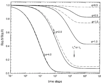
Equation 共7兲 gives rise to unique DSF line shapes be-cause of the existence of entanglement with a characteristic length a. When the scattering wave vector q is of such mag-nitude that⬃10⬎qa⬎ ⬃1, two characteristics can be iden-tified in the DSF line shapes, as shown in Fig.2. One occurs in the time region, t⬎1e; the other in the t⬍1e region. By emphasizing these characteristics in analyzing the experi-mental results in terms of Eq.共7兲, one may effectively extract the value of a. To illustrate these two characteristics in perspective, the DSF line shapes calculated from Eq. 共7兲 at q = 0.5, 1, and 2 and shown in Fig.2are displayed in Fig.3 as a function of the reduced Rouse variable q2共Z
dt兲1/2.
As shown in Appendix D, under the condition qaⰇ1, Eq.共7兲in the time region tⰆ1ereduces to the limiting form, Eq. 共D3兲,1,34 which is a universal function of the reduced variable q2共Z
dt兲1/2. As the condition is changed from
qa⬎10 to qa⬎1, obvious plateaus occur in the time region t⬎1e, whose heights depend on the value of qa. The way that the q-split plateaus are distributed is sensitive to the value of a—as indicated by S共q,tⰇ1
e兲/S共q,0兲=0.83 at
qa = 2.5 vs S共q,tⰇ1
e兲/S共q,0兲=0.075 at qa=10. This unique
relationship enables the entanglement distance a to be ob-tained from matching the calculated and measured plateau heights at different q values simultaneously.
The other characteristic occurring in the region t⬍1eis relatively subtle, requiring some careful explanations. As shown in Fig.3, the DSF at q = 0.5 or qa = 2.5 deviates in the region of ⬃3⬎q2共Zdt兲0.5⬎ ⬃0.2 from the limiting form
关Eq. 共D3兲兴 to the faster side. Similarly significant or notice-able deviations occur as qa falls between ⬃1 and ⬃5; here, we use the deviation at qa = 2.5 as a representative case for explanation.
Imagine an “experimental” system of very high molecu-lar weight, where entanglements could be “switched on and FIG. 1. Comparison of the measured normalized DSF results共䊊, 쎲, 䉭, 䉱,
䊐, 䊏, 〫, and ⽧ at q=0.4, 0.6, 0.8, 1.0, 1.5, 2.0, 3.0, and 4.0 nm−1,
respec-tively兲 of the PIB sample with the curves calculated from the Rouse model: 共—兲 from the discrete form, Eq.共A1兲共with N0= 15 and b = 1.255 nm, giving
R2= 22.06 nm2兲; 共---兲 from the continuous form, Eq. 共2兲 共with N 0= 200
and b = 0.3323 nm, giving R2= 22.06 nm2兲. The comparison is made with
Zd= 0.808 nm4ns−1; the arrow marks the position of1.
FIG. 2. Normalized DSF curves calculated from Eq.共7兲for entanglement strands共both ends fixed; with Ne= 100 and b = 0.5, giving a = 5兲 are shown as
solid lines at the indicated q values. For comparison, the corresponding curves calculated from Eq. 共5兲for free chains共with N0= 100 and b = 0.5兲
trapped in a domain of diameter a = 5 are shown as dashed lines. The arrow marks the position of1e关for Eq.共7兲兴 or
1关for Eq.共5兲兴.
off:” If entanglement is on, the system is extremely well entangled—thus, both ends of each entanglement strand can be assumed as fixed—and its entanglement distance a is as-sumed such that qa = 2.5. If entanglement is off, the dynamic behavior of the system is described by the Rouse theory un-der the condition qRⰇ1. In the entanglement-free situation, because qRⰇ1, the DSF over the short-time region is well described by Eq.共D3兲. As entanglement is switched on, due to the imposition of the condition qa = 2.5, the above de-scribed deviation from Eq.共D3兲shows up. Such a deviation is expected to be observed by monitoring the apparent Zd
values that can be extracted from comparing the experimen-tal curves at qa = 2.5 with Eq.共D3兲. In the entanglement-free situation, the apparent Zdvalues at different q values should
be the same as qRⰇ1 in all cases. In comparison, the appar-ent Zdvalue in the entangled situation should be larger due to
the deviation from Eq. 共D3兲 to the faster side at qa = 2.5 共Fig. 3兲. Here, we have assumed that the line shapes at qa = 2.5 in the region ⬃3⬎q2共Z
dt兲0.5⬎ ⬃0.2 is sufficiently
similar to that of Eq. 共D3兲; in other words, they can be closely superposed on each other by a horizontal shift. Such an assumption, in actual analyses of experimental data,6,35,36 could be easily practiced without knowing about it because small differences could be easily buried in the noise of neu-tron spin-echo data. For this reason, the obtained Zdvalue is
referred to as an apparent one. The above discussion of the existence of deviation from the limiting form关Eq.共D3兲兴 will be illustrated by comparing the results of an entangled PVE sample36 with the theoretical curves below.
V. COMPARISON OF THEORY AND EXPERIMENT
Neutron spin-echo results of two entangled systems re-ported in literature will be compared to the theoretical curves calculated from Eq.共7兲: The PVE sample关Mw= 8.0⫻104or
Mw/Me⬇20; Mw/Mn= 1.02 共Ref. 36兲兴 and the PEB-2 with
two ethyl branches per 100 carbons兲 sample 关Mw= 1.9⫻105
or Mw/Me⬇195; Mw/Mn⬍1.02 共Ref.24兲兴. The PVE system
is for testing Eq. 共7兲 over the region from tⰆ1e to t⬍1e, while the PEB-2 system is for testing Eq.共7兲over the region from t艋1e to t⬎1e.
A. Lack of a common short-time region
As pointed out above, based on Eq.共7兲, DSF curves with different qa in the range 1–5 do not share a common curve in the region of⬃4⬎q2共Z
dt兲0.5⬎ ⬃0.1. However, in the
litera-ture, the neutron spin-echo data in this region have often been treated as all following Eq.共D3兲.
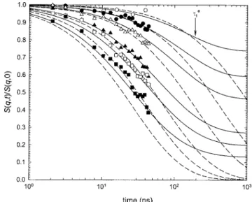
In Fig. 4, the neutron spin-echo results of the PVE sample are compared to the curves calculated from Eq.共7兲at different q values 共ranging from q=0.69 to 1.79 nm−1
or from qa = 3.13 to 8.11 using the rheological value a = 4.53 nm in the calculations兲.2,33
In the calculation for a continuous model, the combination of Ne= 100 and
b = 0.453 nm may be arbitrarily chosen as long as a = 4.53 nm is maintained. With the same Zd value
共0.2214 nm4/ns兲, simultaneous close agreements between
experimental results and theoretical curves at different q val-ues appear to be obtainable. Also shown in Fig. 4 is the comparison with the curves calculated from Eq. 共D3兲 as made by Richter et al. with Zd= 0.28 nm4/ns:36 While
ex-perimental results are in close agreement with the calculated curves at the small q values 共0.69, 0.89, and 1.06 nm−1兲,
significant differences at the large q values共1.38, 1.55, and 1.79 nm−1兲 can be clearly observed. Thus, in the approach of Richter et al., different共apparent兲 Zd values have to be used
FIG. 3. Normalized DSF curves equivalent to those shown in Fig. 2 at
q = 0.5, 1, and 2共or qa=2.5, 5, and 10兲 expressed as a function of the
reduced Rouse variable q2共Z
dt兲0.5 关solid lines calculated from Eq. 共7兲;
dashed lines from Eq.共5兲兴. Also shown is the limiting curve calculated from Eq. 共D3兲共dotted line兲. The double-headed arrows mark the positions of
q2共Z
d1
e
兲1/2= q2共Z
d1兲1/2= q2a2/, while the upward arrow indicates the
position of q2共Z
dq兲1/2= 6.
FIG. 4. Comparison of the measured normalized DSF results共䊊, 쎲, 䉭, 䉱, 䊐, and 䊏 at q=0.69, 0.89, 1.06, 1.38, 1.55, and 1.79 nm−1, respectively兲 of
the PVE sample with the curves 共—兲 calculated from Eq. 共7兲 共with Zd
= 0.2214 nm4ns−1and the combination of N
e= 100 and b = 0.453 nm, giving
a = 4.53 nm兲; with the curves 共---兲 calculated from Eq.共D3兲共as done by
Richter et al.36with Zd= 0.28 nm4ns−1兲. The arrow marks the position of1
e.
to achieve agreements with Eq.共D3兲at different q values as opposed to the same Zd being used in obtaining the shown
simultaneous agreements with Eq. 共7兲. To further illustrate the subtleness regarding the discussed deviations from Eq. 共D3兲, we show both the experimental results and the curves calculated from Eq.共7兲 as a function of the reduced Rouse variable q2共Z
dt兲1/2 in Fig. 5. In the 3⬃4⬎q2共Zdt兲0.5
⬎0.2 region, the experimental data points, though somewhat noisy, can be observed to shift to the faster side at smaller qa as the calculated curves do. To account for statistical noise, we carried out a more careful analysis of the experimental results as described in the following:
In analyzing any set of DSF results here, clearly two factors need to be considered:共1兲 The effect of entanglement if the molecular weight is greater than Meand共2兲 the failure
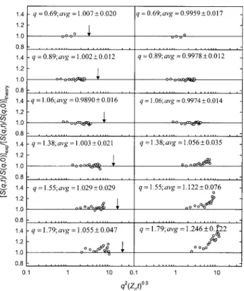
of a Rouse-segment-based theory 关either Eq. 共2兲 or 共7兲兴 at sufficiently large q values as shown in Fig.1. The deviation of Eq. 共7兲 from Eq. 共D3兲 is an issue of entanglement. The agreements between the data points and the theoretical curves can be expressed in terms of the ratios of the experi-mental values to the calculated values; a perfect correlation is indicated by the ratio of 1. The correlations between the data points and Eq. 共7兲 共with Zd= 0.2214 nm4/ns as
deter-mined presently兲 at different q values are compared to those based on Eq. 共D3兲共with Zd= 0.28 nm4/ns as determined by
Richter et al.兲 in Fig.6. In general, for the comparison with Eq. 共7兲, one would show the ratio distribution by adjusting the Zd value such that the average of the ratio values at
different q values is 1. However, at q = 1.55 and 1.79 nm−1,
Eq. 共7兲 may be at the borderline of failure of a Rouse-segment-based theory that becomes serious at larger q 共Fig.1兲. Thus, the ratio distribution shown in Fig.6 is pre-sented in such a way that the average of the ratio values at the four smaller q values is 1—the Zd value as used in the
comparison of experiment and theory shown in Figs.4and5 has been determined this way. This allows room for devia-tions from Eq. 共7兲 at q = 1.55 and 1.79 nm−1 to show up if
noticeable failure of the Rouse-segment-based theory exists. As opposed to the large deviations at q = 1.38, 1.55, and 1.79 nm−1 in the case of comparing with Eq. 共D3兲 共right
panel of Fig. 6兲, one observes close correlations in the case of comparing with Eq.共7兲with only small noticeable devia-tions at q = 1.55 and 1.79 nm−1 共left panel of Fig.6兲. These
small deviations are of magnitude similar to those that can be observed in a similar comparison—under the same condition that the average of the ratio values at the four smaller q values is 1—between the data of the PIB sample and Eq. 共2兲at similar q values 共1.5–2 nm−1兲 and over the same ranges of q2共Zdt兲0.5 as shown in Fig. 7. Furthermore, the
value Zd= 0.2214 nm4/ns obtained from matching the DSF
curves with Eq. 共7兲 is in close agreement with the values 关Zd= 0.238共⫾20%兲 共Ref. 37兲兴 obtained from analyzing the
incoherent neutron scattering results of the protonated sample in terms of Eq. 共9兲. The existence of deviation from the limiting form is also indicated by the Zd value
共0.28 nm4/ns兲 obtained by Richter et al. at the three lowest q
values 共Fig. 4兲 being significantly larger than these two mutually consistent values.
The above analyses support that Eq.共7兲is as valid for an FIG. 5. Comparison of the measured normalized DSF results共the same as in
Fig.4兲 of the PVE sample with the curves 共—兲 calculated from Eq.共7兲共the
same as in Fig. 4兲, both expressed as a function of the reduced Rouse
variable, q2共Z
dt兲1/2. The arrows from the top to the bottom mark the
posi-tions of q2共Z
d1
e兲1/2= q2a2/ at q = 0.69, 0.89, 1.06, 1.38, 1.55, and
1.79 nm−1, respectively.
FIG. 6. The ratios of the normalized DSF data of the PVE sample to the values calculated from Eq.共7兲共the left panel; the same as in Fig.5兲 vs the
ratios of the same data to the values calculated from Eq.共D3兲共the right panel; the same as in Fig. 4兲. The arrows 共in the left panel兲 mark the
positions of q2共Z
d1
e
兲1/2= q2a2/.
entangled system as Eq.共2兲is for an entanglement-free sys-tem as far as the t⬍1e region is concerned. In other words, the comparison of the data of the PVE sample with Eq. 共7兲 supports the existence of deviation from the limiting form in the range 5⬎qa⬎1 as discussed in Sec. IV. This conclusion does not support the observation of the crossover from ␣ relaxation to Rouse dynamics claimed by Richter et al.36on the basis of the q dependence of the Zdvalues obtained from
their analyses in terms of Eq.共D3兲.
We have used the rheological value of a in Eq. 共7兲 to calculate the curves for the PVE sample shown in Figs.4–7. As the tⰆ1eto t⬍1eregion is not very sensitive to a small change in a, using a value larger by 20% as shown possible by monitoring the q-split plateaus below does not lead to a different conclusion.
B. q-split plateaus
The dependence on the entanglement length a is not as strong in the time region t⬍1eas in the t⬎1eregion, where the q-split plateaus occur. By monitoring the agreement be-tween experiment and theory regarding the q-split plateaus, one may adjust the a value to be substituted into Eq.共7兲. In Fig.8, the neutron spin-echo results of the PEB-2 sample at 509 K are compared to the curves calculated from Eq. 共7兲 using a = 4.0 nm, which is about 16% greater than the rheo-logical value of 3.44 nm obtained at 413 K.2,33The compari-son is made with Zd= 7 nm4/ns, which is quantitatively
con-sistent with the incoherent scattering results.38 Under this condition, there are four features in the shown comparison
between theory and experiment:共1兲 In the short-time region, the data points at different q values “group” together in the same region as the curves calculated from Eq. 共7兲. Because there are too few data in the short-time region, the deviations of Eq.共7兲from Eq.共D3兲in the region cannot be assessed in this case as in the case of the PVE sample. However, within the noises of the data points, the experimental results are not in disaccord with the analyses of the results of the PVE sample given above. 共2兲 The positions in time of the steep declines as clearly identifiable at the q values: 0.96 and 1.15 nm−1are in close agreement with the theoretical
predic-tions.共3兲 The heights of the plateaus and their distribution in the long-time region t⬎1e as a function of q are well pre-dicted by the theory. The plateau height level depends on the unitless quantity qa only. The large separation between the two plateaus at the two largest q values共0.96 and 1.15 nm−1兲 corresponds to a change that can be caused by an ⬃20% difference in the a value if q is kept the same. Thus, the close matching of the q-split plateau distribution between experi-ment and Eq. 共7兲 represents a high-resolution determination of the a value.共4兲 At different q values, the general positions of turning from a steep decline to a plateau are in agreement with the predictions of Eq. 共7兲, despite the noise associated with the data points. The turns are sharper in the theoretical curves than in the experiment results. In a consistent and systematic way at different q values, the experimental values deviate from the calculated curves to the higher side around FIG. 7. Comparison of the ratios of the normalized DSF data of the PVE
sample to the values calculated from Eq.共7兲共the left panel; the same as in Fig.6兲 and the ratios of the data of the PIB sample to the values calculated
from Eq.共2兲共the right panel兲 at similar q values and over similar ranges of
q2共Z
dt兲1/2. The arrows mark the positions of q2共Zd1
e兲1/2= q2a2/共in the left
panel兲 and q2共Z
d1兲1/2= q2R2/共in the right panel兲.
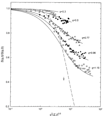
FIG. 8. Comparison of the normalized DSF results共䊊, 쎲, 䉭, 䉱, and 䊐 at
q = 0.3, 0.5, 0.77, 0.96, and 1.15 nm−1, respectively兲 of the PEB-2 sample
with the curves calculated from Eq.共7兲共with the combination of Ne= 100
and b = 0.4 nm, giving a = 4 nm兲, both expressed as a function of the reduced Rouse variable, q2共Z
dt兲1/2. The comparison is made with Zd= 7 nm4ns−1.
The upward arrows from the top to the bottom mark the positions of
q2共Z
d1
e
兲1/2= q2a2/at q = 0.3, 0.5, 0.77, 0.96, and 1.15 nm−1, respectively.
The limiting curve for qa→⬁ 关Eq.共D3兲兴 is shown as the dashed line; the downward arrow indicates the position of q2共Z
dq兲1/2= 6.
the bending point; the data points converge with the calcu-lated plateaus at long times. The above listed features indi-cate that the Rouse–Mooney model as presented in this paper has captured the basic elements of the mechanism for the relaxation of the DSF curves and their converging to a pla-teau. The systematic deviations are most likely due to less-than-perfect validity of the model. As shown in Fig. 8, the bending points occur at times longer but not much longer than t =1e, and higher experimental values start to appear at the timescales of 1e. These deviations from the theoretical curves suggest that any improvement on the model should affect the slowest mode of the Rouse–Mooney process most, lengthening its effective relaxation time.
From the line-shape analyses of viscoelastic responses G共t兲 and G*共兲 in terms of the ERT,2,7–12it is known that the
chain-slippage共through entanglement links兲 processX共t兲 is
responsible for the decline in modulus right after the end of the Rouse–Mooney process A共t兲. Due to the relaxation of X共t兲, the modulus drops fromRT/Me关modulus at the end
of A共t兲兴 to 4RT/5Mein G共t兲. The relaxation time of the X共t兲 process, X, decreases linearly with decreasing
molecular weight. The X for the PEB-2 sample with Mw
= 1.9⫻105 is estimated to be about 100 times larger than
1 e
;39 any effect that can come fromX共t兲 should be far
be-yond the time windows of the DSF measurements. In other words, the PEB-2 sample with Mw= 1.9⫻105 may be
con-sidered as a well-entangled system suitable for comparing its neutron spin-echo results with Eq. 共7兲. As observed in the study of a series of PEB-2 samples,40 when the molecular weight is low enough, the heights of the plateaus at different q values drop more and the slopes on the plateaus are en-hanced with decreasing molecular weight. These symptoms suggest an effect involving theX共t兲 process, which relaxes
the fixed-end assumption more with decreasing molecular weight. In particular, at Mw= 1.24⫻104 共the smallest
mo-lecular weight studied in Ref.40兲, theXvalue is only about
six times1e; the effect of X共t兲 is well within the time
win-dows of the DSF measurements. Thus, as expected, consid-erable drops in the heights of the plateaus are observed in the case of the sample with Mw= 1.24⫻104.
VI. DISCUSSION
A. The q-split plateaus and the boundary conditions
As opposed to Eq.共7兲 being for strands with both ends fixed, Eq.共5兲is for chains free at both ends, yet trapped in a domain with a diameter of
冑
N0b. Here we compare Eqs.共5兲and共7兲under the situation that the domain diameter for the former is the same as the entanglement length for the latter, namely, a =
冑
Neb =冑
N0b. As shown in Appendix D, both Eqs.共5兲and共7兲converge to the same limiting form关Eq.共D3兲兴 in the time region of tⰆ1or 1
e共 1and1
e
are the same as N0
and Ne are treated as equivalent here兲 for qaⰇ1 共or qa
⬎10兲. However, in the region ⬃7⬎qa⬎ ⬃1, Eq.共5兲gives a very different distribution of q-split plateaus from Eq. 共7兲 共Figs.2and3兲. The comparison of Eqs.共D1兲and共D2兲 indi-cates that in the short-time region, Eqs.共5兲and共7兲converge to the limiting form关Eq.共D3兲兴 from the opposite sides 共see Fig.3兲. As opposed to Eq.共7兲being successful, as shown in
Sec. V, Eq.共5兲is far from being able to describe the experi-mental results. The drastic differences between Eqs.共5兲 and 共7兲 indicate that the fixed-end boundary conditions are an essential ingredient—confinement alone is not sufficient— for the observed distribution of the q-split plateaus. This con-clusion logically leads to the mechanism of chain slippage through entanglement links as pictured in the Doi–Edwards model—as a chain conformation, say, deformed, has to relax completely eventually without involving a chain break-and-link process. Extensive studies1,2,7–12,41–44 of polymer viscoelastic responses—including the successful prediction of the damping factor in the studies of nonlinear viscoelasticity1,2,41–44—have supported the slip-link picture as embodied in the Doi–Edwards model.1,2,26The analyses of the spin-echo results as presented in this paper further support the model on the microscopic level.
B. Comparisons with existing models
Models have been developed for understanding the co-herent dynamic scatterings of single entangled chains by de Gennes,45Ronca,46and des Cloizeaux.47These theories have been used to explain the q-split plateaus with different de-grees of success; performances of these theories have been compared.6,24,48 As de Gennes’ theory has often been used for data analyses in the literature and appears to give the entanglement length closest to the rheological value among the three theories, we shall mainly focus on its comparison with Eq.共7兲.
de Gennes’ theory and Eq. 共7兲 are based on different starting points: As opposed to the fixed-end boundary condi-tions for each entanglement strand in the latter case, de Gennes’ theory imposes a tensile force 3kT/a 共as given by the Doi–Edwards theory1,2,26 for maintaining the primitive-chain contour length L = R2/a兲 on both ends of the chain. de Gennes’ theory considers fluctuations of the segmental den-sity along the primitive chain, which has the average value given by N0/L=Ne/a=Ne
0.5/b, and terms it as “local
repta-tion.” The sort of process considered by deGennes is physi-cally similar to those responsible for the X共t兲 and B共t兲
processes in the ERT.2,7–12The local reptation is regarded in de Gennes’ theory as responsible for the main dynamics ob-served in the coherent scattering from one reptating chain, if the chain is extremely well entangled. Both the present pro-posed Rouse–Mooney model and de Gennes’ picture expect that, given enough time, reptation will eventually be fully carried out randomizing the whole primitive chain or tube. The main difference between the two is that the former fo-cuses on the dynamics within one step length of the primitive chain as opposed to the latter being intended for dynamics beyond one step length. In de Gennes’ picture, the slip-link “structure” and the existence of the Rouse–Mooney process 共including chain motions perpendicular to the primitive path兲 before chain slippage has the chance to take place are ignored. In accord with this picture, the condition q2a2Ⰶ1
Ⰶq2R2 has been used at several approximation steps in the
derivation of de Gennes’ theoretical result.
After making additional approximations, de Gennes obtained a DSF function consisting of two separate terms: This article is copyrighted as indicated in the article. Reuse of AIP content is subject to the terms at: http://scitation.aip.org/termsconditions. Downloaded to IP:
A time-dependent term characterized by the time constant
q= 36/Zdq4—independent of the length scale a—is to
ac-count for the relaxation in the short-time region. The other term 共the so-called creep term兲, which can justifiably be re-garded as time independent for a well-entangled sample, is responsible for the existence of plateaus at long times.
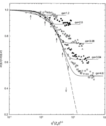
The comparisons of the experimental results of the PEB-2 sample with de Gennes’ equation as well as with Eq.共D3兲are shown in Fig.9.49The comparisons at different q values are made using the same values of Zd
共=7 nm4/ns兲24,35
and a 共=4.9 nm兲 as obtained by Wischnewski and Richter 共Fig. 1 of Ref. 24兲 for giving an “optimum” fit. Note this Zd value and that used in the
com-parison with Eq.共7兲 shown in Fig.8 are equal, both being consistent with the incoherent scattering results.38 With a = 4.9 nm, the results shown in Fig.9 cover the range from qa = 1.47 to 5.64 as opposed to the condition q2a2Ⰶ1
Ⰶq2R2 required in the development of de Gennes’ theory.
This represents a fundamental inconsistency that would un-dermine the soundness of the analysis in terms of de Gennes’ theory.
The characteristic time in de Gennes’ equation is located at the fixed position q2共Zdq兲1/2= 6 in Fig.9as opposed to the
position of the relaxation time of the lowest Rouse–Mooney mode, as given by q2共Zd1
e兲1/2= q2a2/, moving to the right
side with increasing q in Fig.8. These positions are indicated by arrows in Figs. 8 and 9. To a large degree due to this difference, while the curves calculated from Eq. 共7兲 move closer to Eq. 共D3兲 with increasing q over the range 1⬃4
⬎q2共Z
dt兲0.5⬎0.1, the curves calculated from de Gennes’
equation deviate more from it. This contrast represents a gap between the short-time and long-time regions in de Gennes’ theory. Thus, Richter et al.24,35,38,48have resorted to Eq.共D3兲 to determine the Zd value needed in comparing the
experi-mental results with de Gennes’ equation emphasizing com-parisons over the long-time region where the q-split plateaus occur. The difference between using Eq. 共D3兲 and using Eq. 共7兲 to determine the Zd value and its consequence for
drawing conclusion have been analyzed and discussed in de-tail in Sec. V A for the PVE sample. The discussed gap is very much responsible for the large deviations of the experi-mental results on the high side from de Gennes’ equation over the short-time region at q = 0.96 and 1.15 nm−1 and on the low side at q = 0.3 and 0.5 nm−1 as can be clearly ob-served in Fig.9. Including the plateau regions, unlike in the comparison between experiment and Eq. 共7兲, the observed deviations from de Gennes’equation do not appear to be sys-tematic at different q values. This may be unavoidable due to the inconsistency between the range of qa as emerging from the analysis-obtained results and that covered by de Gennes’ theory.
The natural reduction of Eq.共7兲to Eq.共D3兲allows us to display a full range of DSF curves as a function of the re-duced Rouse variable q2共Z
dt兲1/2in a unified way as shown in
Fig. 3. This is a property not shared by the other theories. The shown full range forms a framework or “map,” with respect to which different regions of the DSF curves at dif-ferent q values can be located and studied in a consistent manner. One may notice that the Langevin equation and nor-mal modes involved in deriving Eq. 共7兲 are the same as in deriving theA共t兲 relaxation process2,10 as part of the ERT.
Thus, data analyses in terms of Eq. 共7兲 can benefit directly from the past studies of polymer viscoelasticity in terms of the ERT.2,7–12
The entanglement length a calculated from the plateau modulus GN has been regarded as a characteristic quantity
related to entanglement. It has been well established that the number of entanglement strands per cubed entanglement length nt is a universal constant.2,33,50,51 In addition to the
theoretical distinctions of Eq. 共7兲 pointed out above, the a value obtained from analyzing the DSF results of the PEB-2 sample in terms of Eq.共7兲 is closer to the rheological value than in terms of the other theories. For PEB-2 at 509 K, the a values obtained from the various analyses24,48 are 4 nm 关Eq. 共7兲兴, 4.6–4.9 nm 共de Gennes兲, 4.74 nm 共Ronca兲, and 5.98 nm 共des Cloiseaux兲 versus the rheological value of 3.44 nm at 413 K.2,33,51 Exempt from effects of the slower ERT modes of motionX共t兲,B共t兲, andC共t兲, a likely reason
for the a value of a well-entangled system obtained from analyses in terms of Eq. 共7兲 to be slightly higher than the rheological value is the temperature difference. For instance, in the case of PEB-17.6关poly共ethylene-co-bulene兲 with 17.6 ethyl branches per 100 carbons兴,2,33,51
calculations from the plateau modulus values give a = 4.71 nm at 413 K and a = 3.75 nm at 298 K. This example suggests that an⬃100 K difference in temperature can cause a difference in the a value as large as 25%. Such an effect may be responsible for the difference between 4 nm at 509 K as obtained from ana-FIG. 9. Comparison of the normalized DSF results共䊊, 쎲, 䉭, 䉱, and 䊐 at
q = 0.3, 0.5, 0.77, 0.96, and 1.15 nm−1, respectively兲 of the PEB-2 sample
with the curves calculated from de Gennes’ equation共with a=4.9 nm兲, both expressed as a function of the reduced Rouse variable, q2共Z
dt兲1/2. The
comparison is made with Zd= 7 nm4ns−1. The limiting curve for qa→⬁
关Eq.共D3兲兴 is shown as the dashed line. The arrow marks the position of
q2共Z
dq兲1/2= 6.
lyzing the DSF curves in terms of Eq.共7兲and the rheological value of 3.44 nm at 413 K for the PEB-2 polymer.
VII. SUMMARY
The theoretical DSF function forms based on the Rouse and Rouse–Mooney models, both discrete and continuous, are given and their calculated results are compared in this paper. It has been shown that it is sufficient to use the con-tinuous Rouse–Mooney model to analyze the coherent neu-tron scatterings from single well-entangled chains in the q region where a Rouse-segment-based theory is applicable. In the analyses, a =
冑
Neb and Zd= 3kTb2/are the onlyadjust-able parameters, wherein for all practical purposes, an arbi-trary pair of sufficiently large Neand small b may be chosen
共Appendix B兲.
Two characteristics are identified in the DSF functional form for well-entangled single chains 关Eq. 共7兲兴: One is the deviations from the limiting form 关Eq. 共D3兲兴 in the region ⬃4⬎q2共Z
dt兲0.5⬎ ⬃0.1 共corresponding to a time region from
tⰆ1e to t⬍1e兲 to the faster side as qa is in the range 1–5. The other is the q-split plateaus that can be experimentally observed in the time region t⬎1e when qa is between ⬃1 and ⬃7, allowing a high-resolution determination of the a value. The validity of these two characteristics is well sup-ported by the comparisons between theory and experiment at different q values in the respective regions. The entangle-ment length a extracted from analyzing the DSF line shapes of the studied well-entangled PEB-2 polymer is in agreement with the rheological value within 20%. It is shown that the small difference may be due to the large difference between the temperatures at which the two values are respectively determined.
From this study, it is shown that the fixed-end boundary conditions assumed for the dynamic behavior of a well-entangled entanglement strand are essential for obtaining the distribution of the q-split plateaus as observed experimen-tally by the neutron spin-echo spectroscopy. This strongly supports that the Rouse–Mooney model is applicable micro-scopically as it has been shown to be so macromicro-scopically in the studies of viscoelastic-response functions.2,7–12 This also represents a support on the microscopic level for the mecha-nism of chain slippage through entanglement links as em-bodied in the Doi–Edwards theory.
Equation共7兲reduces to the limiting form Eq.共D3兲 natu-rally allowing a full range of DSF curves to be presented in terms of the reduced Rouse variable q2共Z
dt兲1/2 in a unified
way. The displayed full range represents a framework or map, with respect to which different regions of DSF may be located and studied in a consistent manner.
ACKNOWLEDGMENTS
This work is supported by the National Science Council 共NSC 96-2113-M-009-020-MY3兲. We thank Professor Rich-ter and Professor Colmenero for providing us with the neu-tron spin-echo data of the PEB-2, PIB, and PVE samples.
APPENDIX A: THE DISCRETE ROUSE AND ROUSE–MOONEY MODELS
The DSF based on the discrete Rouse model is given by52 S共q,t兲 = 1 N0 exp共− q2DGt兲 ⫻
兺
n=1 N0兺
m=1 N0 exp冋
−q 2 6b 2兩m − n兩 −2q 2b2 3N0兺
p=1 N0−1 f共m,p,N0兲f共n,p,N0兲 ⫻冋
1 − exp冉
− t p冊
册
册
, 共A1兲 where DG= kT N0 , 共A2兲 f共m,p,N0兲 =兺
s=1 N0−1 s N0 sin冉
sp N0冊
−兺
s=m N0−1 sin冉
sp N0冊
, 共A3兲 and p= K 2M2 12N02sin2共p/2N0兲 , p = 1,2,3, . . . ,N0− 1. 共A4兲The DSF of the discrete Rouse–Mooney model is given by52 S共q,t兲 = 1 Ne ⫻
兺
n=1 Ne兺
m=1 Ne exp冋
−q 2 6 b 2兩m − n兩 −q 2b2 6Ne兺
p=1 Ne−1 h共m,p,Ne兲h共n,p,Ne兲 ⫻冋
1 − exp冉
− t p e冊
册
册
, 共A5兲 with h共m,p,Ne兲 = sin冉
mp Ne冊
sin冉
p 2Ne冊
共A6兲 and p e = K 2M e 2 12Ne2sin2共p/2Ne兲 , p = 1,2,3, . . . ,Ne− 1. 共A7兲As expected, when N0→⬁ or Ne→⬁, Eqs. 共A1兲 and
共A5兲 reduce to Eqs.共2兲and共7兲, respectively, and Eqs.共A4兲 and共A7兲to Eqs.共3兲and共8兲, respectively.
APPENDIX B: DYNAMIC PARAMETERS IN ROUSE-SEGMENT-BASED THEORIES
In a Rouse-segment-based theory 共the Rouse theory or the ERT兲, the relaxation times can be expressed as a product of the frictional factor K and a structural factor,2,7–12which is a function of molecular weight M and/or entanglement This article is copyrighted as indicated in the article. Reuse of AIP content is subject to the terms at: http://scitation.aip.org/termsconditions. Downloaded to IP:
lecular weight Me. From analyzing the viscoelastic results in
terms of a Rouse-segment-based theory, K is the key dy-namic parameter that can be extracted. For instance, in the case of using the ERT to analyze the viscoelastic responses: G共t兲 and J共t兲 of entangled nearly monodisperse polystyrene melts, the obtained K values关for theX共t/X兲,B共t/B兲, and C共t/C兲 processes兴 are independent of molecular weight as
expected from the theory共see Table 1 of Ref.7兲.2,7–11From analyzing the G共t兲 and G*共兲 line shapes of entangled
poly-styrene binary-blend solutions in terms of the linear combi-nation of the ERT and the Rouse theory, the values of K as embodied in the two theories have been found to agree within 20%.2,9,12 Very importantly, this agreement indicates that the Rouse theory and the ERT have the same footing at the Rouse-segmental level.关Note that the frictional factor for the Rouse–Mooney process A共t/A兲, denoted by K
⬘
, islarger than K by a factor RK共M /Me兲 that depends on the
normalized molecular weight M/Me. As detailed in Refs.2,
9, 11, and 12, RK共M /Me兲 being greater than 1—declining
from the plateau value of 3.3 at M/Me⬎10 to the limiting
value 1 as M/Me→1—represents dynamic anisotropy due to
topological constraint of entanglements. The following discussion on K is also applicable to K
⬘
.兴Here, we would like to show that the frictional factor K is equivalent to the parameter Zd that has often been
extracted from the coherent dynamic neutron scattering studies. The entanglement distance a can be expressed as
a2= K⬁Me, 共B1兲
where K⬁ is defined as the ratio of the mean square end-to-end distance of a polymer to its molecular weight,
K⬁= R2/M, which can be determined by static neutron
scattering.1,2,33,50,51 One may also write a2= Neb2=
Me
mb
2. 共B2兲
The combination of Eqs.共B1兲and共B2兲leads to
b2= K⬁m. 共B3兲
Since K⬁is a constant, b2is linearly proportional to m. Using this relation, Eq. 共4兲is obtained.
As being inversely proportional to K关Eq. 共4兲兴, Zd may
replace K playing the role of the key dynamic parameter. Even though in the neutron spin-echo studies of polymers, the continuous Rouse model is always used as in this study, Zdtheoretically remains the relevant key dynamic parameter
because of the scaling relations ⬀m and b2⬀m. For
example, Eq.共D3兲is a universal function of q2共Z dt兲1/2.
APPENDIX C: THE BASIC DSF FORM OF A
WELL-ENTANGLED CHAIN UNDER THE CONDITION
qRš 1
In a well-entangled labeled chain, as the entanglement points共slip links兲 are regarded as fixed, the modes of motion of an entanglement strand are isolated from those of others, and segments belonging to different entanglement strands are not correlated. Denoting entanglement strands by k and l, and beads by n and m, the DSF of the labeled chain can be reduced as follows: S共q,t兲 = 1 N0
兺
k=1 N兺
l=1 N兺
n=1 Ne兺
m=1 Ne 具exp关iq · 共Rn k共t兲 − R m l共0兲兲兴典 = 1 N0兺
k=1 N兺
n=1 Ne兺
m=1 Ne 具exp关iq · 共Rn k共t兲 − R m k共0兲兲兴典 + 1 N0兺
k=1 N兺
l⫽k N冓
兺
n=1 Ne exp共iq · Rn k共t兲兲冔冓
兺
m=1 Ne exp共− iq · Rm l共0兲兲冔
= N N0n=1兺
Ne兺
m=1 Ne 具exp关iq · 共Rn共t兲 − Rm共0兲兲兴典 + 1 N0冓
兺
k=1 N兺
n=1 Ne exp共iq · Rn k共t兲兲冔冓
兺
l=1 N兺
m=1 Ne exp共− iq · Rm l共0兲兲冔
− 1 N0兺
k=1 N冓
兺
n=1 Ne exp共iq · Rn k共t兲兲冔冓
兺
m=1 Ne exp共− iq · Rm k共0兲兲冔
. 共C1兲Because at any moment, the beads 兵Rn共t兲其 are distributed
randomly over RⰇq−1, the second and third terms of
Eq. 共C1兲 are negligible, and Eq. 共C1兲 reduces to the form given by Eq.共6兲.
APPENDIX D: LIMITING DSF FORM IN THE SHORT-TIME REGION WHEN q2N
0b2 OR q2Neb2š 1 When q2N0b2or q2Neb2Ⰷ1, we may limit consideration
to the time region tⰆ1in Eq.共5兲关equivalently in Eq.共2兲, as
DGis very small and exp共−q2DGt兲 is practically equal to 1 in
the short-time region兴 or tⰆ1 e
in Eq.共7兲, respectively. In the
short-time domain, the respective summations over p in the exponents of these equations are dominated by large p. Under p being large, the underlined terms in the factors
2 cos