使用者輔助的模型化簡

國

立

交

通

大

學

資訊工程系

碩 士 論 文

使用者輔助的模型化簡

User-Assisted Mesh Simplification

研究生：彭其瀚

指導教授：莊榮宏 博士

User-Assisted Mesh Simplification

Student: Chi-Han Peng

Advisor: Dr. Jung-Hong Chuang

Department of Computer Science and Information Engineering

National Chiao Tung University

ABSTRACT

Many simplification methods have been proposed to generate multiresolution models for real-time rendering applications. Practitioners have found that these methods fail to produce satisfactory result when models of very low polygon count are desired. This is due to the fact that the existing methods take no semantic or functional metric into ac-count, and moreover, each simplification metric has its own strength and weakness as well in preserving geometric features. To overcome such limitations, we propose an interactive system that allows users to refine unsatisfactory regions on any level of simplification. Our approach consists of two stages. The first stage involves modifying the simplification order to postpone the collapsing for edges in the unsatisfactory regions. The second stage is a local refinement tool aiming to provide fine tuning on the simplified meshes. The ma-jor advantage of our approach is that our system provides a predictable and quantifiable control over the refining process. The system is packed as a 3ds Max plugin, so users can easily integrate our system into the digital content creation process.

Keywords: level of detail, mesh simplification, user-assisted simplification.

Acknowledgments

I would like to thank my advisors, Dr. Jung-Hong Chuang, for his inspirations, guid-ance and patience for the past years.

I also appreciate all my classmates and members of the CGGM laboratory, for their assistances and discussions. Especially, thank Tan-Chi Ho for guidance for this thesis and Chih-Chun Chen for his LOD system framework used in the implementation of this thesis.

I am grateful to my mother, father and my brother for their support, encouragement and love.

Contents

2.3.1 Quadric Error Metrics (QEM) . . . 6

2.3.2 Appearance-Preserving Simplification . . . 7

2.4 View-Dependent LOD . . . 9

2.4.1 View-Dependent Refinement of Progressive Meshes . . . 9

2.4.2 Truly Selective Refinement of Progressive Meshes . . . 11

2.5 User-Assisted Mesh Simplification . . . 13

2.5.1 Zeta: a Resolution Modeling System . . . 14

2.5.2 Semisimp . . . 14

2.5.3 User-Guided Simplification . . . 16

3.2 Weighting Simplification Cost . . . 22

3.3 Local Refinement . . . 26

4 Experimental Results 31 4.1 Weighting Tests . . . 32

4.2 Local Refinement Tests . . . 39

4.3 Comparisons of Weighting and Local Refinements . . . 42

4.4 Case Studies . . . 47

4.4.1 Case1: Armadillo . . . 47

4.4.2 Case2: Liberty . . . 49

4.4.3 Case3: Parasaur . . . 51

5 Conclusion and Future Work 53 5.1 Summary . . . 53

5.2 Future work . . . 53

Bibliography 55

List of Figures

2.1 The concept of LOD [17]. . . 4

2.2 Edge collapse and vertex split [9]. . . 5

2.3 PM sequence [14]. . . 5

2.4 APS Texture deviation [15]. . . 8

2.5 Sampling the texture deviation [12]. . . 8

2.6 Approximates global texture deviation using bounding box. [12]. . . 9

2.7 View-dependent PM [10]. . . 10

2.8 Vertex hierarchy [10]. . . 10

2.9 Neighboring configurations of edge collapse and vertex split [10]. . . 11

2.10 Vertex splits dependency problem [13]. . . 11

2.11 Dual pieces [13]. . . 12

2.12 PM sequence and the corresponding dual pieces [13]. . . 13

2.13 Zeta’s vertex decimation operator [1]. . . 14

2.14 Selective refinement in Zeta [1]. . . 15

2.15 Geometric manipulation in Semisimp [7]. . . 15

2.16 Hierarchy manipulation in Semisimp [7]. . . 16

2.17 The effects of adaptive weighting of quadrics [22]. . . 16

2.18 An example of contour constraints [22]. . . 17

3.1 System overview. . . 21

3.2 Notations of the weighting scheme. . . 22

3.3 Illustration of the first step in the weighting scheme. . . 24

3.4 Illustration of the second step in the weighting scheme. . . 25

3.5 An example of weighting. . . 25

3.6 The concept of our cost adjustment scheme. . . 27

4.1 The testing models. . . 31 4.2 The quality improvement on weighted regions of Armadillo’s simplification. 32 4.3 The sacrifice of quality on unweighted regions of Armadillo’s simplification. 33 4.4 The quality improvement on weighted regions of Liberty’s simplification. . 34 4.5 The sacrifice of quality on unweighted regions of Liberty’s simplification. . 36 4.6 Effects of multiple weighting. . . 37 4.7 The effect of weighting on simplifications with default and non-default ratios. 38 4.8 The effects of cost adjusting for the cost distribution over the entire mesh. 39 4.9 Using local refinement to gradually refine Armadillo’s left eye. . . 40 4.10 Edge collapses executed by local refinements with and without cost

adjust-ments. . . 41 4.11 Comparing the refined simplifications by weighing, local refinements and

both. . . 44 4.12 Recover sharp features on the Armadillo’s simplification with 500 faces by

weighting. . . 45 4.13 Recover sharp features on the Armadillo’s simplification with 500 faces by

local refinements. . . 45 4.14 Recover sharp features on the Armadillo’s simplification with 1000 faces by

weighting. . . 46 4.15 Recover sharp features on the Armadillo’s simplification with 1000 faces by

local refinements. . . 46 4.16 Comparison of the unrefined and the refined simplifications with 1000 faces

of Armadillo. . . 48 4.17 Closer comparisons between the unrefined (left) and refined (right)

simpli-fications with 1000 faces of Armadillo. . . 48 4.18 Comparison of the unrefined and the refined simplifications with 1000 faces

of Liberty. . . 50 4.19 Comparison of the unrefined and the refined simplifications with 760 faces

of Parasaur. . . 51

List of Tables

4.1 Comparing geometric errors of Armadillo’s weighted simplification with 2000 faces . . . 33 4.2 Comparing geometric errors of Liberty’s weighted simplification with 1000

faces . . . 34 4.3 The effect of weighting on simplifications with default and non-default ratios 35 4.4 Geometric errors of performing local refinements on the left eye of the

Armadillo model . . . 40 4.5 Geometric errors on Armadillo’s refined simplifications by weighting, local

refinements and both . . . 42 4.6 Comparing geometric errors of Armadillo’s unrefined and refined

simplifi-cations . . . 47 4.7 Comparing geometric errors of Liberty’s unrefined and refined simplifications 49

C H A P T E R

1

Introduction

1.1

Motivation

Polygonal meshes has become the most common model presentation in 3D computer graphic applications. With the development of 3D scanning technologies and modeling tools, raw meshes can be composed of thousands to millions of polygons. To process such large models efficiently, many mesh simplification algorithms have been proposed to decrease the complexity of models while maintaining similarity with the original model.

Several algorithms have been proposed to derive the so called progressive meshes by using a series of primitive collapsing, such as edge collapsing, in the increasing order of simplification cost. These algorithms usually differ in how the simplification cost is measured. Among others, we list quadric error metric (QEM) [6], appearance preserving simplification (APS) [12] and image driven simplification (IDS) [16]. QEM measures the geometric error between the simplified mesh and original mesh, APS represents the texture deviation resulting from the simplification, and IDS calculates the visual difference. Each of these well known metrics has its own strength and weakness in preserving geometric and texture features. Moreover, all of these metrics do not take semantic or functional features into account. As a result, practitioners have found that these metrics alone are not able to produce satisfactory result when the simplified mesh of low-polygon count are expected.

To overcome such limitations, user-assisted simplification has been proposed recently [1] [5] [7] [22]. For example, in user-guided simplification [5] [22], users revise the simplified mesh by re-ordering the simplification order such that edges in the selected region will be

collapsed later. The re-ordering of edge collapses is done by multiplying the simplification cost of these edges with a user-specified multiplier. These methods suffer from several problems. For example, the value of the multiplier has no direct relation to the resulting simplification. In consequence, the multiplier is usually chosen in a trial and error basis. Moreover, the appropriate multiplier may be different for different error metrics since the ranges of the different metrics vary greatly.

1.2

Contributions

We propose a user-guided framework that allows users to improve the quality of simplified meshes by existing error metrics, such as QEM and APS. The framework consists of two stages. The first aims to reorder the edge collapse by a weighting scheme. The proposed weighting scheme differs from the previous ones in that the weighting values are automatically derived based on how many more vertices users expect to have in the interested region. The second is a local refinement scheme aims to fine tune the mesh resulting from the first stage.

Our system is packed as a 3ds Max plugin, which offers an easy-to-use user interface and is compatible with existing applications, and in consequence, can be integrated into the digital content creation process.

1.3

Thesis Organization

In chapter 2 we will introduce background and previous work related to this thesis. Chap-ter 3 presents our user-assisted mesh simplification schemes. In chapChap-ter 4 some implemen-tation details and the experimental results will be given, and chapter 5 is the conclusions and discusses of future work.

C H A P T E R

2

Related Work

In this chapter, a review on related work of our method will be given. Section 2.1 in-troduces the general architecture of level of detail (LOD) modeling. In section 2.2, pro-gressive meshes [9], a widely-used continuous presentation of multi-resolution modeling is described. In section 2.3, we will introduce two methods of measuring error of mesh simplification operations. In section 2.4, we will introduce two methods of view-dependent LOD, including view-dependent refinement of progressive meshes [10] and truly selective refinement of progressive meshes [13]. In the last section, we will describe the methods of user-assisted simplification.

2.1

Level-of-detail Modeling

Level-of-detail (LOD) modeling aims to represent a complex mesh with several levels of detail, and from which an appropriate level is selected at run time to represent the original mesh, as shown in Figure 2.1. A number of methods have been proposed in the literature. Most methods simplify the given mesh by using a sequence of primitive reduction operations, such as edge collapse [11], triangle collapse [8], vertex clustering [19], vertex removal [20], and multi-triangulations [4].

The primitive reduction operation can be organized in various orders. The simplest way is to perform the operations in arbitrary order. A more sophisticate approach is to perform the operations in the increasing order of simplification cost, which is analogous to the greedy algorithm.

Several error metrics have been proposed to determine the cost of primitive reduction

69,451 triangles 2,502 triangles 251 triangles 76 triangles

Managing model complexity by varying the level of detail used for rendering small or distant objects. Polygonal simplification methods can create multiple levels of detail such as these.

Figure 2.1: The concept of LOD [17].

operation, such as quadric error metrics (QEM) [6], appearance-preserving simplification (APS) [12], image-driven simplification (IDS) [16] and perceptually guided simplification of lit, textured meshes [18]. Different error metric has its strength in preserving certain properties of the original mesh. For example, quadric error metrics aims to preserve the geometric accuracy during the simplification process, and image-driven simplification aims to preserve the visual fidelity between the simplified mesh and the original mesh.

LOD can be discrete [3] or continuous [9]. Discrete LOD creates various levels of detail for the original mesh, each of which has no direct relation to others and cannot be derived from other levels. At run-time, an appropriate level of detail is chosen to present the original mesh. On the other hand, continuous LOD creates a data structure encoding a continuous spectrum of detail so that at run-time the desired level of detail can be extracted from this structure. The progressive meshes, which will be described in section 2.2, is an example of continuous LOD.

Continuous LOD can also be view-independent or view-dependent [10]. In view-independent LOD, the extraction of level-of-detail does not consider the viewing pa-rameter, resulting in a mesh of uniform resolution. But in view-dependent LOD, the current viewing parameter and screen error of the primitive reduction are considered in the run-time extraction of level of detail such that the mesh resolution will be nonuni-form, depending not only on the surface geometry but also in visibility and where the focus point is. We will describe two methods of view-dependent LOD in section 2.4.

2.2 Progressive Meshes (PM) 5

2.2

Progressive Meshes (PM)

As a continuous multi-resolution representation of triangular meshes, the progressive meshes (PM) [9] consists of a base mesh and a sequence of vertex split operations which is the inverse sequence of edge collapses and are used to refine the base mesh. In PM construction, a given mesh is simplified by a sequence of edge collapses until no more edge collapses are possible. Each edge collapse removes a vertex and two faces from the mesh, while its inverse operation, called vertex split, adds a vertex and two faces to the mesh. Figure 2.2 shows the behavior of an edge collapse and its corresponding vertex split.

edge collapse Vt Vs Vl Vr _Vs Vl Vr vertex split

Figure 2.2: Edge collapse and vertex split [9].

Given an input mesh M and a sequence of n edge collapses, a PM sequence with n + 1 levels of detail is constructed. As shown in Figure 2.3, starting at M5, the application of

five edge collapses results in a PM of six levels, in which the mesh of the simplest level is denoted as M0. Executing the (i − 1)-th edge collapse, called ecoli−1, on Mi will bring out

Mi−1, and executing the (i)-th vertex split, called vspliti, on Mi will bring back Mi+1.

Figure 2.3: PM sequence [14].

The PM sequence is constructed using greedy algorithm. First, all possible edge collapses over the input mesh are collected as candidates, then the cost of each candidate

is calculated, and finally the edge collapse is executed in the order of increasing cost. After each edge collapse, the costs of remaining candidates shall be updated and invalid records, i.e, edge collapses with nonexist Vu or Vv, are removed from the candidate list. Such a

cost update is time consuming and can be delayed using lazy evaluation as proposed in [6].

2.3

Error Metrics

The cost of the edge collapse can be approximated by a number of error metrics, such as geometric error metrics (QEM) [6], appearance-preserving simplification [12] and image driven simplification [16]. In this section we will briefly describe QEM and APS.

2.3.1

Quadric Error Metrics (QEM)

QEM approximates the cost of each edge collapse as the distances from the neighboring faces of the original vertices Vu and Vv to the new vertex V . To do this, the first thing is

to evaluate the total distance of a vertex v to its neighboring faces by

4(v) = X

p∈NF(v)

(pTv)2, (2.1)

where v = [vx vy vz 1]T, NF(v) is the set of v’s neighboring faces, and p = [a b c d]T

representing the plane defined by ax + by + cz + d = 0 where a + b + c + d = 1. Equation 2.1 can be rewritten as the following quadratic form

4(v) = X p∈NF(v) (vpT)(pvT) = X p∈NF(v) vT(pTp)v = vT( X p∈NF(v) Kp)v, (2.2)

where Kp is called the fundamental error metric for plane p, and can be presented in 4x4

matrix form as Kp = pTp =         a2 _{ab ac ad} ab b2 bc bd ac bc c2 _cd ad bd cd d2         . (2.3) Let Q(V ) denotes P

p∈NF(v)Kp, presenting the total distances of v to its neighboring

2.3 Error Metrics 7 To evaluate the cost of an edge collapse (Vu, Vv) → V , Q(Vu) and Q(Vv) are summed

as V to approximate the total distance of V to the neighboring faces of Vu and Vv. By

replacing (P

p∈NF(v)Kp) by Q(V ) in Equation 2.2, we have the cost function of edge

collapse (Vu, Vv) → V as

4(V ) = VT_{Q(V )V. (2.4)}

As you can see in Equation 2.3.1 that the cost of each edge collapse is heavily influenced by the position of V . We can find the optimal position of V by minimizing 4(V ). Because the cost function 4 is quadratic, the minimum value can be found by solving the linear system ∂4/∂x = ∂4/∂y = ∂4/∂z = 0, that is

        Q11 Q12 Q13 Q14 Q21 Q22 Q23 Q24 Q31 Q32 Q33 Q34 0 0 0 1         V =         0 0 0 1        

where Qij is the (i, j)-th element of Q(V ). If the coefficient matrix is not invertible, we

just pick among the positions of Vu, Vv or (Vu+ Vv)/2 that has the least cost.

While building the PM sequence, the QEM of each vertex that affected by an edge collapse need to be updated accordingly. The QEM of each remaining vertex during the PM building phase approximates the total distances from the vertex to all the faces collapsed to it.

2.3.2

Appearance-Preserving Simplification

Cohen et al. introduced the appearance-preserving simplification (APS) in 1998 [12], which considers texture deviation as the simplification error of an edge collapse. As can be seen in Figure 2.4, texture deviation is the geometric distance between two points that correspond to the same texture coordinate. To evaluate the cost of an edge collapse, Cohen et al. considered the maximum of the texture deviation occurred on the collapsed polygons, which are the neighboring faces of the collapsed vertex.

To efficiently sample texture deviation over the collapsed faces of an edge collapse, we need to find the overlay of these faces in the texture domain. Figure 2.5(a) shows such an example, where solid lines and dot lines represent the overlay before and after the edge collapse, respectively. The edges on the overlay partition the region into a set of convex,

‧

( s, t )

texture deviation

texture

3D space

Texture domain

Gray line: before simplification

Dot line: after simplification

Figure 2.4: APS Texture deviation [15].

polygonal mapping cells ( each identified by a grey dot in Figure 2.5(b) ). Since the texture deviation varies linearly on each mapping cell, the maximum texture deviation can only be found on the boundary vertices of mapping cells ( identified by red dots in Figure 2.5(b) ).

(a) Overlay in the texture domain before and after an edge collapse.

(b) Mapping cells (identified by grey dots) and sampling positions (iden-tified by red dots).

Figure 2.5: Sampling the texture deviation [12].

The global texture deviations can be approximated by using a set of axis-aligned bounding boxes. In Figure 2.6(a), the original mesh M0 is simplified to Mi consisting of

two segments, and the rectangle representing the bounding box of the segment bounds the maximum texture deviation for the simplification from M0 to that segment. In

Fig-ure 2.6(b), when Mi is simplified to Mi+1, the bounding box for Mi+1 must bound the

2.4 View-Dependent LOD 9

M

M

Figure 2.6: Approximates global texture deviation using bounding box. [12].

2.4

View-Dependent LOD

2.4.1

View-Dependent Refinement of Progressive Meshes

View-dependent LOD modeling aims to support selective refinement, in which the mesh resolution is determined by whether the polygons are back facing or front facing, inside or outside the view volume, and finally the screen space geometric error of the edge collapse. As shown in Figure 2.7, mesh outside the view frustum is severely simplified while mesh within the view volume is kept in higher resolution.

To support view-dependent selective refinement, Hoppe proposed the vertex hierarchy, which is a binary forest constructed from the PM sequence. As shown in Figure 2.8, each node in the vertex hierarchy represents a vertex at some level of detail, and each parent-children relation represents an edge collapse record, where the parent representing the new vertex V and the two children are the collapsed vertices Vu and Vv. An active cut on

the vertex hierarchy represents a selectively refined mesh through the hierarchy, such as M0 _{and ˆM (the original mesh) in Figure 2.8.}

In Hoppe’s vertex hierarchy, it is not always legal to execute an edge collapse or a vertex split picked on the active cut unless some preconditions are satisfied.

Figure 2.7: View-dependent PM [10].

Figure 2.8: Vertex hierarchy [10]. As shown in Figure 2.9, a vertex split is legal if

1. V exists on the current simplified mesh, and

2. The faces fn0, fn1, fn2 and fn3 are faces that exist on the current simplified

mesh.

and an edge collapse is legal to execute if:

1. Vu and Vv exist on the current simplified mesh, and

2. The faces adjacent to fl and fr are exactly fn0, fn1, fn2 and fn3.

Before executing a vertex split on the active cut for which not all fn0, fn1, fn2 and fn3

2.4 View-Dependent LOD 11 vertex split edge collapse Vv Vu V f_l f_r f_n1 fn3 f_n0 f_n2 f_n1 fn3 f_n0 f_n2 Vr Vl Vr Vl

Figure 2.9: Neighboring configurations of edge collapse and vertex split [10].

back the missing faces, and this must be done in a recursive manner. Such phenomenon is called vertex split dependency problem. As illustrated in Figure 2.10, the base mesh M0

is obtained by the edge collapse sequence ecol5, ecol4, ecol3, ecol2 and ecol1. To split the

vertex V5 on M0, V4, V3, V2 and V1 must be split in prior.

original mesh base mesh M0

V

V

V

V

V

V

V

V

V

V

V

V

V

V

V

Figure 2.10: Vertex splits dependency problem [13].

2.4.2

Truly Selective Refinement of Progressive Meshes

The vertex split dependency problem has been recently resolved by the truly selective refinement of progressive meshes proposed in [13]. In the truly selective refinement scheme, it is always legal to execute an edge collapse or vertex split chosen from the active cut of the vertex hierarchy, regardless of the configuration of the neighborhood. This is made possible by using new definitions of edge collapse and vertex split, based on the concept

of dual pieces. Figure 2.11 explains the concept of dual pieces. Figure 2.11(a) shows a subtree in the vertex hierarchy where ˆv0, ˆv1,...and ˆv6 are vertices on the original mesh

that are collapsed to a single vertex v12, as shown in Figure 2.11(b). Figure 2.11(c) shows

the dual piece of v12, denoted as D(v12), on the original mesh, which is an enclosed region

including all leaf nodes in the subtree of v12.

(a) A subtree of v12 in the vertex

hierarchy.

(b) The simplified mesh where ˆ

v0,...,ˆv6are all collapsed to

v12.

(c) The dual pieces of v12 on the

original mesh.

Figure 2.11: Dual pieces [13].

For a dual pieces in the vertex hierarchy, the following properties hold:

• D(V ) = D(Vu)S D(Vu), D(Vu)T D(Vv) = Ø, and D(Vu) and D(Vv) are adjacent

to each other for any edge collapses (Vu, Vv) → V .

• D(Vq) ⊂ D(Vp) if Vp is an ancestor of Vq in the vertex hierarchy.

• D(Vp)T D(Vq) = Ø if Vp and Vq have no ancestor-descendent relationship in the

vertex hierarchy.

According to the the properties described above, Kim et al. defined a set of vertices V to be a valid cut in the vertex hierarchy if it satisfies the following properties, as shown in Figure 2.12:

• The dual pieces of all vertices in V cover the original mesh ˆM without overlaps and holes.

• The dual pieces of all vertices in V are simply connected. That is, any two adjacent dual pieces share only one portion of their boundaries.

2.5 User-Assisted Mesh Simplification 13

(a) M4 _{(b) M}16 _{(c) M}32 _{(d) M}64

(e) Dual pieces of M4 (f) Dual pieces of M16 (g) Dual pieces of M32 (h) Dual pieces of M64

Figure 2.12: PM sequence and the corresponding dual pieces [13].

Back to the problem of designing new definitions for edge collapse and vertex split that are free of dependency problems. According to Figure 2.9, vertex Vl and Vr need to

exist before we execute the vertex split because it would be impossible to form Fl and Fr

without Vl and Vr, which is exactly the vertex split dependency problem. But if we can

find vertices to replace Vl and Vr such that the resulting set of vertices still satisfy the

properties for a valid cut, we have solved the vertex split dependency problem.

The replacement vertex for inactive Vl or Vr is found to be the active ancestor of the

inactive Vl or Vr’s fundamental cut vertex, which is recorded as follows:

• At startup, the fundamental cut vertex of each vertex is itself.

• For each edge collapse (Vu, Vv) → V , we label the fundamental cut vertex of V to

be Vu.

Kim had proven the correctness of such Vl and Vr replacement scheme in his thesis

[14].

2.5

User-Assisted Mesh Simplification

In this section, we will describe several approaches that allow users to intervene the simplification process for better simplification results.

2.5.1

Zeta: a Resolution Modeling System

The first system that allows users to adjust the simplification results is Zeta proposed by Cignoni et al. [1]. It requires a pre-computed sequence of primitive simplifications as an input. Zeta utilizes hyper-triangulation model, which uses vertex decimation as the local mesh reduction operator. The vertex decimation operator is shown in Figure 2.13, where one vertex is decimated in one simplification step, and the patches associated with the vertex are ”glued” onto the common border.

Figure 2.13: Zeta’s vertex decimation operator [1].

Users can selectively refine a model by locally changing error thresholds to extract different approximations that did not appear during the original simplification process. As shown in Figure 2.14, a color ramp (red-to-blue) represents the distance from the focus point specified by the user. The error threshold is in proportion to how far the distance is, so that the resolution of faces near the focus point is higher then that for faces far from the focus point.

2.5.2

Semisimp

The second approach for user-assisted mesh simplification is Semisimp proposed by Li et al [7]. Semisimp proposes three approaches for users to manipulate the simplification re-sults. The first approach is order manipulation, in which users can adjust the distribution of detail on simplified models by changing the traversing order of the vertex hierarchy.

2.5 User-Assisted Mesh Simplification 15

Figure 2.14: Selective refinement in Zeta [1].

The second approach is geometric manipulation, in which users can change the positions of vertices in the current cut by dragging the mouse. To maintain smoothness in the current cut and across different levels of detail, changes in position can be propagated to topological neighbors in the current cut, as well as to ancestors and descendants of the affected nodes in the cut. The effect of geometric manipulation is shown in Figure 2.15.

(a) The manipulated level of detail

(b) Effects on higher level of detail

(c) Effects on lower level of detail

Figure 2.15: Geometric manipulation in Semisimp [7].

The third approach is hierarchy manipulation, in which users can also manipulate the vertex hierarchy in the fashion of constructing a subtree containing the user-defined region only, aiming to isolate the simplification sequence on the user-defined region. Figure 2.16 shows an example of hierarchy manipulation in which the user identifies nodes A, B and C as a separated region, and a subtree containing A, B and C is formed after the reconstruction.

(a) The original vertex hierarchy (b) The reconstructed vertex hierarchy

Figure 2.16: Hierarchy manipulation in Semisimp [7].

2.5.3

User-Guided Simplification

Based on the popular QEM metric, Kho et al. introduced two approaches for users to intervene and control the simplification process [22]. The first approach is adaptive weighting of quadrics, in which users can specify weighting multipliers over vertices on the original mesh to change the distributions of quadric error metrics. By weighting the costs over interested regions, the edge collapse operations over these regions will be delayed, and the regional quality will arise. The effect of adaptive weighting of quadrics is shown in Figure 2.17, where weighting multipliers are specified on the eyes and the lips. The weighted regions get improved significantly after the weighting process.

Figure 2.17: The effects of adaptive weighting of quadrics [22].

The second approach is constraint quadrics, in which quadric error metric values, instead of multipliers, are added to the vertices on the interested regions by augment-ing additional constrained planes. The added constraint quadrics will pull the optimal positions for an edge collapse to the constrained planes.

2.5 User-Assisted Mesh Simplification 17 and point constraints. When using contours constraints, first the user selects a contour on the original mesh that shall be preserved. For each edge in the selected contour, two planes running through the edge and perpendicular to each other are generated, then the quadrics of these planes are added to the endpoints of the edge. The added constraint quadrics will pull the optimal position onto the contour edges. Consequently, it preserves the shape of contours. An example of contour constraints is shown in Figure 2.18.

Figure 2.18: An example of contour constraints [22].

On the other hand, plane constraints are designed to be applied to areas that the user wants to preserve as flat regions. When the user selects a set of vertices, a least squares best fit plane to this set is computed, then the quadric of the plane is added to the selected vertices.

Point constraints are added to vertices that the user want to preserve their positions. Point constraints are computed as the sum of quadrics of three planes running through each vertex, where the planes are parallel to the coordinate planes.

In the same year, Pojar et al. also presented an approach for users to refine simplifi-cations [5]. Their approach is very similar to the adaptive weighting of quadrics method, but a Maya plugin is provided, which offers rich UI and great compatibility with other modeling applications.

C H A P T E R

3

User-Assisted Mesh Simplification

In this chapter, we will explain the proposed framework for user-assisted mesh simpli-fication. In section 3.1, an overview of our approach will be given, then the weighting approach is described in section 3.2, and section 3.3 explains the the local refinement approach.

3.1

Approach Overview

Current automatic mesh simplification algorithms may perform poorly when a reduced mesh of very low polygon count is desired. To remedy this problem, we provide a two-stage approach that allows users to modify the order of edge collapses and result in better quality in interested regions. The first stage is a weighting scheme that aims to reorder the PM sequence by increasing the cost associated with vertices in the interested regions, leading to the delay of some edge collapses and resulting in higher mesh resolution. Such a cost increase is determined by user-specified inputs, so is different from previous weighting methods. The second stage provides a local refinement scheme that allows users to effectively fine tune the simplification using vertex hierarchy.

Both stages have their own strength. For example, the weighting scheme is more effective in overall refinement over a larger region, but is less effective for fine tuning the simplification. Moreover, the weighting scheme lacks an effective control on where to get polygon budget to maintain a fixed polygon count, and hence may produce unexpected sacrifice in some regions when applied to a model of very low polygon count. On the other hand, the local refinement stage is effective in performing refinements over small

areas and recovering sharp features. In the mean time, the local refinement has relatively more control on where to get polygon budget, and hence can be applied to models with very low polygon count.

Figure 3.1 depicts an overview of our framework. At startup, we build a PM sequence from the input mesh using an automatic mesh simplification algorithm, such as QEM [6] or APS [12], and a simplified mesh is retrieved from the PM sequence. If the user is not satisfied with the quality of the simplified mesh, he or she can use weighting scheme to refine large regions and then use local refinement to fine tune small regions or to recover sharp features. The refinement process can be repeated until the user is satisfied with the simplification.

3.1 Approach Overview 21

Input Mesh

Automatic mesh simplification

PM Sequence

Generate the simplified mesh of i faces

from the PM sequence for a given number i.

M

_{, the simplified mesh of i faces}

Is the simplified mesh

satisfactory?

Exit

yes

Need improvement

over larger regions?

no

Weighting

Local Refinement

Need improvement

over smaller regions

or on sharp features?

yes

no

yes

no

3.2

Weighting Simplification Cost

Former weighting schemes proposed by Kho et al. [22] and Pojar et al. [5] increase mesh resolution in the interested region by directly multiplying the cost of edge collapse in the interested region with a user-specified multiplier. However, such method has two shortcomings. First, because the value of the multiplier has no direct relation to the resulting simplification, the multiplier is usually chosen in a trial and error basis. Second, for some error metrics, such as QEM, the cost of edge collapse grows rapidly later in the PM sequence, so the effect of multiplying the costs with a multiplier will diminish when simplified to low polygon counts.

The proposed weighting scheme differs from the previous methods in that the weighting values are automatically derived based on how many more vertices users expect to have in the interested regions 1. No multiplier needs to be specified, what the user needs to input is the number of vertices he or she expects in a region. As a consequence, such a weighting scheme is equally effective for a reduced model of any polygon count.

The basic concept of our weighting scheme is to shift the execution order of all edge collapses in the interested region 2, so that a user-expected number of vertices will be allocated in that region after the model is simplified to a user-specified simplification target. Let’s assume that the user-specified simplification target is N vertices, the number of vertices in the interested region is C when the model is simplified to N vertices, and, moreover, the user-expected number of vertices to be allocated in the interested region is C∗.

ec

ec

M

ec

ec

…

…

…

…

…

M

M

Figure 3.2: Notations of the weighting scheme.

For a given original mesh Mn of n vertices, let’s denote all the edge collapses from the original mesh Mn _{to the most simplified mesh M}1 _{(consisting of one vertex) are}

ec1, ec2,...,ecn−1, and among them the edge collapses in the interested region are ecr1, 1_{each region is identified as a set of vertices in the original mesh}

3.2 Weighting Simplification Cost 23 ecr2,...,ecrl, where l is the number of original vertices in that region. The above notations

are illustrated in Figure 3.2, where the horizontal line presents the execution order of edge collapses along the PM sequence and triangular dots mark edge collapses in the interested region.

For a given simplified mesh MN, N < n, the weighting scheme consists of two steps. In the first step, the new execution order of ecr1,...,ecrl are determined, and in the second

step, we adjust the simplification cost of these edge collapses so that these edge collapses will be executed at the desired order when the original mesh is re-simplified. The two steps are stated as follows:

1. Shift the execution order of ecr1,ecr2,...ecrl such that there are C∗ edge collapses

ecr(l−C∗+1),...,ecrl avoid to be performed when the original mesh is re-simplified to

MN. Because the number of remaining vertices in the interested region is determined by the number of edge collapses not are not yet performed in the region, by doing so we can assure that there will be C∗ vertices allocated in the interested region after the original mesh is re-simplified to MN_{. This stage involves}

(a) Find the new place where ecr(l−C∗+1) is shifted to. Since the given simplified

mesh, MN _{of N vertices, is obtained by doing edge collapses ec}

1, ec2,...,ecn−N −1,

the edge collapse ecr(l−C∗+1)shall be shifted to the place for ecn−N +(C∗−C). Doing

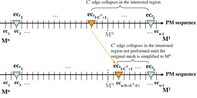
so, we will assure that there will be C∗ edge collapses in the interested region that are not yet performed after the original mesh is re-simplified to MN. This stage is illustrated in Figure 3.3.

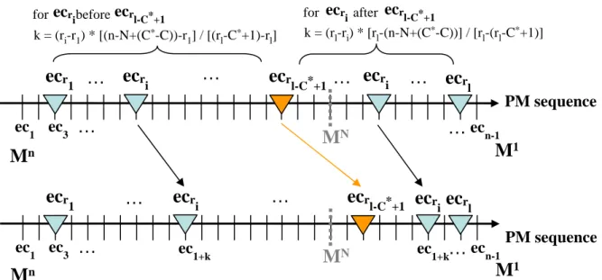
(b) Shift all edge collapses ecr1, ecr2,...,ecr(l−C∗),ecr(l−C∗+2),...,ecrl in a magnitude

similar to that for ecr(l−C∗+1). One way to do this is as follows:

• For each of ecr2,...,ecr(l−C∗), we shift ecri to the place for ecr1+k, where

k = (ri− r1) ∗ [(n − N + (C∗− C)) − r1]/[(rl− C∗+ 1) − r1].

• For each of ecr(l−C∗+2),...,ecrl, we shift ecri to the place for ecrl−k, where

k = (rl− ri) ∗ [rl− (n − N + (C∗− C))]/[rl− (rl− C∗+ 1)].

This stage is illustrated in Figure 3.4.

2. The new simplification cost for each of these shifted edge collapses ecr1,...,ecrl will

be the cost of the edge collapse at the shifted place. For example, if ecri is shifted

M

ec

ec

ec

…

…

M

…

M

M

ec

ec

…

ec

…

…

M

…

M

…

C*_{edge collapses in the interested region}

C*_{edge collapses in the interested}

region not performed until the original mesh is simplified to MN

Figure 3.3: Illustration of the first step in the weighting scheme.

Figure 3.5 depicts an example for the proposed weighting scheme, in which n is 36, N is 10, l is 8, C is 3 and C∗ is 5. In the first stage, we shift ecr4(= ecr(l−C∗+1)), marked

as the orange triangular dot, to the place for ec28(= ecn−N +(C∗_−C)). In the second stage,

all edge collapses ecr1, ecr2, ecr3, ecr5, ...,ecr8 are shifted as well. Take ecr2(= ec8) as an

example, the offset k coefficient is computed as (8 − 4) ∗ [28 − 4]/[20 − 4] = 4 ∗ 1.5 = 6, so its shifted place is at ec4+6 = ec10. Consider another example ecr7(= ec29), the offset

k is computed as (34 − 29) ∗ [34 − 28]/[34 − 20] = 5 ∗ 0.43 = 2, so its shifted place is at ec34−2 = ec32.

When the weighting is applied to more than one region simultaneously, the effect of weighting in each region would be less accurate because the shifted edge collapses for one region may conflict with the shifted edge collapses for another region. We take this issue into account in the re-simplification process. Once edge collapses ecr(l−C∗+1),...,ecrl are

shifted to appropriate places after the weighting scheme is applied in a region, they will not be performed in subsequent applications of weighting scheme in other regions unless the expected simplification target cannot be reached. When this happens, the prohibited edge collapses will be performed until the simplification target is reached.

3.2 Weighting Simplification Cost 25

M

ec

…

ec

ec

…

…

M

M

M

ec

M

ec

…

M

…

…

ec

…

ec

ec

…

…

ec

_…

ec

Figure 3.4: Illustration of the second step in the weighting scheme.

ec_r1 ec_r2 ec_r3 ec_r6 ec_r7 ec_r1 ec_r2 ec_r3 ec_r4ec_r5ec_r6ec_r7 ec_r8 ec 4 ec8 ec13 ec20 ec23 ec27 ec29 ec34 ec 4 ec10 ec17 ec28ec29 ec31ec32 ec34 M36 M10 M10 M1 M1 ec_r4 ec_r5 ec_r8 M36

3.3

Local Refinement

The basic concept of local refinement scheme is to locally refine the interested region by moving down along the active cut of the vertex hierarchy and in the mean time moving up along the active cut to keep polygon count fixed.

We mentioned the vertex splits dependency problem in section 2.4.1, which means that before doing a vertex split, several additional vertex splits may need to be executed due to dependency. Such behavior is not accepted for local refinement because more vertex splits lead to more edge collapses on other regions. In our implementation the vertex split dependency problem is resolved by strategies adapted from Kim’s approaches [13].

After local refinement, the costs on the refined regions are relatively lower, so during the subsequent local refinements the refined regions may soon be simplified. We shall adjust the costs on the refined regions to avoid such problem.

As shown in Figure 3.6, one way to avoid this problem is to level the cost distribution over the active cut such that costs assigned to those vertices newly splitted from a vertex v in the local refinement process to be above the cost of v. Moreover, it is desirable to preserve the difference in original costs for nodes in the subtree rooted at v.

To fulfill the above expectations, we prepare an collapse candidate list for each sub-tree rooted at some vertices splitted in the local refinement process, which enlists every executable edge collapses in the subtree. By leveling the costs of records in this list to be above the cost of the subtree’s root, the cost distribution over the active cut of the subtree can be leveled as well.

The collapse candidate list is updated only when a vertex is splitted from the root of the subtree, as follows:

• The corresponding edge collapse of this newly performed vertex split is inserted into the collapse candidate list.

• The edge collapse which collapses the vertex is removed from the collapse candidate list (if it exists in the list).

Afterwards, the costs of every edge collapse records in the collapse candidate list are updated as follows:

• Find the record with the smallest original cost among all the records in the list, denote this record as S.

3.3 Local Refinement 27

local−refined subtree

Cost

Active cut

Root node of the

(a) Active cut before local-refinement

The local−refined subtree

Active cut of the local−refined subtree

Cost

Active cut

(b) Active cut after local-refinement

Cost

Active cut

(c) Active cut after cost adjustment

Figure 3.6: The concept of our cost adjustment scheme. • Set the cost of S to be the cost of the subtree’s root.

• For other records in the collapse candidate list, we set the cost of recordi as the cost

of the subtree’s root + the difference of original cost between recordi and S.

Figure 3.7 demonstrates the changes of costs in the vertex hierarchy during the cost adjusting process. In Figure 3.7(a)) the vertex hierarchy before local refinements is shown, each box represent a vertex, and the number in it represent the cost of the vertex to be splitted (empty if the vertex is not splittable). In Figure 3.7(b), vertex #2 has just been splitted, and it will be the root of a new cost-adjusted subtree in the local refinement process. In Figure 3.7(c), vertex split #3 has just been executed, the collapse candidate list is updated by adding vertex split #3 into the list and remove vertex split #2 from the list, and the cost of vertex split #3 is set to be the cost of the root (70). In Figure 3.7(d), we first update the cost of the record with smallest original cost (vertex split #4)

as the cost of the subtree’s root (70), and update the cost of the other record (vertex . In Figure 3.7(e), Figure 3.7(f) and Figure 3.7(g), the costs of records in the cut list are adjusted using our cost adjusting scheme.

3.3 Local Refinement 29

#1 70

40

55 65

60 35

active cut of the vertex hierarchy #2

#3 #4

50

#5 #6 10 #7 30

(a) Before local refinement

#1 70 collapse candidate list: (#3,#4)Æ(#2) 40 55 60 35 70 #2 (65) #3 #4 50 10 #5 #6 #7 30

(b) After vertex #2 is splitted #1 70 collapse candidate list:

(#5,#8)Æ(#3) 40 55 70 35 70 #2 (65) 50 10 30 #3 #4 #5 #6 #7 (60) #8 #9 #10 #11 #12 #13 #14

(c) After vertex #3 is splitted

#1 70 collapse candidate list: (#5,#8)Æ(#3) (#6,#7)Æ(#4) 40 55 95 70 70 #2 (65) 50 10 30 #3 #4 #5 #6 #7 (60) (35) #8 #9 #10 #11 #12 #13 #14

(d) After vertex #4 is splitted #1 70

collapse candidate list: (#6,#7)Æ(#4) (#9,#10)Æ(#5) 40 55 95 70 70 #2 (65) 85 10 30 #3 #4 #5 #6 #7 (60) (35) (50) #8 #9 #10 #11 #12 #13 #14

(e) After vertex #5 is splitted

#1 70

collapse candidate list: (#9,#10)Æ(#5) (#11,#12)Æ(#6) 40 55 95 70 70 #2 (65) 110 70 30 #3 #4 #5 #6 #7 (60) (35) (50) (10) #8 #9 #10 #11 #12 #13 #14

(f) After vertex #6 is splitted #1 70

collapse candidate list: (#9,#10)Æ(#5) (#11,#12)Æ(#6) (#13,#14)Æ(#7) 40 55 95 70 70 #2 (65) 110 70 90 #3 #4 #5 #6 #7 (60) (35) (50) (10) (30) #8 #9 #10 #11 #12 #13 #14

(g) After vertex #7 is splitted

C H A P T E R

4

Experimental Results

In this chapter, experimental results of our works will be given. In the first subsections, we will perform tests for the weighting approach, and in the second subsection, tests for the local refinement approach are performed. In the third subsection, comparisons between weighting and local refinements are given. And in the last subsection, we will demonstrate using our two-staged approach to improve the quality of simplified meshes.

We use three models for testing, the first model is Armadillo with 10002 vertices and 20000 faces, which has surface details on some regions as well as some sharp features. The second model is Liberty with 17636 vertices and 35176 faces, which has one important sharp feature (the spikes on her crown) and surface details on some regions. The third model is Parasaur with 3870 vertices and 7685 faces, which has texture information. These models are shown in Figure 4.1.

(a) Armadillo (b) Liberty (c) Parasaur

Figure 4.1: The testing models.

All tests are performed on a PC with AMD Athlon 3000+ CPU and 512MB of RAMS and Geforce 6800 graphics card.

4.1

Weighting Tests

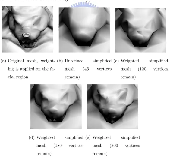
Figure 4.2 and figure 4.3 illustrates the result of the armadillo model simplified to 1, 000 polygons using different weighting conditions. The weighting is applied on the face of the armadillo model, and the remaining vertex count are 45, which is the unrefined case, 120, 180, and 300 vertices, as shown in figure 4.2(b)-(e), and figure 4.3 shows the quality of overall model. The effect of weighting is proportional to the number of remaining vertices in the weighted region, and the additional edge collapses on the unweighted regions are scattered evenly, so that the sacrifice of quality is barely visible. Table 4.1 lists the geometric errors of the unweighted and weighted simplifications relative to the original mesh. The errors are measured using Metro [2].

(a) Original mesh, weight-ing is applied on the fa-cial region (b) Unrefined simplified mesh (45 vertices remain) (c) Weighted simplified mesh (120 vertices remain) (d) Weighted simplified mesh (180 vertices remain)

(e) Weighted simplified

mesh (300 vertices

remain)

Figure 4.2: The quality improvement on weighted regions of Armadillo’s simplification. We also perform the above weighting tests on the simplification result of the Liberty model with 1000 faces, which are shown in Figure 4.4 and Figure 4.5, and similar results

4.1 Weighting Tests 33

(a) Unrefined simplified mesh, front (b) Weighted simplified mesh (120 vertices), front (c) Weighted simplified mesh (180 vertices), front (d) Weighted simplified mesh (300 vertices), front

(e) Unrefined simplified mesh, back (f) Weighted simplified mesh (120 vertices), back (g) Weighted simplified mesh (180 vertices), back (h) Weighted simplified mesh (300 vertices), back

Figure 4.3: The sacrifice of quality on unweighted regions of Armadillo’s simplification. global error local error

unweighted simplification 0.8156 1.6774

weighted simplification, remaining vertices = 120 0.8137 1.5785 weighted simplification, remaining vertices = 180 0.8513 1.5746 weighted simplification, remaining vertices = 300 1.0891 1.1065

Table 4.1: Comparing geometric errors of Armadillo’s weighted simplification with 2000 faces

are claimed. Table 4.2 lists the geometric errors of the unweighted and weighted simplifi-cations relative to the original mesh. The global error measures the geometric difference of the entire mesh and the local error focus on the regions where weightings are applied. The local error reduces when the remaining vertex count of weighted region increases while the global error arises. Since most of the errors are introduces to the regions we do not interested, and thus can be discarded.

(a) Original mesh, weight-ing is applied on the fa-cial region (b) Unrefined simplified mesh (10 vertices remain) (c) Weighted simplified mesh (60 vertices remain) (d) Weighted simplified mesh (180 vertices remain)

(e) Weighted simplified

mesh (360 vertices

remain)

Figure 4.4: The quality improvement on weighted regions of Liberty’s simplification.

global error local error

unweighted simplification 18.0879 1.6528

weighted simplification, remaining vertices = 60 18.0878 1.3043 weighted simplification, remaining vertices = 180 18.0877 0.8865 weighted simplification, remaining vertices = 300 18.0832 0.7985

Table 4.2: Comparing geometric errors of Liberty’s weighted simplification with 1000 faces

The effects of these three weightings will be blended to produce the final result. Regions without weighting can also be preserved well.

To find the effect of weighting on simplifications not at the weighting’s default simpli-fication ratio, we apply weighting on the facial region of Armadillo’s simplisimpli-fication with 1000 faces, then we generate simplifications at other ratios using the weighted PM se-quence. The testing results are shown in table 4.3, in which each row shows the number

4.1 Weighting Tests 35 of vertices on the selected region before and after weighting on simplification with a spe-cific simplification ratio, and comparisons between the unrefined simplifications and the simplifications generated from the above weighted PM sequence are shown in Figure 4.7. We find that effect of weighting is equally effective on simplifications with lower ratios then the default one (500 and 250 faces), but is less effective on simplifications with higher ratios (2000, 4000, 6000, 8000, 10000, 15000 faces).

face count vertices count before weighting

vertices count after weighting

increased vertices count respect to the face count

250 3 34 0.124 500 9 72 0.126 1000 (default) 17 148 0.131 2000 34 159 0.0625 4000 69 191 0.0305 6000 115 214 0.0165 8000 140 237 0.0121 10000 189 260 0.0071 15000 286 325 0.0026

(a) Unrefined simplified mesh, front (b) Unrefined simplified mesh, back (c) Weighted simplified mesh (60 vertices), front (d) Weighted simplified mesh (60 vertices), back

(e) Weighted simplified mesh (180 vertices), front (f) Weighted simplified mesh (180 vertices), back (g) Weighted simplified mesh (300 vertices), front (h) Weighted simplified mesh (300 vertices), back

4.1 Weighting Tests 37

(a) First weighting (b) Second weighting (c) Third weighting (d) Apply the three weightings simulta-neously

(e) First weighting ap-plied

(f) Second weighting ap-plied

(g) Third weighting ap-plied

(h) Three weightings ap-plied simultaneously

(a) simplification with 250 faces, weighted

(b) simplification with 500 faces, weighted

(c) simplification with 1000 faces (default), weighted

(d) simplification with 250 faces, unrefined

(e) simplification with 500 faces, unrefined

(f) simplification with 1000 faces, unrefined

(g) simplification with 2000 faces, weighted

(h) simplification with 4000 faces, weighted

(i) simplification with 8000 faces, weighted

(j) simplification with 2000 faces, unrefined

(k) simplification with 4000 faces, unrefined

(l) simplification with 8000 faces, unrefined

4.2 Local Refinement Tests 39

4.2

Local Refinement Tests

First we demonstrate the effect of cost adjustment for the cost distribution over the entire mesh in Figure 4.8. Figure 4.8(a) shows the original cost distribution over the entire simplified mesh of Armadillo with 1000 faces. In Figure 4.8(b) the cost distribution after local refinement but without cost adjusting is shown, and we can see that the local-refined regions (marked as red segments) have significantly lower cost than other regions. And Figure 4.8(c) shows the the cost distribution after local refinement with cost adjusting. We can see that with cost adjusting scheme the costs on the local-refined regions are leveled up to match the cost distributions over the entire mesh.

Cost

Active cut

(a) original cost distribution over the entire simplified mesh

Cost

Active cut

(b) cost distribution after local refinement without cost adjusting

Cost

Active cut

(c) cost distribution after local refinement with cost adjusting

Figure 4.8: The effects of cost adjusting for the cost distribution over the entire mesh.

Local refinement requires users to select a small region of surface mesh to be refined, and and the refine process is proceeded iteratively until satisfy. Figure 4.9 illustrates a small region of simplified mesh of 1, 000 faces with and without refined, and table 4.4 is the geometric error after each refinement iteration. The more iteration step, the better geometric features can be preserved, and affect less to the other regions than the weighting approach.

(a) The region to be refined on the orig-inal mesh

(b) Unrefined simplifi-cation

(c) After 1 iteration (4 vertex splits are performed)

(d) After 2 iteration (10 vertex splits are performed)

(e) After 3 iteration (18 vertex splits are performed)

(f) After 4 iteration (32 vertex splits are performed) (g) After 5 iteration (43 vertex splits are performed) (h) After 6 iteration (47 vertex splits are performed)

Figure 4.9: Using local refinement to gradually refine Armadillo’s left eye.

global error local error

unrefined simplification 1.3924 1.1964 after 1 iteration 1.3925 1.1203 after 2 iterations 1.3957 0.5284 after 3 iterations 1.3958 0.5338 after 4 iterations 1.3958 0.3578 after 5 iterations 1.3957 0.3515 after 6 iterations 1.3958 0.3521

Table 4.4: Geometric errors of performing local refinements on the left eye of the Armadillo model

approach, we show the locations of edge collapses executed by three consecutive local refinements with and without cost adjustments applied on the Armadillo model’s sim-plification with 1000 faces in Figure 4.10. The refined region of each local refinement is marked as red dots and the edge collapses executed by each local refinements are marked as green dots. We find that without cost adjustments, the refined regions of earlier local

4.2 Local Refinement Tests 41 refinements are likely to be collapsed by later local refinements, but with cost adjustments enabled the above problem is solved.

(a) First local refinement applied without cost adjustment

(b) Second local refinement ap-plied without cost adjust-ment

(c) Third local refinement ap-plied without cost adjustment

(d) First local refinement applied with cost adjustment

(e) Second local refinement ap-plied with cost adjustment

(f) Third local refinement ap-plied with cost adjustment

Figure 4.10: Edge collapses executed by local refinements with and without cost adjust-ments.

4.3

Comparisons of Weighting and Local Refinements

Both weighting and local refinement have their own strength and weakness, in this section, we will try to compare these two methods in several aspects.

Figure 4.11 demonstrates the simplification results of refining the facial region of Ar-madillo model’s simplification with 1000 faces using weighting, local refinements, and combining both methods, and table 4.5 lists the geometric error of Figure 4.11. Same numbers of vertices are added on the facial region by the three methods, for example, in Figure 4.11(a) 162 additional vertices are allocated by weighting, in Figure 4.11(b) 162 vertex splits are performed by local refinements, and in Figure 4.11(c) first 73 additional vertices are allocated by weighting, followed by 90 vertex splits performed by local re-finements. We find that the refining effect of weighting is concentrated on the selected region only, while the refining effect of local refinements tends to span across the selected region and effect the nearby unselected regions as well. This is because local refinement is based on the pre-built vertex hierarchy, so that to execute a vertex split on the selected region, more vertex splits may be executed due to parent-children dependencies in the vertex hierarchy. According to table 4.5, the refining effect of combining both methods is better then weighting and local refinements. The reason is that after weighting a better structured vertex hierarchy is formed, so the effect of local refinements could be more concentrated on the facial region, which results in less local and global errors.

global error local error

unrefined simplification 0.8018 1.4721

refined by weighting 1.2584 1.2214

refined by local refinements 1.4717 1.1045

refined by both 1.2583 0.7295

Table 4.5: Geometric errors on Armadillo’s refined simplifications by weighting, local refinements and both

We now compare the ability to recover sharp features using weighting and local re-finements. Figure 4.12 shows the results of using weighting to recover the spikes on the Liberty model’s simplification with 500 faces. Even we specify that all vertices on the spikes (marked as red dots in Figure 4.12(a)) shall remain after weighting, the shape of the sharp features is still not preserved well. On the other hand, the spikes can be recovered

4.3 Comparisons of Weighting and Local Refinements 43 after performing three iterations of local refinements on them, as shown in Figure 4.13.

In Figure 4.14 and Figure 4.15, results of using weighting and local refinements to recover the spikes on the Liberty model’s simplification with 1000 faces are shown. As shown in Figure 4.15, the spikes can be recovered after performing just one iteration of local refinement on them, with 7 additional vertices allocated on the refined region. But if we use weighting to recover the spikes with the budget of 7 additional vertices, the spikes cannot be recovered well, as shown in Figure 4.14(c). In fact, we have found that at least 11 additional vertices are required for weighting to recover the spikes, as shown in 4.14(d).

(a) Refined simplification by lo-cal refinements, facial region

(b) Refined simplification by weighting, facial region

(c) Refined simplification by

combining both methods,

facial region

(d) Refined simplification by lo-cal refinements, front

(e) Refined simplification by weighting, front

(f) Refined simplification by

combining both methods,

front

(g) Refined simplification by lo-cal refinements, back

(h) Refined simplification by weighting, back

(i) Refined simplification by com-bining both methods, back

Figure 4.11: Comparing the refined simplifications by weighing, local refinements and both.

4.3 Comparisons of Weighting and Local Refinements 45

(a) Weighted region on the origi-nal mesh.

(b) Unweighted simplification. (c) Weighted simplification.

Figure 4.12: Recover sharp features on the Armadillo’s simplification with 500 faces by weighting.

(a) Select vertices near the miss-ing spikes.

(b) Result after three iteration of local refinement.

Figure 4.13: Recover sharp features on the Armadillo’s simplification with 500 faces by local refinements.

(a) Weighted region on the origi-nal mesh.

(b) Unweighted simplification.

(c) Weighted simplification, 7 ver-tices are added on the weighted region.

(d) Weighted simplification, 11 vertices are added on the weighted region.

Figure 4.14: Recover sharp features on the Armadillo’s simplification with 1000 faces by weighting.

(a) Select vertices near the missing spikes.

(b) Result after one iteration of lo-cal refinements.

Figure 4.15: Recover sharp features on the Armadillo’s simplification with 1000 faces by local refinements.

4.4 Case Studies 47

4.4

Case Studies

In this section, we will demonstrate using our two-staged approach to refine the simplifi-cations of three different testing models.

4.4.1

Case1: Armadillo

In this subsection, we try to refine the simplification with 1000 faces of the Armadillo model produced by QEM using the proposed two-stage approach. We use weighting to improve the quality on the facial and torso regions and use local refinements to further refine the eyes. The comparisons between the original mesh, the unrefined simplification and the refined simplification are shown in Figure 4.16. In Figure 4.17, we can see the huge quality improvement on the facial and torso regions.

The geometric errors of the unrefined and refined simplifications are shown in table 4.6. While the global error increases after the refinement process because sacrifice of quality was done on unrefined regions, the local errors on the semantically important regions decrease considerably after refinement was applied.

global error local error unrefined simplification with 1000 faces 0.8018 2.4510

refined simplification with 1000 faces 1.1427 1.0239

(a) Original mesh (20000 faces), front (b) Unrefined simplification (1000 faces), front (c) Refined simplification (1000 faces), front (d) Original mesh (20000 faces), back

(e) Unrefined simplification (1000 faces), back

(f) Refined simplification (1000 faces), back

Figure 4.16: Comparison of the unrefined and the refined simplifications with 1000 faces of Armadillo.

Figure 4.17: Closer comparisons between the unrefined (left) and refined (right) simplifi-cations with 1000 faces of Armadillo.

4.4 Case Studies 49

4.4.2

Case2: Liberty

The second test case is the Liberty model’s simplification with 1000 faces produced by QEM. We use weighting to refine the face, torch and foots, and use local refinement to recover the spikes on the crown. The refined simplification and its comparison with the unrefined version and the original mesh are shown in figure 4.18.

Again we use Metro [2] to measure the geometric errors of the unrefined and refined simplifications, as shown in table 4.7. We find that there is no significant difference between the global geometric errors of unrefined and refined simplification, but the local errors on the refined regions are decreased.

global error local error unrefined simplification with 1000 faces 18.0879 4.4558

refined simplification with 1000 faces 18.0969 1.8194

(a) Original mesh (35176 faces), back (b) Original mesh (35176 faces), front (c) Unrefined simplifi-cation (1000 faces), back (d) Unrefined sim-plification (1000 faces), front

(e) Refined simplifica-tion (1000 faces), back

(f) Refined simplifica-tion (1000 faces), front

Figure 4.18: Comparison of the unrefined and the refined simplifications with 1000 faces of Liberty.

4.4 Case Studies 51

4.4.3

Case3: Parasaur

The third test model is Parasaur which has texture information. We choose APS as the simplification algorithm because it is designed for preserving textures, however, the texture quality of Parasaur’s simplifications still degrades notably when simplified to very low polygon counts, such as 500 faces. The comparisons between the original mesh, the unrefined simplification and the refined simplification are shown in Figure 4.19.

(a) Original mesh (3870 faces), left

(b) Unrefined simplification (500 faces), left

(c) Refined simplification (500 faces), left

(d) Original mesh (3870 faces), right

(e) Unrefined simplification (500 faces), right

(f) Refined simplification (500 faces), right

Figure 4.19: Comparison of the unrefined and the refined simplifications with 760 faces of Parasaur.