以考慮跳躍的信用市場模型定價信用衍生性商品

國立交通大學

財 務 金 融 研 究 所

碩士論文

以考慮跳躍的信用市場模型定價信用衍生

性商品

The Pricing of Single-Name Credit Derivatives by the

Credit Market Model With Jumps

研 究 生: 蔡呈偉

指導教授: 王克陸 博士

中華民國九十五年六月

以考慮跳躍的信用市場模型定價信用衍生性商品

The Pricing of Single-Name Credit Derivatives by the Credit

Market Model With Jumps

研 究 生: 蔡呈偉

ٛ ٛ ٛ ٛ

_{Student: Cheng-Wei Tsai}

指導教授: 王克陸博士

ٛ ٛ ٛ ٛ

_Advisor:

_Ph.D.

Keh-Luh Wan

國 立 交 通 大 學

ٛ

財

務

金

融

研

究

所

ٛ

碩 士 論 文

A Thesis

Submitted to Graduate Institute of Finance

National Chiao Tung University

in partial Fulfillment of the Requirements

for the Degree of

Master of Science

in Finance

June 2006

Hsinchu, Taiwan, Republic of China

中華民國九十五年六月

以考慮跳躍的信用市場模型定價信用衍生性商品

學生 : 蔡呈偉

指導教授: 王克陸 博士

國立交通大學財務金融研究所

2006 年 6 月

摘要

本文以一個考慮跳躍的信用市場模型定價信用違約交換(credit default swaps)與信 用違約交換選擇權(credit default swaptions)。本文提出一個跳躍擴散模型，將信用違約 交換的價差當作主要變數來計算信用違約交換選擇權的價格，其中跳躍的部份是以標點 過程(marked point processes)以及複合波式過程(compound Poisson processes)來描 述。藉著對跳躍部份的特別設定我們能夠推導出解析的定價公式。我們也提出兩個數值 的實例來顯示本模型的彈性：第一個是違約機率的計算，第二個是信用違約交換選擇權 的隱含波動度曲線之重製。

關鍵詞：信用市場模型，信用違約交換，跳躍擴散，標點過程，違約機率，隱含 波動度

The Pricing of Single-Name Credit Derivatives by the Credit

Market Model With Jumps

Student: Cheng-wei Tsai Advisor：Ph.D. Keh-luh Wang

Graduate Institute of Finance

National Chiao Tung University

June 2006

Abstract

This paper describes the pricing of credit default swaps (CDS) and credit default swaptions using market model with jumps. We propose a jump-diffusion credit market model that treats the CDS spread as the major variable to value a credit default swaption, in which the jumps are modeled by the marked point processes (MPPs) as well as the compound Poisson processes. Analytic pricing formula exists under some appropriate specification on the jump part of the CDS spread dynamics. We also make two numerical illustrations to show the flexibility of this model: The first one is the calculation of default probability and the second one is the reproducing of implied volatility curve for credit default swaptions.

Keywords: credit market model, jump-diffusion, CDS, marked point process, default

Acknowledgement

首先感謝父母多年來的教養與培育，在我求學的路途中給予持續不斷的鼓勵 與支持，讓我得以無後顧之憂的在學校追求學問，並完成研究所的學業。接下來 我要感謝研究所之指導教授王克陸博士於我撰寫論文期間的教導。從論文題目， 論文架構，模型假設，乃至於結果之推導與解釋，王教授皆給予相當多有效且負 建設性的建議，讓我能夠完成一篇頗具水準的碩士論文，並順利獲得碩士的學 位。最後感謝其他在我就讀研究所過程中曾經給予我任何幫助的師長，與所有陪 伴我一起渡過研究所生涯之同學，共同奮鬥所收穫的果實是最甜美的。

Content

1.

Introduction...1

2.

Model Settings and Review of Credit Market Model...3

2.1 Notations:...3

2.2 Some Important Relationships: ...4

2.3: A Brownian-motion-based Credit Market Model...5

3.

An Extension to Jump-diffusion Process ...5

3.1 Model Pre-settings: Jumps in Two Forward Rates...5

3.2 Modeling with the Marked Point Processes ...7

3.3: Constructing jump processes from MPPs ...9

3.4: Modeling with the Compound Poisson Processes ...10

4.

Pricing Credit Default Swaps and Swaptions ...11

4.1 Credit Default Swaps ... 11

4.2: Pricing Credit Default Swaptions...13

5.

Numerical Illustrations...18

5.1 Default Probability and Survival Curve ...18

5.2 Implied Volatilities of Credit Default Swaptions...22

6. Conclusion ...24

References...26

Appendix A – Change of measure with the inclusion of jumps...28

1. Introduction

The blooming credit derivative market has rendered numerous market practitioners and scholars focusing their attentions on credit models. The research in credit risk modeling was pioneered by Black and Scholes (1973) and Merton (1977), who take the firm value as a latent variable and defined the credit event based on the firm value, and this kind of models is categorized as the structural form model. The other sort of credit model is called the reduced form model, or intensity model, which models the default intensity process and assumes the default time to be random (Jarrow and Turnbull (1995), Lando (1998), etc).

In this paper, we model the discrete, simply compounded riskfree and risky forward rates and use the observable CDS spread to value the credit default swaption. Ever since Brace, Gatarek and Musiela (1997) developed the Libor Market Model (LMM), it has been used by market practitioners as a standard method to model the discrete compounded, market quoted forward rates. Due to the popularity of market models in the interest rate market, some scholars are applying the market model for the credit risk problems. Schönbucher (2000) takes the forward credit spread, the difference between the risky forward rate and the riskfree forward rate implied by the bond market, as a major variable and deduces the dynamics of CDS spread and the price of credit default swaption. Jamshidian (2002) introduces a numeraire–invariant approach in pricing default swaptions and derives a new formula on fractional recovery of pre-default contract value. Bennani and Dahan (2004) price the credit default swaptions in an equivalent risk neutral measure by imposing the default accumulator process that contains default time information. Brigo (2004) obtains a joint dynamics of CDS spreads under a single probability measure, and derives an approximated no-arbitrage valuation formula for constant term credit default swaps. Wu (2005) develops a new credit market model in which recovery rate is no longer an exogenously given input. The most crucial setting in the paper is his definition on defaultable zero coupon bonds which are backed by the coupons of corporate bonds. In that way, the pricing numeraire becomes tradable and CDS can be replicated by the defaultable bonds and annuities.

A common feature of the above credit market models is the assumption of the geometric Brownian motion for the underlying asset. Although simple and tractable, this naive setting yields unreasonable financial implications: it cannot describe properly the leptokurtic and asymmetric feature of the distribution of asset returns. The first to apply jump-diffusion model in asset pricing is Merton (1976). As investigated by Bystrom (2005), the distribution of CDS spread returns is much more leptokurtic and skewed than that of stock returns. Figure 1.1 illustrates the historical path of some entity’s CDS spreads and exhibits the leptokurtic and asymmetric

distribution of its spread returns. The empirical study of Jorion and Zhang (2005) examines credit events by using jumps in CDS market, suggesting that drastic upward jumps in CDS spreads reflect unanticipated credit events. Other than the lognormal distribution, we embed jump processes on the dynamics of those underlying variables. There are several reasons why jumps should be included in pricing credit derivatives. First, the ranges of the market quoted CDS spreads are too wide for the pure-diffusion lognormal model to fit. Secondly, big drops in price of a financial asset often occur due to sudden unexpected events, especially for financial contingents related to credit risk. For example, the corporate bond value has a tendency to plunge when default event occurs, which pushes up its defaultable forward rate and credit spread. Thirdly, with the inclusion of the jump process our model has ability to explain various credit derivatives market phenomena, such as the leptokurtic distribution of CDS spreads and the volatility smile in credit default swaption.

We suppose that both the defaultfree forward rate and the defaultable forward rate are described by the geometric Brownian motion plus some jump parts. This preliminary setting will make other variables such as credit spread, hazard rate, and CDS spread jump-diffusion processes. In addition to derive the pricing formulae of credit default swaps and swaptions, we will plot the implied volatility curves of swaptions and demonstrate the flexibility of this jump-diffusion model in reproducing multiple shapes of implied volatility. The price of credit default swaption attained in this model has an excellent explanatory power for the volatility smiles and skews of the instrument. Moreover, this model can forecast the widening of CDS spread and explain the shift of the survival curve.

The rest of this paper is arranged as the following: In section 2 we review the diffusion version of the credit market model. Section 3 introduces the jump-diffusion credit market model characterized by the compound Poisson processes. In section 4 we price some single-name credit derivatives, including CDS and option on CDS spread. Several numerical results are illustrated in section 5, including the default probability, the survival probability stripped from CDS quotes, and the implied volatility of credit default swaptions. Finally, we conclude in section 6.

Figure 1.1 Left: Historical path of General Motor’s CDS spreads; Right:

The distribution of General Motor’s CDS spread returns.

2. Model Settings and Review of Credit Market Model

In this section we review the market model in credit risk introduced by Schönbucher (2000) and build up some preliminary model settings.

2.1 Notations:

Here we assume all the cash flows occur at discrete tenor time:

0 1

0≤T ≤ ≤ ≤T ... T_m , and assume a common length of time interval:

1

: _k T_k T_k, k 0,1,...m 1

δ δ= = ₊ − ∀ = − ,

And τ is a stopping time, which is the time at which a credit event occurs.

U

Bond Prices:

The default-free (riskfree) zero-coupon bond price at time t with maturity T is _k

( , _k) _k( )

B t T ≡B t .

The defaultable zero-coupon bond (or the so-called corporate bond) price at time t with maturity T is _k

( ) ( , _k) ( ) _k( )

I t B t T ≡I t B t , where

I (t )= 1_{{τ >t}}is an indicator function representing the survival event until time t .

{τ >t} is the event that no defaults happen at and before time t .

U

Forward rates:

We then set the default-free forward rate（or simply forward Libor rate） implied by riskfree bond prices to be

(2.1) L_k(t )= L(t;T_k, T_{k+ 1}) @1 δ ( B_k(t ) B_{k+ 1}(t ) − 1) , and defaultable forward rate implied by defaultable bond price is

(2.2) L_k(t ) = L (t;T_k, T_{k+ 1}) @1 δ ( B_k(t ) B_{k+ 1}(t ) − 1) . The forward credit spread is defined as

(2.3) S_k @L_k−L_k

The defaultfree annuity

(2.4) B_m,n(t)= δB_k+1(t)

k= m n−1

∑

(2.5) B_m,n(t)= δB_k+1(t) k= m

n−1

∑

The above two annuities, which accumulate each single-period bond value in a given interval, are used as discount factors in this model.

The default risk factor:

(2.6) k k k B D B @

The quantity D t has a significant financial implication. ( )_k( ) I t D t is shown _k( ) by Schönbucher (2000) to be the conditional survival probability of the underlying entity under the P_k − forward measure. That is,

(2.7) ( )I t D t_k( )=P_k(τ >T_k|F_t), and

(2.8) D_k(0)=P_k(τ >T_k),∀ =k 0,1,...m−1.

Therefore (0)D_k can be regarded as the survival curve. Next, we define the forward default intensity (or discrete-tenor default intensity)

(2.9) 1 1 ( k 1) k k D H D δ + − @ .

Schönbucher (2000) also verified that (2.10)

1

δ(1− Dk+1(Tk))→ Hk(Tk) as δ→ 0.

Hence, H can be interpreted as the default probability for the next infinitesimal _k

small time step, which is called the instantaneous forward default probability. Besides its meaningful implication in finance, this variable also plays a crucial role in the later-on model derivation. H is also named as hazard rate in some literatures. _k

2.2 Some Important Relationships:

The followings are some important relationships between the above notations. Relationship of forward rates and bond prices:

(2.11)

B_k(t)

B_k+1(t)= 1+δLk(t)

Let ( )η t =inf{i≥0 :T_i≥ , then t} (2.12) 1 ( ) ( ) 1 ( ) ( ) 1 ( ) k k t j t j B t B t L t η η δ − = = +

∏

, 1 ( ) ( ) 1 ( ) ( ) 1 ( ) k k t j t j B t B t L t η η δ − = = +

∏

And (2.13) 1 ( ) ( ) 1 ( ) ( ) 1 ( ) k k t j t j D t D t H t η η δ − = = +

∏

(2.14) Sk = +(1 δL Hk) k

Relationship of forward default intensity and forward rates： (2.15) (1+δL_k)= (1 +δL_k)(1+δH_k) H_k = 1 δ( 1+δL_k 1+δL_k − 1)

2.3: A Brownian-motion-based Credit Market Model

They assume that both forward rates are driven by geometric Brownian motions. In the following we specify the dynamics of the fundamental variables under the

1

k

T ₊ -forward default measure, which is defined in the following.

2.3.1: Definition (The Survival Measure)

A T -forward default measure _k P_k is a probability measure, under which any asset taking the defaultable bond price B_k as a numeraire is a martingale.

Dynamics of two forward rates:

dL_k(t)

L_k(t−)=γk(t)dWk+1(t),

dL_k(t)

L_k(t−)=γk(t)dWk+1(t)

Dynamics of forward credit spread and default intensity:

dS_k(t) S_k(t−)=γk S (t)dW_k+1(t), dH_k(t) H_k(t−)=γk H (t)dW_k+1(t)

These dynamics are owing to the assumption that risk-free interest rate and default intensity are independent. Schönbucher (2000) verifies that with this independence setup all the fundamental variables, including risk-free and risky forward rates, forward credit spread, and forward default intensities, are all martingales under the forward default measure under which assets taking the defaultable bond as numeraires are martingales. Brigo and Alfonsi (2003) provide evidence that correlation between interest rate and credit spread (or default intensity) has little effect on CDS prices. Independence assumption between riskfree rates and defaults can facilitate model derivation.

3. An Extension to Jump-diffusion Process

3.1 Model Pre-settings: Jumps in Two Forward Rates

We first specify the jump-diffusion dynamics of defaultfree and defaultable forward rates. Glasserman and Kou (2003) incorporate the jump-diffusion in the term structure of simple compounded forward rate, proposing a “jump version” of Libor

market model. However, jumps in both defaultfree and defaultable forward rates are more complicated. When riskfree rate jumps, odds are high that risky rate would have a jump simultaneously. It may reflect changes in some macroeconomic conditions such as recessions, which could be regarded as part of the systematic risk. Jumps in the risky rate could reflect the non-systematic risk like the credit standing of a company. The value of the corporate debt has a tendency to drop if the company is alleged to have some financial crisis, or suffers from a down-grade in its credit rating. This will in turn cause an up-jump in the forward rate of its defaultable bond.

3.1.1 Dynamics of forward rates and spreads

The followings are the jump-diffusion dynamics of the forward rates: for defaultfree forward rates,

(3.1) dL_k(t ) L_k(t−) =γk(t )dWk+1(t )+ d %Jk L (t ),

and for defaultable forward rates,

(3.2) dL_k(t ) L_k(t− ) =γk(t )dWk+1(t )+ d ( %Jk L (t )+ %J_kL (t )),

with the compensated jumps %Jk L (t )= J_kL(t )− EJ_kL(t ) and %J_kL (t )= Jk L (t )− EJk L (t ), where J_kL (t)= L_k(s)− L_k(s−) 0<s≤t

∑

= ∆L_k(s) 0<s≤t

∑

, and J_kL (t)= L_k(s)− L_k(s−) 0<s≤t

∑

= ∆L_k(s) 0<s≤t

∑

.

We can see that the defaultfree forward rate is driven by the single jump, L k

J% , representing the systematic risk. The defaultable forward rate is affected by two types of jumps with the first one ( L

k

J% ) induced by the macroeconomic conditions, or the systematic risk, and the second one ( L

k

J% ) by the credit standing of the underlying entity. We impose the independence assumption noticed in section 2.3 on these two types of jump risks.

The dynamics of forward default intensity H and credit spread S under the survival measure can be expressed as:

(3.3) dH_k(t) H_k(t−)=γk H dW_k+1(t)+ d %J_kH(t) (3.4) dS_k(t ) S_k(t−) =γk S dW_k+1(t )+ d %J_kS (t ).

Applying Ito’s Lemma, the following relationships specify the volatility and jump terms of H in terms of two forward rates, _k

(3.5) γk H (t )= Lk(t− )γk(t )− Lk(t− )γk(t ) L_k(t− ) − L_k(t− ) , J_kH (t )= Lk(t− ) L_k(t− ) − L_k(t− ) ∆Lk(s) 0< s ≤ t

∑

+ Lk(t− ) L_k(t− ) − L_k(t− ) ∆Lk(s) 0< s ≤ t

∑

+ δLk(t− ) 1+δL_k(t− )0< s ≤ t

∑

∆Lk( s) 2 +δ 2 L_k2 (t− ) L_k(t− ) L_k(t− ) − L_k(t− ) 0< s ≤ t

∑

∆Lk(s) 3

The cubic term, which is considerably small, can be neglected. Therefore, the jump part of the forward default intensity can be decomposed as:

(3.6)

J_kH_(t)

= C₁× Jump of defaultable forward rate +C₂× Jump of defaultfree forward rate +C₃× (Jump of defaultfree forward rate)2

for some constants C₁,C₂,C₃.

(3.6) reveals that jump effects of both defaultfree and defaultable forward rates would contribute to the jumps of forward default intensityH , with first order in jump magnitude of L and first order plus second order in jump magnitude of L . Jumps in forward default intensity are due to jumps in riskfree rate and risky rate, but jumps in riskfree rate would impact forward default intensity more than jumps in risky rate do. In the case of forward credit spread S, the relationships ( S

k

γ and S k

J%) can be derived in the same way by Ito’s Lemma, and S

k

J% can be decomposed similarly as the above. Jumps in defaultfree and defaultable forward rates would give rise to jumps in forward credit spread as well. The difference is that jumps in riskfree rate and jumps in risky rate contribute equally to forward credit spread S.

By using Ito’s Lemma, we can also derive the dynamics of HBkB in terms of riskfree forward rate and credit spread:

(3.7) dHk(t) Hk(t−) = [ δ2Lk(t−) 2 (1+δLk(t−)) 2γk 2 − δ (1+δLk(t−)) 2γkγk S ]dt+ (γk S₋ δLk(t−) 1+δLk(t−) γk)dWk+1(t) _+dJ%_kS(t ) .

3.2 Modeling with the Marked Point Processes

Thanks to the succinct decompositions of jump terms in section 3.1, we are able to detect the influences of jumps in forward rates on the hazard rate and credit spread. Nevertheless, the jump part in expression (3.1) or (3.2) is not specific enough to be an effective mathematical representation. To build a pricing model we have to rely on a more solid and sound theoretical framework. As Bjork et al. (1997) models the continuous short rate by MPPs and Glasserman and Kou (2003) uses MPPs to explain

jump risk in riskfree forward rate, we are going to model the jumps of each forward rate by imposing a class of stochastic processes, the Marked Point Process (MPP), and scrutinize the insight of the jump model in this general framework. We shall first briefly introduce the definition of the marked point processes.

3.2.1: Definition (Marked Point Process)

Consider a filtered probability space(Ω, F,{F}_t, P). A marked point process is meant by a pair of sequence {T_n,X_n}_n≥1, with the point T_n increasing and T_n → ∞ as

n→ ∞ almost surely, and the mark Xn is adapted, taking values on any abstract space E.

Although the marks may in general take values in any abstract space, it suffices to consider the non-negative real-valued marks. Tn is a sequence of time point at which there is an occurrence of the mark Xn. When it talks to construct a jump process by MPPs, we need to define a function of the mark and point, namely,h(Tn,Xn). The function h maps the mark Xn from an abstract space into a real value. The jump process is to be formulated as the sum of function h:

(3.7) = =

∑

1 ( ) ( , ) t N i i i J t h T X ,

where N_t is a counting process which counts the number of marks before time t .

Let µ([0,t ]× A) be a random measure counting the number of occurrence of the pair

(T_n,X_n) within time interval [0,t] with X_n in A, namely, µ([0,t ]× A) = #{i :Ti ∈[0,t], Xi ∈A}.

Note that µ is a positive integer-valued measure and is finite for every bounded set A. Hence, the jump process can also be expressed as an integral with respect to the counting measureµ : (3.8) J (t) = h(s, x) [0,t ]× E

∫

dµ(s, x) , with (3.9) × =

∫

[0, ] ( ( )) ( , ) ( , ) t E E J t h s x dv s x ,

where v is called the intensity measure of the MMP. Furthermore, we require the following compensated version of the jump process, which is important in pricing financial contracts: (3.10) µ × × =

∫

−

∫

% [0, ] [0, ] ( ) ( , ) ( , ) ( , ) ( , ) t E t E J t h s x d s x h s x dv s x .

Note that such a process is a martingale. Later on the dynamics of every variable will be expressed as a diffusion term plus a compensated jump process so that it would retain the martingale property.

There are sufficient reasons why the marked point process is an appropriate candidate to be applied in this pricing model, the most important among which is that the jump intensity and distribution of jump magnitude may not be preserved under change of measure. Glasserman and Kou (2003) pointed out that even if jumps are presumed to be Poisson in one measure, we must suppose them to follow marked point process in other measures.

3.3: Constructing jump processes from MPPs

Our next attempt is to re-specify the dynamics of forward rates with the MPP introduced earlier. dL_k(t ) L_k(t−) =γk(t )dWk+1(t )+ d %Jk L (t ) and dL_k(t ) L_k(t−) =γk(t )dWk+1(t )+ d ( %Jk L (t )+ %J_kL (t ))

are respectively the jump-diffusive dynamics of defaultfree and defaultable forward rates. Therein, we consider the compensated jump processes described in the previous subsection: (3.11) %JL (t )= hL(s, x) [ 0,t ]× E

∫

dµL(s, x)− hL(s, x) [ 0,t ]× E

∫

dvL(s, x) = hL (T_i, X_i) i=1 Nt

∑

− hL (s, x) [ 0,t ]× E

∫

dvL (s, x), and (3.12) %JL (t )= hL(s, x) [ 0,t ]× E

∫

dµL(s, x)− hL(s, x) [0,t ]× E

∫

dvL(s, x) = hL(T_i, X_i) i=1 N_t

∑

− hL(s, x) [0,t ]× E

∫

dvL(s, x)

Sometimes it is more favorable for us to have the jump of defaultable forward rate represented as a single term. For this reason, the two jumps in L are merged into one jump.

First we define two sets, which respectively describes the events that a jump occurs on riskfree and defaultable forward rate,

A(s)= {s | ∆Lk(s)≠ 0}, A(s)= {s | ∆L_k(s)≠ 0} . The merged jump term is

(3.13) J_k*(t)= J_kL(t )+ J_kL(t )= h_kL(T_i, X_i) i=1 N_tk

∑

+ h_kL(T_i, X_i) i=1 N_tk

∑

= h_k*(T_i, X_i) i=1 N_t*k

∑

, where N t *k

is the Poisson process associated with the jump J_k*

(t ) . (3.14) N t *k = N t k+ N t k − 1_{A( s )∩ A(s)} 0<s≤t

∑

, and (3.14) h_k*(T_i, X_i)= 1_A(T i)hk L (T_i, X_i)+ 1_{A (T} i)hk L (T_i, X_i)

3.4: Modeling with the Compound Poisson Processes

Though the generalized setting of marked point process contributes to a comprehensive and constructive mathematical approach, it is somewhat abstract and difficult to be implemented in practice. We are going to restrict the big framework to a more specific class, in which jumps of forward rates are assumed to be the compound Poisson processes made up of jump times and jump magnitudes. The compound Poisson process possesses information of “when the jump occurs” and “how large the jump is.”

3.3.1: Definition (Compound Poisson Processes)

A compound Poisson process (CPP) takes the form

J (t)= ( X_i

i=1 N_t

∑

− 1),

where N is a Poisson process that counts the jump times from time 0 to time t _t

with mean jump rate λ , and the random variable X is i.i.d. with some _i

density.

Xi − 1 denotes the jump magnitude as a fraction of the i-th jump.

A marked point process in which the points follow a Poisson process, the marks are i.i.d. random variables and the function h is represented as h(T_i,X_i)= X_i− 1is a compound Poisson process. The intensity measure of X can be written as

(3.15) v dt dx( , )=λf dx dt( )

Expression (3.15) enables us to calculate an integral with respect to the intensity measure in the particular compound Poisson case:

h(s, x)

∫

v(ds, dx)= (x °×[0,t ]

∫

− 1)λf (dx)ds =λ⋅ (x − 1) f (dx) °

∫

⋅ ds 0 t

∫

=λmt

Hence, we have the compensated compound Poisson process

(3.16) J t%( )=J t( )−λmt.

The followings are the specifications of compound Poisson dynamics of the forward rates, (3.17) % J_kL (t)= J_kL (t)−λ_km_kL t= (Y_{k ,i}L i=1 N_tk

∑

− 1) −λ_km_kL t, E(Y_{k ,i}L − 1) = m k L , (3.18) % J_kL (t)= J_kL (t)−λ_km_kL t= (Y_{k ,i}L − 1) i=1 N_tk

∑

−λ_km_kL t, E(Y_{k ,i}L − 1) = m k L

The jump magnitudes can be arbitrarily distributed, but attaining a closed-form swaption pricing formula requires a specific setting on the jump size distributions. The jump part of H is _k

(3.19) % J_kH(t ) = J_kH(t )− λ_kHm_kHt = (Y_{k , i}H i= 1 NtH k

∑

− 1) − λ_kH m_kHt , where N t Hk = N t k + N t k− 1_{A( s )∩ A(s)} 0

∑

< s≤t , and m_kH = E(Y_{k ,i}H − 1).

Note that the expression of Poisson process of H makes sense because either a _k

jump in riskfree forward rate or in defaultable forward rate will cause a jump in the forward default intensity.

4. Pricing Credit Default Swaps and Swaptions

4.1 Credit Default Swaps

In this subsection we are going to determine the fair “spread” or “premium” of a CDS contract.

4.1.1: Definition (Credit Default Swap)

A Credit Default Swap is a financial contract that allows the buyer to gain default protection from the seller by paying a periodical premium in exchange for

compensation on loss of the underlying credit. If default occurs between tenor time

[Tk−1,Tk], the compensation paid by the protection seller will be postponed to Tk. The premium, called CDS spread, could be either fixed or variable over the contract life. For the sake of simplicity we would assume the CDS spread to be a constant, S. To

analyze the cashflow stream of a CDS, we shall introduce the two separated parts of a CDS, which are the fee leg and the protection leg. Suppose the CDS contract is signed at start date T_m and matures at maturity date T_n, then the time-t value of the fee leg in terms of basis points proportional to the tenor length is

(4.1) 1 , ( ) 1( ) n m n k k m S t δB t − + =

∑

;

while the protection leg paid by the protection seller as long as default occurs is defined as (4.2) 1 1 1( ) [(1 )1{k k }] (1 ) ( ) n k t T T k k m B t E R _τ R e t + − + < ≤ = − = −

∑

,

where ( )e t denotes time-t value of 1 dollar at _k T_k+1 if default occurs in the interval

[Tk,Tk+1], and R is the recovery rate. Some literatures refer 1− R to Loss Given

Default (LGD). e could be written as _k B_k+1(t)E_t[(1− R)1_{T

k<τ ≤Tk+1}] which was proven by

Schönbucher (2000) and also mentioned by Bannani and Dahan (2004).

4.1.2: The Fair CDS Spread

The value of a CDS contract is the difference of the fee leg and protection leg

1 1 , ( ) 1( ) 1( ) (1 ) ( ) n n m n k k k k m k m S t δB t B t R e t − − + + = = − −

∑

∑

.

The fair CDS spread is attained by equating the fee leg and protection leg of a CDS. As a consequence the CDS spread is valued to be

(4.3) S_m,n(t) @ B_k+1(t) k= m n−1

∑

E_t[(1− R)1_{T k<τ≤Tk+1}] δB_k+1(t) k= m n−1

∑

= (1− R) e_k k= m n−1

∑

δB_k+1(t) k= m n−1

∑

Furthermore, some notational computations yield

(4.4) e_k k= m n−1

∑

δB_k+1(t) k= m n−1

∑

= δB_k+1(t) k= m n−1

∑

H_k(t) B_m,n(t) ,

so the CDS spread could be represented as (4.5) S_m,n(t)= α_k+1(t) k= m n−1

∑

H_k(t), where αk+1(t)= 1 1 1 , 1 ( ) ( ) (1 ) (1 ) ( ) ( ) k k n m n k k m B t B t R R B t B t δ _{+ +} − + = − = −

∑

.

The expression (4.5) is a useful relationship enabling us to link CDS price and default probability through weighted average, which is analogous to what we have seen in interest rate swap pricing from the Libor market model. This formula makes the separation of CDS quotes and survival probabilities (also default probabilities) possible, though just for the case that independence between interest rate and defaults is assumed. Recall that H t is the discrete tenor hazard rate: _k( )

1 1 ( k 1) k k D H D δ + = − ,

and that the default probability is just the ratio of defaultable bond price to defaultfree bond price. Hence the expression of CDS spread in (4.5) is linked to default probability which can be determined without any information of defaultable bonds. The details are left in section 5. A closed-form pricing formula of credit default swaption will be obtained by manipulation of equation (4.5) and change of measure. Due to the jump-diffusion setting here, the pricing formula is supposed be similar to that of interest swaption in Glasserman and Kou (2003), which takes the form of an infinite series, composed of Black-Scholes option formulae.

4.2: Pricing Credit Default Swaptions

4.2.1: Definition (Credit Default Swaption or Credit Spread Option)

sign a CDS contract with a predetermined spread S （”the strike price”）* . Assume the swaption starts at time 0 and terminates at timeT . The payoff of a payer credit swaption at maturity T ≤T_m is [(S_m,n(T ) δB_k+1(T ) k= m n−1

∑

− (1− R) e_k k= m n−1

∑

(T ))− (S * δB_k+1(T ) k= m n−1

∑

− (1− R) e_k k= m n−1

∑

(T ))]+ = δB_k(T ) k= m n−1

∑

× [S_m,n(T )− S*]+

Similarly, the payoff of a receiver credit swaption at maturity is

δB_k(T )

k= m n−1

∑

× [S * −S_m,n(T )]+

Since it can be considered as an option on CDS spread, the credit default swaption is also named as Credit Spread Option (CSO).

Note: Hereafter all the cases of credit default swaptions we consider are payer-type

swaptions.

As our goal is to price a credit default swaption, we will change the original probability measure to another one called the default swap measure, or forward survival measure as applied by Schönbucher (2000) and Bennani and Dahan (2004). The definition of a default swap measure is given as the following.

Definition 4.2.3 (Default Swap Measure)

The PBm,nB - default swap measure is a probability measure, under which any security taking the defaultable annuity B_{m n,} as a numeraire is a martingale.

Manipulating change of measure requires the application of Girsanov theorem. However, while change of measure with respect to a geometric Brownian motion only makes the drift term altered, change of measure in a jump-diffusion model will simultaneously yield different jump parameters. In this model change of measure will also lead the jump intensity and jump size mean and volatility to change. Bjork et al. (1997) proved a generalized version Girsanov theorem to deal with jumps in underlying variables, which is restated in the following.

Theorem 4.2.4 (Girsanov)

Consider a filtered probability space(Ω, F,{F}_t, P) . Let W (t ) be a standard Brownian motion and θ(t ) a predictable process such that

|θ(s) |

0

t

If we define a process Z such that

(4.6) dZ(t)= Z(t)θ(t)dW (t)+ Z(t−) (Φ(t, x) − 1){µ(dt, dx) − v(dt,dx)}

E

∫

,

where Φ(t, x) is a process satisfying

|Φ(s, x) |λ(s, dx) E

∫

0 t

∫

ds< ∞ , and EPZ (t )= 1,

then there exists a measure Q equivalent to P with

Z(t )= dQ

dP(t )

such that

dW (t) =θ(t )dt+ d %W (t ) , where %W (t ) is a standard Brownian motion under Q,

and the jump intensity under Q is (4.7)

vQ(t, dx)= Φ(t, x)vP(t, dx)

Glasserman and Merener (2003) give a thorough mathematical procedure on how to derive the function Φ , and the details are restated in appendix A. Rewrite (4.6) in integral form we have

(4.8) Z(t )= exp{ [−1 2θ(s) 2 ds+θ(s)dW (s)+ (1 − Φ(s, x))v(ds,dx) E

∫

] 0 t

∫

+ ln i=1 Nt

∑

Φ(T_i, X_i)} . Where the function Φ is

( ) 1 ( ) ( , ) 1 ( )(1 ) k n j k k m j t j L t t x b L t x η δ δ = = + Φ = + +

∑ ∏

, where b_k = Bk+1(t) δB_k+1(t) k= m n−1

∑

= B_k+1(t) B_m,n(t)

4.2.5 The dynamics of forward CDS spread

Before deriving the swaption pricing formula, the process of a forward CDS spread needs to be specified. From definition (4.2.3) we can inferred that a CDS

spread is a martingale under the associated default swap measure. Hence by martingale representation theorem, the process of spread SBm, nB (t) can be expressed in the following differential form

(4.9) dS_m,n(t) S_m,n(t−)=γm,n(t)dWm,n(t)+ d %Jm,n(t), where (4.10) d %Jm,n(t)= hm,n(Ti, Xi) i=1 N_t

∑

− hm,n(s, x 0 ∞

∫

)dvm,n(s, x) 0 t

∫

, or in integral form (4.11) S_m,n(t )= S_m,n(0)⋅ exp{ [−1 2γm,n(s) 2 ds+γ_m,n(s)dW_m,n(s) 0 t

∫

− hm,n(s, x)dv m,n (s, x) 0 ∞

∫

]+ ln i=1 N_t

∑

(hm,n(Ti, Xi)+ 1)} .

In the compound Poisson setting we are able to derive a closed-form swaption pricing formula as long as the distribution of jump magnitude is appropriately assumed. Glasserman and Kou (2003) assume the jumps to be lognormally distributed, while Kou (2002) uses double exponential distribution to describe the jumps. Here we will apply the lognormal assumption on the jump distribution.

Assumption 4.2.5 We assume Yi

m,n

is lognormally distributed with mean 1+ m_Y

and log-volatility s, and lnYi m,n : N (ln(1+ mY)− 1 2s 2 , s2). Therefore, in the particular compound Poisson case we have (4.12) S_m,n(t )= S_m,n(0)⋅ exp{ [−1 2γm,n(s) 2 ds+γ_m,n(s)dW (s) 0 t

∫

]−λ_m,nmt + ln i=1 N_t

∑

(Yi m,n )} .

Where we replace h_m,n by Y_im,n− 1, which is the jump magnitude of S_m,n as a

fraction of S_m,n.

4.2.6 Value of a credit default swaptions

Denote C(t,T_m,T_n, S*) by the time-t value of a payer credit default swaption providing the buyer enter into a CDS contract starting at T_m and terminating at T_n

with the strike spread S*. The swaption’s payoff at the maturity T is

C(T ,T_m,T_n, S*)= δB_k(T ) k= m

n−1

By the definition 4.2.3 we know that the CDS spread is a martingale under the default swap measure. Hence, via operation of conditional expectation under PBm,nB-default swap measure and knowing the initial CDS spread, the value of a payer credit default swaption at time t can be obtained.

(4.13) C(t, S_m,n(t),T_m,T_n, S*)= B_m,n(t)E_tm,n[C(T ,Tm,Tn, S*) B_m,n(T ) ] = B_m,n(t)E_tm,n{[S_m,n(T )− S*]+} = e −λ_m,n(T−t ) [λ_m,n(T − t)]j j! BC(Sm,n ( j ) (t) j=0 ∞

∑

,T − t,S*,V_j2(t), B_m,n(t)) where S_m,n( j )(t)= S_m,n(t)⋅ e−λm,n(T−t)⋅ (1+ m)j , V_j2(t)= ρ 2 (t)+ js2 T − t ,ρ 2 (t)= γ_m,n2(s)ds t T

∫

, E(Y_{k ,i}m,n )= 1+ m, Var(lnY_{k ,i}m,n )= s2

and BC represent the Black-Scholes call price formula (4.14) _{BC(S ,T , K ,}σ2_{, DF )}= DF[S⋅ Φ( ln(S )− ln(K) + 1 2σ 2 T σ T )− K ⋅ Φ( ln(S )− ln(K) −1 2σ 2 T σ T )] , with DF the discount factor.

In (4.13) the conditional expectation is computed by taking an iterated expectation on the number of jumps on CDS spread, and the proof will be left in the appendix. To obtain the price of a CSO the only required inputs are the initial underlying CDS spread, the estimated CDS spread volatility and the defaultable forward rate term structure implied by the prices of the corporate zero coupon bonds of the same company, which are constructed by the coupon-bearing corporate bonds. Apparently, if λm,n= 0 we have C(t, S_m,n(t),T_m,T_n, S*)= BC(S_m,n(t),T − t,S*, γ_m,n2 (s)ds t T

∫

T− t , Bm,n(t))

We note that when the jump rate of TBmB,TBnB - CDS spread is zero, the pricing formula is reduced to Black-Scholes formula since there are no jumps on the underlying CDS spread. When λ_m,n is large, the CSO must be considerably more expensive since more jumps on the underlying asset results in higher potential payoffs for the holder.

4.2.7 A freezing approximation

In this subsection we are going to process to an approximation that will simplify the computation of the dynamics of CDS spread and enable the volatility and jump term of CDS spread to be expressed in terms of those of HBkB’s. This “freezing” approximation, as indicated by Brigo in 2004 and Brigo et al. in (2005), has been working pretty well in LIBOR market model. By this approximation a succinct linkage between the multi-period spread and the single-period spread is obtained. Recall expression (4.5), in which CDS spread is written as a linear combination of forward default intensities. By chain rule the differential form of TBmB, TBn B- CDS spread is dS_m,n(t )= ∂Sm,n(t ) ∂H_k(t ) k= m n−1

∑

⋅ dH_k(t )= ∂Sm,n(t ) ∂H_k(t ) k= m n−1

∑

⋅ H_k(t−)(γk H dW_k+1(t )+ d %J_kH (t )) = S_m,n(t ) ∂Sm,n(t ) ∂Hk(t ) k= m n−1

∑

⋅Hk(t−) Sm,n(t ) (γk H dWk+1(t )+ d %Jk H (t ))

Then we use the approximation

∂S_m,n(t ) ∂H_k(t ) H_k(t−) S_m,n(t ) ≈ ∂S_m,n(0) ∂H_k(0) H_k(0) S_m,n(0) . Therefore dS_m,n(t ) Sm,n(t−) =γm,n(t )dWm,n(t )+ d %Jm,n(t) ≈ ∂Sm,n(0) ∂Hk(0) k= m n−1

∑

⋅ Hk(0) Sm,n(0) (γ_kH dW_k+1(t)+ d %J_kH (t )) Since ∂Sm,n(0) ∂Hk(0) =α_k+1(0), we have (4.14) and (4.15)

Expression (4.14) and (4.15) are useful in simulation because the volatility term and jump part of a forward CDS spread can be chosen in accordance with the two relationships.

5. Numerical

Illustrations

5.1 Default Probability and Survival Curve

We first show that the CDS spread can be represented as survival probability of the underlying entity. Recall expression (4.5),

%Jm,n(t )= 1 Sm,n(0) αk+1(0) k= m n−1

∑

Hk(0) %Jk H (t ) γ_m,n(t)W_m,n(t )= 1 Sm,n(0) α_k+1(0) k= m n−1

∑

H_k(0)γ_kH W_k+1(t)

1 1 , , ( ) ( ) (1 ) ( ) ( ) n k m n k k m m n B t S t R H t B t δ − + = =

∑

− .

Replace the risky bond price ( )B t by D t B t( ) ( ) for all k, and H t by _k( )

1 ( ) 1 ( 1) ( ) k k D t D t δ + − we obtain (5.1) S_m,n(t)=1− R δ B_k+1(t)( D_k(t)− D_k+1(t)) B_k+1(t)D_k+1(t) k= m n−1

∑

k= m n−1

∑

.

From section 2 we know that DBk B(t) is equivalent to the conditional survival probability at time t under Tk-forward default measure. The above formula exhibits the linkage between CDS spread and default probability, which can be attained by using market CDS quotes and the riskfree rate curve. For simplicity, we set

m= 0 and n = i in the spread of a CDS contract starting at Tm and terminating at

Tn, namely,

Sm,n ≡ S0,i ≡ Si, for i= 1,2,...

A general relationship between CDS market quote and the survival probability is derived as δ − − + = = − = ⋅ − + −

∑

∑

1 1 1 0 1 1 1 (0) { (0) (0) (0) (0)} (0) (0) 1 n n n j j j j j j n n R D B D B D B S R or Dn(0)= 1 Bn(0)⋅ (δSn(0)+ 1 − R) ⋅ {(1 − R)[ Bj+1(0)Dj(0)− Bj(0)Dj(0) j=1 n−1

∑

j= 0 n−1

∑

] −Sn(0) δjBj(0)Dj(0) j=1 n−1

∑

}

Given market quoted, Tn -matured CDS spread, T1 up to Tn−1- survival probability, riskfree interest rate curve up to Tn and the recovery rate, we can obtain the Tn- survival probability. A survival curve from T1 to Tn can be extracted by a recurrence procedure. In the following we give an example about how to plot a survival curve of a legal entity by the above procedure.

Examples:

Besides extracting the survival curve of an entity from the CDS quote, we will also illustrate how the dynamics of survival probability and CDS spread term structure is affected when CDS spread has the possibility to jump. Since the hazard rate HBkB(t) is considered as a dynamic process, we can forecast the hazard rate term structure as well as default probabilities and predict the widening of CDS spreads provided that the parameters are appropriately estimated. In the first example we

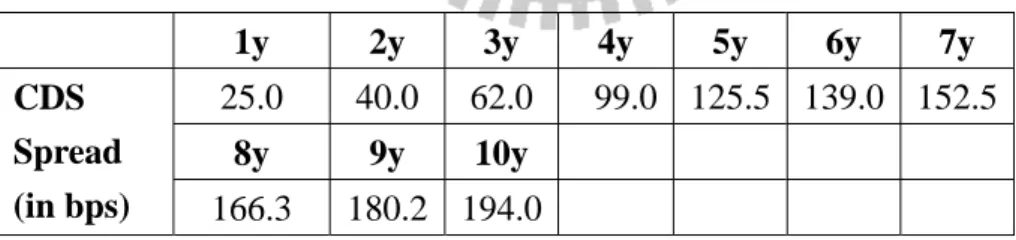
derive the default probabilities of different terms from the CDS spread of IBM quoted on 1/20/2006, compare those to the default probabilities calculated by Bloomberg, and plot the default probability curve. In the second example, in which the specified reference entity is the British Airway, we plot the current CDS spread curve and use input different jump rates to simulate the corresponding CDS spread curve 0.5 year after that date to see how the CDS spread term structure would shift when the underlying CDS spread has different jump rates. A reasonable guess is that the default probability curve as well as the CDS spread curve has a greater up ward movement as the jump rate increases. The input CDS spreads of British Airways is quoted on 4/11/2006 and the chosen parameters are: σ_kL = 0.25 and σ_kH = 0.35 for all k,

m_Y = 0.5, s= 0.2 . In both examples we use EURIBOR curve as the reference riskfree forward curve and set the recovery rate R be 0.4. Spreads data is listed in table 5.1.1. The results of example 1 and example 2 are respectively illustrated in figure 5.1.1 and figure 5.1.2.

Table 5.1.1: CDS spreads and default probabilities of IBM on 1/20/2006

Year Spread Model DP Bloomberg DP

0.5 6.576 0.0005 0.0005 1 6.576 0.0011 0.0011 2 10.230 0.0034 0.0035 3 13.915 0.0071 0.0071 4 16.748 0.0114 0.0115 5 19.581 0.0167 0.0169 7 27.608 0.0333 0.0339 10 39.642 0.0681 0.0707

QuickTime?and a TIFF (LZW) decompressor are needed to see this picture.

Figure 5.1.1 The default probability curve of IBM on 1/20/2006 derived

by this model and that calculated by Bloomberg.

Table 5.1.2 CDS mid spreads of British Airway (4/11/2006)

1y 2y 3y 4y 5y 6y 7y 25.0 40.0 62.0 99.0 125.5 139.0 152.5 8y 9y 10y CDS Spread (in bps) 166.3 180.2 194.0 QuickTime?and a TIFF (LZW) decompressor are needed to see this picture.

Figure 5.1.3 Widening of CDS spreads with different jump rates for the underlying CDS spread.

5.2 Implied Volatilities of Credit Default Swaptions

In this subsection we investigate the implied volatility structure of credit default swaption. Glasserman and Kou (2003) indicate the importance of jumps and stochastic volatility in implied volatility curve. Das and Sundarum (1999) investigate the shape of implied volatility in jump-diffusion and implied volatility models. We shall discuss how implied volatilities are related to jumps and discover how jump parameters of CDS spreads affect volatility structures of credit default swaption.

Consider the case of payer swaptions. Different implied volatility structures are demonstrated with respect to different inputs of jump parameters, which are jump rate, mean value of jump size and log-volatility of jump size of the corresponding CDS spread. The numerical experiment sets the jump intensity (or jump rate) of the underlying CDS spread to be λ_m,n =λ, the initial CDS spread to be 500 basis points, swaption time to maturity ( T ) to be two years with tenor-length (δ) six months.We also fix the riskfree forward rate (Lk) at 4% and assume a constant CDS spread volatility γ_m,n to be 0.25. The strike spread is ranged from 200 bps to 800 bps increasing by 50 bps. The following three different cases are considered.

In the first case we input different jump rates (λ) and hold other parameters fixed. The implied volatility tends to be higher as jump rate grows (see Table 5.2.1). Larger jump rate means the underlying CDS spread jumps more frequently, which in turn will push up swaption price as well as implied volatility.

Secondly, we allow the log-volatility of the jump size in CDS spread (s) to vary, with other parameters fixed, to examine how the implied volatility curve would fluctuate according to various inputs of s. The results are listed in Table 5.2.2. The climbing log-volatility of jump makes the implied volatility of CSO shift up. Since the more dispersed the underlying CDS spread is, the higher possibility big jumps would occur, which makes the CSO more hazardous and implied volatility larger.

In the last case, different values of mean jump size of CDS spread (mY) are input and other parameters are held fixed. Table 5.2.3 demonstrates the numerical results. It shows the various shapes of implied volatility curves with different mY. When the mean jump size is zero, it yields a volatility “smile”; while the nonzero mean jump size brings into a volatility “skew”, with an upward skew if mY > 0 and downward skew if mY < 0. The skew and smile phenomenon can be interpreted in terms of market’s expectation of jumps. In the case of positive mean jump size, an upward sloping volatility curve is the result of the possible large positive jumps which is concerned by the market participants. A downward skew volatility curve, where the mean jump size is negative, comes from the fear of large negative jumps. In the case

of m_Y = 0, the market has a symmetric anticipation for jumps, so the volatility curve is shaped as a smile. As is shown in Table 5.2.3 and Figure 5.2.3, the implied volatility curve of CSO whose underlying mean jump size equals to zero falls below that of CSO whose underlying mean jump size is greater or less than zero.

QuickTime?and a TIFF (LZW) decompressor are needed to see this picture.

Figure 5.2.1 Implied Volatility Curve of a credit default swaption with different jump

rates and fixed jump size mean and log-volatility, where mY = 0, s= 0.3

QuickTime?and a TIFF (LZW) decompressor are needed to see this picture.

Figure 5.2.2 Implied Volatility Curve of a two-year credit default swaption with different jump size log-volatility and fixed jump size mean and jump rate, where

λ = 0.5 , m_Y = 0.3.

QuickTime?and a TIFF (LZW) decompressor are needed to see this picture.

Figure 5.2.3 Implied Volatility Curve of a two-year credit default swaption

with different mean jump sizes and fixed jump rate and jump size log-volatility, where λ= 0.5 , = 0.25s

6. Conclusion

In this paper we assume that defaultfree and defaultable forward rates follow the jump diffusion process and model the jump parts with compound Poisson process. By this setting the credit spread and the hazard rate also have jump-diffusion dynamics. We then deduce a fair CDS spread formula from which default probabilities can be stripped. In the valuation of credit default swaption we treat the underlying CDS spread as the major variable and determine its jump-diffusive dynamics under the default swap measure. With this jump diffusion setting we are capable of fitting the distribution of CDS spread returns to the leptokurtic feature as can be seen in the market. The price of credit default swaption is attainable under a specific compound Poisson setting with its jump magnitude assumed to be lognormal. The pricing formula appears to be an infinite series, and it converges to Black-Scholes formula when the jump rate of the underlying CDS spread attends zero. A larger jump

rate will cause a higher swaption price. We also demonstrate how to derive the implied default probability from its CDS spread quote and show that the default probability curve has a greater upward movement as the jump rate is higher. Additionally, we exhibit the flexibility of our approach by illustrating the volatility “smiles” and “skews” from the swaption prices calculated by our pricing formula. Further empirical study is required in order to verify the effectiveness of this model. There are two more issues to be left for future studies: The first is to specify a more appropriate class of dynamics for the diffusion parts of the forward rates, and the mean-reversion process may be a good candidate; the second is to embed default correlations and extend this model to the pricing of multi-name credit derivatives such as CDOs.

References

Andersen, L., and J. Andreasen, 2000, “Volatility Skews and Extensions of the LIBOR Market Model”, Applied Mathematical Finance 7, 1-32.

Bennani, N., and D. Dahan 2004, “An Extended Market Model for Credit Derivatives”, Stochastic Finance 2004 Autumn School & International Conference.

Bjork, T., Y. Kabanov, and W.Runggaldier, 1997, “Bond Market Structure in the presence of Marked Point Processes”, Mathematical Finance 7, 211-239.

Brace, A., D. Gatarek, and M. Musiela, 1997, “The Market Model of Interest Rate Dynamics”, Mathematical Finance 7, 127-155.

Brigo, D., 2001, “Constant Maturity Credit Default Swap Pricing with Market Models”, Social Science Research Network.

Brigo, D., and L. Cousot, 2004, “A Comparison between the stochastic intensity SSRD Model and the Market Model for CDS Options Pricing”, The third Bachelier Conference, Chicago.

Brigo, D., and A. Alfonsi, 2005, “Credit Default Swaps Calibration and Option Pricing with the SSRD Stochastic Intensity and Interest-Rate Model”, Finance Stochastics IX (1).

Cont, R., and P. Tankov, 2004, Financial Modelling with Jump Processes (Chapman&Hall/CRC).

Das, S.R., and R. K. Sundarum, 1999, “The Surprise Element: Jumps in Interest Rate Diffusion”, Journal of Financial Quantitative Analysis 34, 211-240.

Glasserman, P., and N. Merener, 2003, “Cap and Swaption Approximations in LIBOR Market Models with Jumps”, Journal of Computational Finance 7, No. 1.

Glasserman, P., and S.G. Kou., 2003, “The Term Structure of Simple Forward Rates With Jump Risk”, Mathematical Finance 13, No. 13, 383-410. Hull, J., M. Predescu, and A. White, 2003, “The Relationship Between Credit

Default Swap Spreads, Bond Yields, And Credit Rating Announcement”. Jamshidian, F., 1997, “Libor and Swap Market Models and Measures”,

Finance Stochastics 1, 293–330.

Jamshidian, F., 2004, “Valuation of Credit Default Swaps and Swaptions”, Finance Stochastics 8, 343–371.

Jarrow, R.A., and S.M. Turnbull, “Pricing Derivatives on Financial Securities Subject to Credit Risk”, Journal of Finance L, 1, 53-85.

Merton R.C., 1976, “Option Pricing When Underlying Asset Returns Are Discontinuous”, Journal of Financial Economics 3.

Kou, S.G., 2002, “A Jump Diffusion Model for Option Pricing”, Management Science 48, 1086-1101.

Schönbucher, P.J., 2000, “A Libor Market Model with Default Risk”, Working Paper, Bonn University.

Shreve, S.E., 2004, Stochastic Calculus for Finance II: Continuous-Time Models (Springer).

Wu, L., 2005, “To Recover Or Not To Recover: That Is Not The Question”, Financial Mathematics Seminar at HKUST.

Zhou, C., 1997, “A Jump-Diffusion Approach to Modeling Credit Risk and Valuing Defaultable Securities”.

Appendix A – Change of measure with the inclusion of jumps

First we consider the case of marked-point-processes. For every defaultable bond price B(t) , the corresponding Radon-Nikodym derivative under default swap measure is Z(t )= dP m,n dP = B_m,n(t ) B(t ) B(0) B_m,n(0) = B(0) Bm,n(0) 1 1+δLj(Tj) 1 1+δLj(t ) j=η(t ) k

∏

k= m n

∑

j=0 η(t )

∏

The jump magnitude of _{Z (t)} is

Z(t)− Z(t−) = B(0) B_m,n(0)⋅ δ 1 1+δ L_j(t−)(1+ h_j( y,t)) j=η(t) k

∏

k= m n

∑

δ 1 1+δ L_j(t−) j=η(t) k

∏

k= m n

∑

= B(0) B_m,n(0)⋅ bk 1+δ L_j(t−) 1+δ L_j(t−)(1+ h_j( y,t)) j=η(t) k

∏

k= m n

∑

where b_k = Bk+1(t) δB_k+1(t) k= m n−1

∑

= B_k+1(t) B_m,n(t).

Let y denotes the jump magnitude of the defaultable forward rate, then _{Z (t)} can be written in a differential form:

dZ(t) Z(t−) = B(0) B_m,n(0){...dW (t)+ ( bk 1+δL_j(t) 1+δL_j(t)(1+ h_j( y,t)) j=η(t ) k

∏

k= m n

∑

°D

∫

− 1)(µ_P(dy, dt)− v_P(dy, dt))}

where from the jump-diffusion version of Girsanov theorem there exists a function Φ that satisfies the finite integrable condition such that

vPm ,n(dy,t)= Φ( y,t)vP(dy,t),

Specifically for compound Poisson processes here, h( y,t) will be replaced by _y, and the compensated measure _{v(dy, dt)} can be further specified by

v(dy, dt) =λf (dy)dt,

In consequence, we can write the desired function Φ( y,t) in a more specific form representing a direct relationship between the jump rates and densities of y in the original probability measure P and those in the default swap measurePm n, :

Φ( y,t) =λP m,n f_pm,n ( y) λPf_p( y) ( ) 1 ( ) 1 ( )(1 ) k n j k k m j t j L t b L t y η δ δ = = + = + +

∑ ∏

.

Appendix B – Derivation of the swaption price

C(t, S_m,n(t),T_m,T_n, S*, B_m,n(t)) = B_m,n(t)E_tm,n[C(T ,Tm,Tn, S*, Bm,n(T )) B_m,n(T ) ] = B_m,n(t)E_tm,n{[S_m,n(T )− S*]+} = B_m,n(t)E_tm,n{E_tm,n{[S_m,n(T )− S*]+|σ( N_T − N_t)} = B_m,n(t) E_tm,n{[S_m,n(T )− S*]+| N_T − N_t = j}⋅ P_m,n( N_T − N_t = j} j=0 ∞

∑

= B_m,n(t) e −λ_m,n(T−t) [λ_m,n(T − t)]j j! ⋅ E m,n {[S_m,n(T )− S*]+| N_T − N_t = j} j=0 ∞

∑

(*) By (4.7) we can replace Sm,n(T ) as S_m,n(T )= S_m,n(t)⋅ exp{ [−1 2γm,n(s) 2 ds+γ_m,n(s)dW_m,n(s) t T

∫

]−λ_m,nm_Y(T− t) + ln i=1 N_T− N_t

∑

(Y_im,n )}}

So the infinite series becomes

e−λm ,n(T−t ) [λ_m,n(T− t)]j j! ⋅ E m,n {[S_m,n(t)⋅ exp{ [−1 2γm,n(s) 2 ds+γ_m,n(s)dW_m,n(s) t T

∫

] j=0 ∞

∑

−λ_m,nm_Y(T − t) + ln i=1 j

∑

(Y_im,n)}− S*]+} = e −λ_{m ,n}(T−t ) [λ_m,n(T − t)]j j! ⋅ E m,n {[S_m,n(t)⋅ Y_im,n i=0 j

∏

⋅ exp{ [−1 2γm,n(s) 2 ds+γ_m,n(s)dW_m,n(s) t T

∫

] j=0 ∞

∑

−λ_m,nm_Y(T − t)}− S*]+}

We also know that

ln Sm,n(T ) is normally distributed with

E ln S_m,n(T )= ln S_m,n(t)− 1 2γm,n(s) 2 ds+λ_mnm_Y(T − t) t T

∫

[ln(1+ m_Y)−1 2s 2− 1] , and var(ln Sm,n(T ))= γm,n(s) 2 ds+λ_mn(T − t) t T

∫

s2

[S_m,n(t)⋅ e−λm,n(T−t )⋅ (1+ m Y) j⋅ N( ln[S_m,n(t)⋅(1+ m_Y)j]− ln(S*)+1 2( γm,n 2 (s)ds t T

∫

+ js2 ) γ_m,n2 (s)ds t T

∫

+ js2 ) −S*⋅ N( ln[S_m,n(t)⋅ (1+ m_Y)j]− ln(S*)− 1 2( γm,n 2 (s)ds t T

∫

+ js2 ) γ_m,n2 (s)ds t T

∫

+ js2 )]

As a result, the swaption price is

C(t, S_m,n(t),T_m,T_n, S*, B_m,n(t)) = e −λ_m,n(T−t ) [λ_m,n(T − t)]j j! BC(Sm,n ( j ) (t) j=0 ∞

∑

,T − t,S*,V_j2(t), B_m,n(t))