多品質特性製程的製程能力指標 CpkT 的分布和推論

國 立 交 通 大 學

統計學研究所

碩 士 論 文

Distributional and Inferential Properties of Capability

Index

C

T_pk

_{for Processes with Multiple Characteristics}

多品質特性製程的製程能力指標

T pk

C

的分布和推論

研 究 生 ：李美諭

指導教授 ：洪志真、彭文理 博士

中 華 民 國 九 十 八 年 六 月

Index

C

T_pk

_{for Processes with Multiple Characteristics}

多品質特性製程的製程能力指標

T

pk

C

的分布和推論

研 究 生：李美諭

Student：Mei-Yu Li

指導教授：洪志真

博士 Advisor：Dr. Jyh-Jen Horng Shiau

彭文理 博士 Dr. W. L. Pearn

國 立 交 通 大 學

統計學研究所

碩 士 論 文

A Thesis

Submitted to Institute of Statistics

National Chiao Tung University

in Partial Fulfillment of the Requirements

for the Degree of Master

in Statistics June 2009

Hsinchu, Taiwan, Republic of China

i

多品質特性製程的製程能力指標

T pk

C

的分布和推論

研究生：李美諭 指導教授：洪志真 博士

彭文理 博士

國立交通大學統計學研究所

摘要

與良率有關的製程能力指標 Cpk 在製造業中已經廣泛的被使用來評量製程之表現。 此方面多數的研究都著重在單一品質特性的製程，然而在實際的應用上，一個製程常常 是具有多個品質特性，而每個特性都有不同的規格。在這一篇論文中，我們研究將 Cpk 推廣為多個獨立的品質特性製程的 Cpk，因此新定義一個指標 CTpk。 我們證明了 T pk C 像 Cpk一樣與製程良率的上限跟下限有個一對一對應的關係。我們 也以理論證明的方式找出估計量 C 的常態近似分配，透過常態近似分配，統計假設Tpk 檢定、信賴區間、信賴下限都可以用來檢驗製程是否是有達到特定的標準。其中信賴下 限在實務上特別重要，因為信賴下限可以用來估計製程的最小能力，與品質保證有很大 的相關性；而精確性 (R) 則是估計量與信賴下限的比值，定義這個值是為了方便工程 師每天量測製程的最小能力。接著透過資料模擬的方式，檢驗常態近似分配逼近估計量 真正分配的準確性。

最後，我們用一個實際的製程－雙蕊光纖(a dual-fiber tip process) 作為例子，說明 如何將新提出的指標及本文所提出之統計推論方法應用到實際的製程上。

ii

Distributional and Inferential Properties of Capability

Index

C

T_pk

_{for Processes with Multiple Characteristics}

Student:

Mei Yu Li

Advisor:

Dr. Jyh-Jen Horng Shiau Dr. W. L. Pearn

Institute of Statistics,

Department of Industrial Engineering & Management,

National Chiao Tung University, Taiwan

Abstract

Process capability index Cpk has been popularly used in the manufacturing industry for

measuring process performance based on yield (proportion of conformities). Most researches on Cpk focus on processes with single quality characteristic; but in many real applications, a

process often has multiple quality characteristics. In this study, we extend Cpk to a new index

T pk

C for processes with multiple characteristics. We prove that the inequalities that link Cpk to

the yield also hold for the new index. A natural estimator of CTpk is provided and a normal

approximation to its distribution is derived. With this normal approximation, standard processes for statistical inferences such as hypothesis testing and confidence interval are developed for testing whether the process is capable and providing an interval estimate on

T pk

C , respectively. More importantly, we can obtain a confidence lower bound for CT_pk, which measures the minimum process capability and is directly linked to quality assurance of products. The accuracy of the normal approximation is studied by simulation. Finally, we demonstrate how the new index CT_pk as well as the inferential procedures developed in this

iii

iv

致 謝

兩年的碩士生涯即將邁向終點，很快的即將踏入人生的另一個旅程。回首當初在交 大統計所的榜單上查到自己是正取時，那種既興奮又期待的心情，以及現在豐收的喜 悅，「不虛此行」的感觸油然而生。謝謝這兩年來，對於我的懵懂給予提攜以及在我無 助時，對我伸出援手的所有人。 首先要感謝我的指導教授－彭文理老師。雖然，跟著老師做論文，挑戰性很大，遇 到問題時要自己想辦法、找資源；出現瓶頸時，要靠自己去突破。老師只在每個階段的 里程碑等著我，告訴我下個階段要達成的目標是什麼。這樣的過程，雖然很艱辛，但卻 也讓我真的學會做論文。在寫論文時，老師也秉持著高標準來要求我，但卻也是這樣的 要求激發了我嘗試想突破障礙、努力達到老師要求的潛能。因此，跟著老師做研究的這 一年，讓我覺得生活過得既充實又有成就感。 再來，要感謝我的另一位指導老師－洪志真老師。感謝老師在我做論文遇到障礙 時，給予我方向；碩士論文高標準的寫作要求，讓我學習到一篇論文要完成，並不是隨 隨便便寫一寫就可以了，必須一而再，再而三的修改，讓我對論文編輯有了更上一層的 進步。 除此之外，特別要感謝洪慧念老師，在我升碩二的暑假適逢洪志真老師出國的這 段期間，每當我論文遇到瓶頸或是結果需要理論證明支持時，給予我很大的協助跟指導。 謝謝我的口試委員教授，在百忙之中為我口試，在口試時對於我的指導，更讓我 發現本論文主題可以更深入探討的地方，這在我的工作領域上有很大的幫助，能夠真正 達到學以致用的目標。 除此要特別感謝我們所上的助理郭碧芬小姐，她 總是不辭勞苦幫我們處理很多行 政事務上的問題，以及很好心的擔任當彭老師找我時的接線生，真的很感謝郭姐。 最後要感謝我的家人給我的支持，與家人相處的時間很少，因為爸媽的體 諒，才能 專心完成學業。 另外還有很多曾經幫助過我的朋友，因為有大家的幫助，才能有今天的成果。 2009 年 6 月 李美諭

v

Contents

Chapter 1. Introduction

1

Chapter 2.

Capability measure for multiple characteristics

3

Processes with multiple independent characteristics………..4

Chapter 3.

A new process yield index for multiple independent characteristics

4 3.1. The yield-related indexCT_pk……… . . . 4

Chapter 4. Estimation of

C

T_pk

5

4.1. The approximate distribution for a natural estimator of CT_pk………….………5

4.2. Statistical inferences based on the normal approximation………...7

Chapter 5. Accuracy of the Normal Approximation

9

5.1. A precision measure of CT LB_pk ………....…...9

5.2. Bias of the natural estimator of CT_pk……….……10

5.3. Simple size for required margin of error………...11

Chapter 6. An application example

11

Chapter 7. Conclusions

12

References

……….14

Appendix A

………...16

vi

Appendix C

………...19

vii

List of Figures

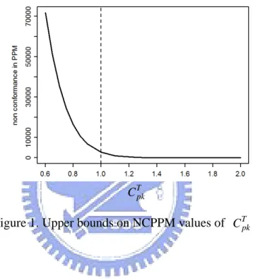
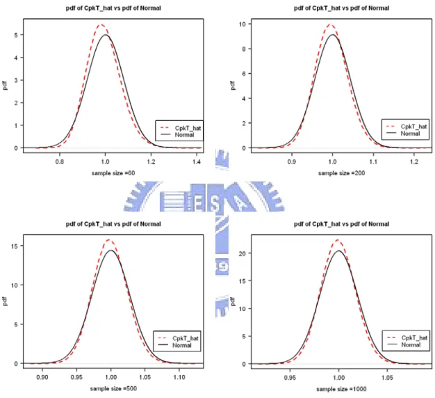
Figure 1. Upper bounds on NCPPM values of CT_pk……….………..20 Figure 2. Comparison of the probability density function (dash line) of CTpk obtained by

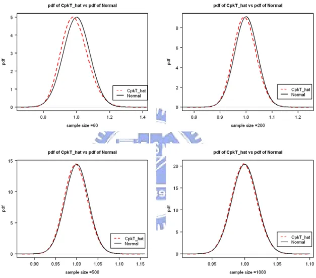
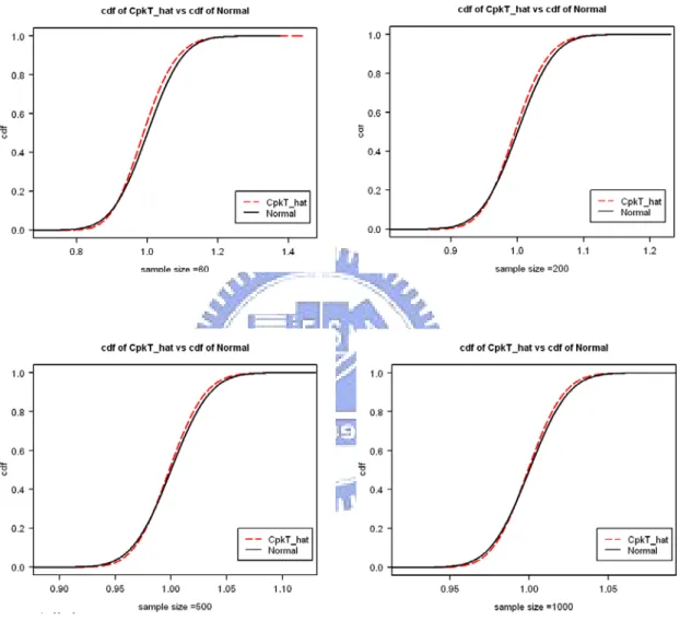
simulation and its normal approximation (solid line) for n = 60, 200, 500, 1000 (CT_pk =1.0 and µ₁≠m₁ and µ₂ ≠m₂)………...21 Figure3. Comparison of the distribution function (dash line) of CTpk obtained by simulation

and its normal approximation (solid line) for n = 60, 200, 500, 1000 (CT_pk =1.0 and

1 1 and 2 2

µ ≠m µ ≠m )………...22 Figure 4. Comparison of the probability density function (dash line) of CTpk obtained by

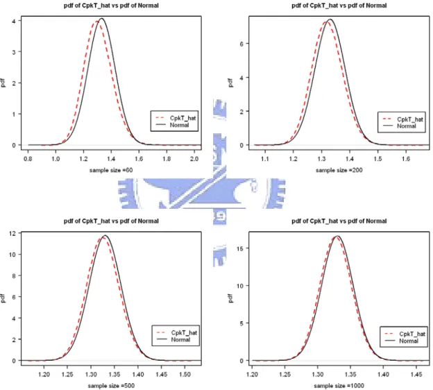
simulation and its normal approximation (solid line) for n = 60, 200, 500, 1000 (CT_pk =1.33 and µ₁=m₁ and µ₂ =m )………...23 ₂ Figure 5. Comparison of the distribution function (dash line) of CTpk obtained by simulation

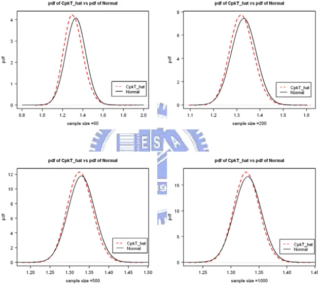
and its normal approximation (solid line) for n = 60, 200, 500, 1000 (CT_pk = 1.33 and µ₁=m₁ and µ₂ =m )………...24 ₂ Figure 6. Comparison of the probability density function (dash line) of CTpk obtained by

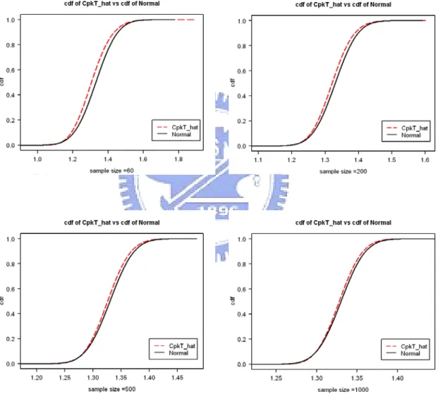
simulation and its normal approximation (solid line) for n=60, 200, 500, 1000 (CT_pk = 1.33 and µ₁ ≠m₁ and µ₂ ≠m )………...25 ₂ Figure 7. Comparison of the distribution function (dash line) of CTpk obtained by simulation

and its normal approximation (solid line) for n = 60, 200, 500, 1000 (CT_pk =1.33 and µ₁≠m₁ and µ₂ ≠m )………...26 ₂ Figure 8. Comparison of the probability density function (dash line) of CTpk obtained by

simulation and its normal approximation (solid line) for n = 60, 200, 500, 1000 (CT_pk =1.33 and µ₁=m₁ and µ₂ =m )………...27 ₂ Figure 9. Comparison of the distribution function (dash line) of CTpk obtained by simulation

and its normal approximation (solid line) for n = 60, 200, 500, 1000 (CT_pk = 1.33 and µ₁=m₁ and µ₂ =m )………...28 ₂ Figure 10. Curves of T LB

pk

C versus (Cpk1, Cpk2) with α = 0.05 and n =10(20)90 (from bottom

to top in plot)……….………..29 Figure 11. Curves of T LB

pk

C versus Cpk1 for variousCTpk, α = 0.05, and n = 10(20)90 (from

bottom to top in plot)……….………..30 Figure 12. A sample of the dual-fiber tips. from Pearn and Wu (2005b).………..31

viii

List of Tables

Table 1. Corresponding upper bounds of NCPPM for some specific values of CT_pk……….31 Table 2. Coverage rate and 90% confidence interval length (in parentheses) for various cases

of CT_pk=1.0 with n =30, 50, 100, 500, 1000..………...32 Table 3. Coverage rate and 90% confidence interval length (in parentheses) for various cases

of CT_pk=1.33 with n =30, 50, 100, 500, 1000..………...33

Table 4. Coverage rate and 90% confidence interval length (in parentheses) for various cases of CT_pk=1.5 with n =30, 50, 100, 500, 1000..……….34 Table 5. Coverage rate and 90% confidence interval length (in parentheses) for various cases

of CT_pk=2.0 _{with n =30, 50, 100, 500, 1000..……….35}

Table 6. The most conservative 95% lower confidence boundsCT LB_pk of CT_pk for CTpk

=1(0.1)2, n=10(10)200………..………..36 Table 7. The largest possible 95% lower confidence bounds CT LB_pk of CT_pk for CTpk=

1(0.1)2, n =10(10)200………..………37 Table 8. The precision R for the most conservative 95% lower confidence bounds CT LB_pk of

T pk

C for CTpk=1(0.1)2, n =10(10)200……….38

Table 9. Estimates of E(CTpk)and their standard errors (in parentheses) for some cases of 1.0

=

T pk

C and various n………..………..39 Table 10. Estimates of E(CTpk)and their standard errors (in parentheses) for some cases

=1.33

T pk

C and various n………..40

Table 11. Estimates of E(CTpk)and their standard errors (in parentheses) for some cases of

1.5 T pk

C = and various n……….41 Table 12. Estimates of E(CTpk)and their standard errors (in parentheses) for some cases of

2.0 T pk

C = and various n……….……42 Table 13. Sample sizes required for a specified margin of sampling error……….…….43 Table 14. Sample mean, sample standard deviation, specifications of individual characteristics

for the dual-fiber tips, and the estimated capability indices………..….…….44

1

1. Introduction

Process capability indices (PCIs) are often used as a quality measure to evaluate the performance of a process. Because PCIs establish the relationship between the actual process and the manufacturing specifications, they have been widely used in the manufacturing industries in recent years. Basic capability indices, Cp, CPU, CPL, Cpk, Cpm, Cpmk , are developed

for measuring whether a process has the reproduction capability (Kane (1986), Chan et al. (1988), Pearn et al. (1992), Kotz and Lovelace (1998), and Kotz and Johnson (2002)). Boyles (1991, 1994) proposed another index called Spk. These indices are defined as:

= 6 p USL LSL C σ − , = 3 PU USL C µ σ − , = 3 PL LSL C µ σ − , = min , 3 3 pk USL LSL C µ µ σ σ − −      , 2 2 6 ( ) pm USL LSL C T σ µ − = + − , = min 2 2 , 2 2 3 ( ) 3 ( ) pmk USL LSL C T T µ µ σ µ σ µ  _{− −}      + − + −     , 1 1 1 1 = ( ) ( ) 3 2 2 pk USL LSL S µ µ σ σ −  − −  Φ _ Φ + Φ _  ,

where USL and LSL are the upper and the lower specification limits, respectively, µis the process mean, σ is the process standard deviation, and T is the target value. While the indices Cp, Cpk, Cpm, Cpmk, and Spk are appropriate for statistically in-control normal processes with

two-sided specification limits, the indices CPU _{and C}PL _{are designed specifically for processes}

with one-sided specification limit.

The first known index Cp measures only the distribution spread, which only reflects

product quality consistency (in terms of process precision) but does not account for the location of process meanµ. The index Cpk not only takes into account the process variation

and the extent of process centering, but also measures actual process performance based on yield (i.e., proportion of conformities). If the value of Cpk is given for a process, Boyles (1991)

gave an upper bound and a lower bound for the process yield (denoted by %Yield) as 2Φ(3Cpk)－1≤% Yield ≤Φ(3Cpk), (1.1)

where Φ() is the cumulative distribution function (c.d.f.) of the standard normal distribution. For instance, if Cpk = 1.33, then the lower bound guarantees that the yield will be no less than

2

non-conformities. The inequalities in (1.1) link the index Cpk with the process yield. The last

index Spk provides an exact measure of the process yield, because the index is defined as a

monotonically increasing function of the yield. For example, if Spk= 1.33, then the exact yield

is 99.9933927%, or equivalently, 66.073 PPM of non-conformities.

The capability measuring for processes with single characteristic has been investigated extensively, but is comparatively neglected for processes involving multiple characteristics. However, it is quite common that industrial processes nowadays have more than one quality characteristic. Thus, the performance evaluation of multivariate processes has become more and more important.

Each of the multiple characteristics must meet certain specifications. However, the assessed quality of a product depends on the combined effects of the multiple characteristics, rather than on their individual values.For instance,a process manufacturing dual-fiber tips, a component is used to make fiber optic cables, has six quality characteristics, namely, the capillary diameter, length, wedge, core diameter, return loss, and polishing direction. These characteristics are related through the composition of the fiber tips. Therefore, it is natural to consider a multivariate characterization of this process.

The purpose of this study is to define a multivariate PCI, called CT_pk, for multivariate processes, which is a natural extension of the index Cpk for univariate processes; and most

importantly, the new index still retain the link to the yield as given in the expression (1.1). A natural estimator CTpk _for CT_pk is provided. Since the distribution of 

T pk

C _is

mathematically intractable, we derive its asymptotic distribution and obtain a normal approximation accordingly. For quality assurance, a lower bound of the yield is a valuable quality measure. We use this normal approximation to obtain a confidence lower bound of

T pk

C from process data.

The contents of this thesis is divided into seven sections. In Section 2, we emphasize the importance of studying multivariate process capability indices and review recent studies on the performance evaluation of multivariate processes. In Section 3, we propose a new yield index CT_pk for the overall process and relate it to the corresponding non-conformities in parts per million (NCPPM). In Section 4, we derive the asymptotic distribution of a natural

3

estimator CTpk of CT_pk and use this result to provide a confidence interval and a lower

confidence bound of the new index for processes with multiple independent characteristics. To investigate how well the approximation is to the actual distribution, we compare the normal approximation with the actual distribution of CTpk by simulation. Moreover, the

coverage rate and the confidence interval length are computed and the behavior of the lower confidence bound is investigated. In Section 5, we compute the most conservative lower confidence bound and the precision of the natural estimator for specified sample sizes, and investigate the accuracy of the normal approximation by simulation. A simulation study is conducted to investigate the bias of the natural estimator. In Section 6, as an illustrative example, we apply the methodology to a set of real data presented in Pearn and Wu (2005b). In Section 7, we conclude the thesis with a brief summary.

2. Capability Measures for Multiple Characteristics

In recent years, more and more researchers have been devoted to studying multivariate capability indices. For example, Chen (1994), Boyles (1996) and others presented multivariate capability indices for assessing capability. Wang and Chen (1998-1999) and Wang and Du (2000) proposed multivariate equivalents for Cp, Cpk, Cpm, and Cpmk based on

the principal component analysis, which transforms the original correlated variables into a set of uncorrected variables that are linear combinations of the original variables. Moreover, a comparison of three recently proposed multivariate methodologies for assessing capability are illustrated and discussed in Wang et al. (2000). On the other hand, some researchers modified the univariate index for processes with multiple characteristics. For example, Chen and Pearn (2003) modified the process capability index Spk to

(

)

1 1 1 2 (3 ) 1 1 / 2 3 i m T pk pk i S − S =      = Φ _ Φ − + _{ }    

∏

,

where Spki is the Spk of the ith characteristic. Later, Pearn and Wu (2005a) proposed the

following modified one-sided index, which is a generalization of the one-sided index CPU,

1 1 1 = (3 ) 3 i m T PU PU i C − C =     Φ _ Φ _   

∏

,

4

Processes with multiple independent characteristics

When a processes has m ( >1) independent characteristics, Bothe (1992) considered m yield measures P1,…,Pm and suggested the overall process yield P to be measured by P =

min{P1,…,Pm}. We can see that this approach does not reflect the real situation accurately.

Assuming the process has five characteristics (m = 5) with equal yield measures P1= P2 = P3

= P4 = P5 = 99.9934%. Using Bothe’s approach, the overall process yield is evaluated as P =

min{P1,…,Pm}=99.9934% (or 66 PPM of non-conformities). Supposing that the five

characteristics are mutually independent, then the overall process yield should be calculated as P1 × P2 × P3 × P4 × P5 = 99.967% (or 330 PPM of non-conformities), which is significantly

less than that suggested by Bothe (1992). (See Pearn and Wu (2005b) ).

In the manufacturing industry, Cpk has been popularly used for measuring process

performance because it can link to the process yield. In this paper, we define a new yield-related process capability index for processes of multiple independent characteristics. We consider a normal approximation to the distribution of the natural estimator to find the lower confidence bound, which gives us not only a clue on minimum actual performance related to the fraction of non-conforming units, but also is useful in decision making on the capability test.

3. A New Process Yield index for Multiple Independent Characteristics

3.1. The yield-related index

C

T_pk

For a process with m quality characteristics, we assume the m characteristics follow mutually independent normal distribution, 2

( _i, _i ), 1,..., .

N µ σ i= m Denote the two-sided specification limits of the ith characteristic by USLi and LSLi, i=1,…,m.

Given a value of Cpki, by (1.1), the individual yield of the ith characteristic has the following

bounds

2 (3Φ C_pki) 1 % − ≤ Yield_i ≤ Φ(3C_pki), i=1,..., . (3.1)m

If we wish to extend the notion of Cpk to a multivariate yield capability index CT_pk, it is

natural to require T pk

5

2 (3Φ CT_pk) 1 %− ≤ Yield≤ Φ(3CT_pk), (3.2)

where %Yield is the overall process yield of the multivariate process. Since the characteristics are mutually independent, by (3.1),

(

)

1 2 (3 ) 1 = Φ −

∏

m pki i

C is a lower bound of the overall process yield. Thus, if we set

(

)

1 2 (3 ) 1 2 (3 ) 1, (3.3) = Φ − = Φ −

∏

m T pki pk i C C then the first inequality in (3.2) automatically holds. Therefore, by equation (3.3), it is natural

to propose a new index as defined by

(

)

1 1 1 2 (3 ) 1 1 / 2 . (3.4) 3 − =    = Φ _ Φ − + _{ }   

∏

i  m T pk pk i C C

It can be shown that the inequality % (3Yield ≤ Φ CT_pk) holds as well. Derivation is given in Appendix A. Therefore, the new index defined as (3.4) satisfies (3.2). The new index

T pk

C may be viewed as a generalization of the single characteristic yield index Cpk and it

provides a lower bound of the overall process yield. Therefore, the corresponding upper bound (UB) of non-conformities in parts per million, NCPPM, for a well-controlled process with multiple independent normal characteristics can be calculated as

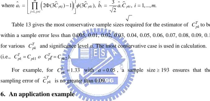
NCPPM ≤106×2[1− Φ(3CT_pk)]. (3.5) Table 1 and Figure 1 present the corresponding upper bounds of NCPPM for CT_pk= 1.00, 1.25, 1.33, 1.45, 1.50, 1.60, 1.67, and 2.00.

4. Estimation of

C

T_pk

4.1. The approximate distribution for a natural estimator of

C

T_pk

Let X ,₁ , X_nbe independent and identically distributional (i.i.d.) as a multivariate normal process N_m

(

µ,Σ

)

, where X_j =(X ,_1j , X ) , _mj ′ µ =(µ₁,,µ_m) , and is the ′ 　Σ m m×

diagonal matrix with diagonal elements 2 2 1,..., m.

σ σ

Since the individually Cpk can be expressed as

| | , 1,..., , 3 i i i pki i d m C µ i m σ − − = =

where µ_i is the mean of the ith characteristic, m_i = (USL_i +LSL_i) / 2is the mid-point of the specification interval, and d_i = (USL_i −LSL_i) / 2 _{is the half width of the specification interval.}

6

It is common to estimate Cpki by

 | X | , 3 − − = _i i _i pki i d m C S (4.1) 2 2 1 1 1 1 where X = X and S = (X X ) , = 1,..., . 1 = = − −

∑

n

∑

n i _{ij i ij} i j j i m n n (4.2)

To estimate the index CT_pk, we consider the following natural estimator

 1

(



)

1 1 = 2 (3 ) 1 1 / 2 , 3 m T pk pki i C − C =      Φ _ Φ − + _{ }    

∏

 (4.3) where Cpki is the Cpk of the ith characteristic.

.

Theorem 1.

The exact distribution of CTpk _{is analytically extractable; however, it can be shown that} T

pk

C _{has an asymptotic normal distribution as stated in the following theorem. The}

asymptotic distribution of CTpk _is

(



)

₂ 2 2 1 1 0 , ( ) as , (4.4) 9 φ(3 ) =     − → + → ∞  _{ }    

∑

 m d T T pk _{pk i i} T i pk n C C N a b n C where

(

)

1, 3 = 2 (3 ) 1 (3 ) and = , = 1,..., . 2 m i pkj pki i i pki j j i a C φ C b a C i m = ≠   Φ −   

∏



We give two different proofs in Appendix B and Appendix C, respectively.

Note that, by equation (4.4), CTpk _{is asymptotically unbiased. To see how well the}

normal approximation is, we conduct a simulation study using the free statistical package R as follows. Four scenarios are considered in the simulation study, the combinations of two CT_pk

values (1 or 1.33) and two cases of process mean (µ_i ≠m_i or µ_i =m_i, i=1, 2). For each scenario, simulate 1,000,000 random samples of size n = 60, 200, 500, 1000 from

2 2

2( 1, 2, 1 , 2 , 0)

N µ µ σ σ , a normal process with two independent characteristics. For each scenario, we compute 1,000,000 CTpk by (4.3). Figures 2-9 compare the simulated

distribution obtained by 1,000,000 CTpk′s to the normal approximation with their probability

7

sample size n reaches 1000, the approximate and simulated distributions are very close. In fact, even with n = 60, the approximation is already quite reasonable for practical purposes.

4.2 Statistical inferences based on the normal approximation

With the asymptotic distribution given in equation (4.4), we now can make statistical inferences on CT_pk based on a set of random samples, including the hypothesis testing, confidence interval, and lower confidence bound.

To test whether a given process is capable, we consider the following statistical hypothesis testing:

0

1

H : (the process is not capable) H : (the process is capable)

≤ > T pk T pk C c C c (4.5)

where c is the minimal standard criterion on CT_pk.

The test can be executed by considering the testing statistic

  2 2 1 3 (3 ) , φ =  ₋      =  ₊     

∑

 T T pk pk m i i i n C c C T a b _(4.6) 

(



)

   1, 3 where = 2 (3 ) 1 (3 ) and = , = 1,..., . 2 φ = ≠   Φ −   

∏

  m i pkj pki i i pki j j i a C C b a C i m

Because we do not know the values of a₁, a₂, , and ,b₁ b we estimate them from data. ₂ The null hypothesis Ho is rejected at α level if T > Zα, where Zα is the upper 100α% percentile

of the standard normal distribution.

An approximate 100(1- α)% confidence interval for CT_pk can be easily obtained as

      1/ 2 1/ 2 2 2 2 2 2 ₁ 2 ₁ 1 1 ( ) , + ( ) (4.7) 9 [ (3 )] 9 [ (3 )] α α φ = φ =  _{   }       _{−  +   + }   _{   }       

∑

m 

∑

m  T T pk _T i i pk _T i i i i pk pk C Z a b C Z a b n C n C

and an approximate 100(1- α)% lower confidence bound for CT_pk can be expressed as

8    1/ 2 2 2 2 1 1 ( ) , (4.8) 9 [ (3 )] α φ =     ≈ − +   

∑

  m T T LB pk i i pk T i pk C C Z a b n C 　　　 

where and are as before.ai bi

To evaluate the proposed confidence interval and lower bound of CT_pk, we conduct a simulation study. We use equation (4.7) to obtain confidence interval and confidence interval length. Consider the case of CT_pk=1.33 with 90% confidence level under a process of two independent characteristics. Note that there are infinite number of the combinations of the process distribution and the manufacturing specifications that would correspond to the same value of CT_pk=1.33. We consider six scenarios as given in Table 3 in the study.

For each scenario, generate N=1,000,000 random samples of size n =30, 50, 100, 500, 1000 from N u₂( , ₁ u₂,σ₁2, σ₂2, 0 ). For each case, we compute 1,000,000 CTpk , the

corresponding 1,000,000 confidence intervals and CT LB_pk ′ . Check if the true index s CT_pk is contained in the interval and if it is greater than CT LB_pk .

Tables 2-5 present the coverage rate and the average length of 1,000,000 confidence intervals. We can find that the coverage rate approaches 0.9 (under α = 0.1) and the confidence interval length is decreasing to zero as the sample size n increases.

For the univariate case, Pearn and Shu (2003) examined the behavior of the lower confidence bound of Cpk against ξ , where ξ =

(

µ− m

)

/σ. Since for a process with two

characteristics, CT LB_pk involves ξ_{1 and} ξ₂ . However, there are too many Cpki’s

corresponding to one ξ_i. Therefore, instead, we explore the relationship between CT LB_pk and (Cpk1, Cpk2). To do this, instead of performing simulation experiments that require extensive

calculations, we calculate and plot

1/2 2 2 2 1 1 ( ) (4.9) 9 [ (3 )] α _φ =   ≈ −  +    

∑

 m T LB T pk pk _T i i i pk C C Z a b n C

versus Cpk1 and Cpk2 to examine the relationship between CT LB_pk and (Cpk1, Cpk2 ).

Based on CT LB_pk expressed in equation (4.9), given sample size n = 10, 30, 50, 70, 90, Figure 10 displays the curves of CT LB_pk versus various combinations of Cpk1 and Cpk2 with

T pk

9

10, 30, 50, 70, 90 for T pk

C = 1.0, 1.33, 1.5, 1.67. We examine the results of calculation and find that

 T LB

pk

C reaches its absolute maximum when Cpk1 = Cpk2.

 The minimum of CT LB_pk occurs when one of C_pk′s approaches infinity, that is, when CT_pk equals one of C_pk′s. This minimum is the most conservative lower confidence bound for a given CT_pk.

From Figure 10 and Figure 11, we can also observe the above properties.

5. Accuracy of the Normal Approximation

For a given CT_pk, by setting one Cpk at CTpk and the other Cpk at ∞ , we can use

equation (4.9) to compute the most conservative CT LB_pk , which represents a measure of the minimum manufacturing capability of the process for the case when the process has two independent characteristics. For engineer convenience, if a process with two independent characteristics has CTpk =1.33and sample size n =100, then we have 95% confidence to say

that the true CT_pk of this process is no less than 1.1392. Similarly, we can compute the largest possible CT LB_pk by setting Cpk1 = Cpk2. The largest possible value of CT LBpk may not have

much of the practical value, but is of interest mathematically.

Tables 6 and 7 tabulate both the most conservative and largest possible CT LB_pk value for

T _1(0.1)2

pk

C = , n=10(10)200 and confidence level γ = 95%.

5.1. Accuracy analysis of

C

T LB_pk

Sample size determination is important, as it directly relates to the cost of the data collection. By equation (4.8), we have

    2 2 2 2 1 2 ( ) ( / ) 1 / . (4.10) 9[ (3 )] α φ − =   +       ≈ _{  } − _    

∑

m _i _i T _{i T LB} T pk _{T pk} pk pk a b n Z C C C C 

(



)

   1, 3 where = 2 (3 ) 1 (3 ), = , = 1,..., . 2 m i pkj pki i i pki j j i a C φ C b a C i m = ≠   Φ −   

∏

 

10

To evaluate the precision of the lower confidence bound CL_pmfor the index Cpm given

earlier, Pearn and Shu (2003) defined a precision measure R=C_pmL /Cpm, where Cpm is a

natural estimator of Cpm. Similarly, for CT LBpk we can define / 

T T LB

pk pk

R=C C . In Table 8, we tabulate the value R of the most conservative CT LB_pk for processes with two independent characteristics. These values can be useful for engineers and practitioners, because it would be convenient to assess the minimum capability of the process for engineers as a everyday work.

For example, if one requires a 95% lower confidence bound for CT_pk to be of 85% precision of CTpk _(i.e., / 0.85

T T LB

pk pk

C C = ) for CTpk =1.5, then the most conservative sample

size required for achieving this goal is 66, which can be computed by

    2 _{2 2} 2 2 1 2 ( ) ( / ) 1 / . 9[ (3 )] α φ − =   +       ≈ _ − _        

∑

_i _i T _{i T LB} T pk _{T pk} pk pk a b n Z C C C C ₁  _{2 1} 3   ₂ where (3 ), 0, = (3 ) , and = 0. 2 φ φ = Tpk =  Tpk Tpk  a C a b C C b

On the other hand, if one obtains a CTpk =1.5from a set of data of size 66, then the most

conservative 95% lower bound can be conveniently obtained by multiplying CTpk by the

corresponding R (=0.85), i.e., the most conservative lower bound is 1.5 0.85 1.275× = . One then can conclude that the true value of the process capability CT_pk is no less than 1.275 with 95% confidence.

5.2. Bias of the natural estimator of

C

T_pk

In order toexplore the bias of the natural estimator by simulation, we simulate a total of N=1,000,000 replications for each sample size of n = 30, 50, 100, 500, 1000. Take the average of N CTpk′s to estimate ( )

T pk

E C _{and compare it with the true} CT_pk. The simulation results presented in Tables 9-12indicate that the bias is negative for the cases under study. That is, we underestimate CT_pk when the yields of the two independent characteristics are the same (i.e., Cpk1 = Cpk2). On the other hand, when one %Yield almost reaches 100% (i.e., when

1 2

= =

T T

pk pk pk pk

C C o C r C ), the problem is basically reduced to the univariate case, a situation previously studied by Kotz et al. (1993). They showed that the natural estimator Cpk _{of C}pk

11

is biased and the bias is positive whenµ≠m _{( µ is the process mean and}mis the midpoint of the specifications). Whenµ=m, the bias is positive for sample size≤10, but is negative for larger values of sample size. See Kotz et al. (1993) for more details.

5.3. Sample size for required margin of error

From (4.8), the margin of sampling error is approximately note that

  1/ 2 2 2 1 2 ( ) . 9 [ (3 )] m i i i T pk a b Z n C α φ =  _{∑ +}           

(



)

   1, 3 where = 2 (3 ) 1 (3 ), = , = 1,..., . 2 φ = ≠   Φ −   

∏

  m i pkj pki i i pki j j i a C C b a C i m

Table 13 gives the most conservative sample sizes required for the estimator of CT_pkto be within a sample error less than 0.005, 0.01, 0.02, 0.03, 0.04, 0.05, 0.06, 0.07, 0.08, 0.09, 0.1 for various CT_pk and significance level α. The most conservative case is used in calculation. (i.e., CT_pk =C_pk1 o CT_pkr=C_pk2).

For example, for CT_pk =1.33 with α= 0.05, a sample size≥193 ensures that the sampling error of CTpk _{is no greater than 0.09.}

6. An application example

For illustration, we consider a real example presented in Pearn and Wu (2005b), which is taken from an optical communication manufacturing factory located in Science-based Industrial Park in Taiwan. The example involves a process manufacturing dual-fiber tips, a component used in making fiber optic cables.

Figure 12 depicts a sample of the dual-fiber tips. Sixty dual-fiber tips were taken from a

stable (i.e., in statistical control) process in the factory, and two product quality characteristics were measured, (i) Capillary length and (ii) Wedge. For a particular model of dual-fiber tips, the specifications of characteristics are listed in Table 14. According to Pearn and Wu (2005b), it is reasonable to assume that these 60 data were from a normal distribution with two independent quality characteristics. The sample mean, standard deviation, and specifications along with the individual Cpk of each characteristic are summarized in Table 14.

12

If the quality requirement was predefined as CT_pk ≥1.33, then we can make some statistical inferences on CT_pk by using hypothesis testing and interval estimation. For testing the null hypothesis Ho as given in (4.5) with c =1.33, the testing statistic T given in (4.6) is

2.321008 > Z0.05 = 1.645. Thus, Ho is rejected at α = 0.05. We conclude that the process meets

the capability requirement of CT_pk >1.33 with 95% confidence.

Moreover, C = 1.702917Tpk _and CT LBpk =1.438560by (4.3) and (4.8), respectively. Thus,

we have 95% confidence to say CT_pk is no less than 1.43856, or equivalently, there are no more than 16 PPM of non-conformities as given in (3.5).

7. Conclusions

Process yield is the most common criterion used in the manufacturing industry for measuring process performance. The widely used capability index Cpk is a yield-related index,

in the sense that it can provide a lower bound for the yield of a process with single characteristic. But in many real applications, the process has multiple characteristics.

In this paper, we extend Cpk to an index CTpk to assess the yield of processes with

multiple characteristics. It is shown that 2 (3Φ CT_pk) 1 % (3− ≤ Yield≤ Φ CT_pk), a property holds for the univariate Cpk. Based on the new index CTpk, the practitioners can make reliable

decisions for capability testing and monitoring the overall performance of all process characteristics.

Unfortunately, the distributional properties of the natural estimator CTpk are

mathematically intractable. We derive a normal approximation to the distribution of the CTpk

by the first-order Taylor expansion and investigate the accuracy and precision of CTpk by

simulation.

Applying the asymptotic distribution of CTpk, hypothesis testing, confidence interval,

and a confidence lower bound CT LB_pk are constructed. We investigate the behavior of CT LB_pk versus Cpk1 and Cpk2 for given CTpk′s and find that the most conservative lower bound can

be obtained by setting one of C_pk′s at the given CT_pk and the other at infinity. We also provide tables for engineers or practitioners to use in assessing their processes. On the other hand, it is also found that CT LB_pk reaches its absolute maximum when Cpk1 = Cpk2.

13

As an illustrative example, an application example on dual-fiber tips taken from Pearn and Wu (2005b) is employed. The practical implementation of the statistical theory for manufacturing capability assessment bridges the gap between the theoretical development and the in-plant applications.

For the future research, we could consider the following topics:

 Use the second-order expansion of Taylor series to approximate the distribution of

T pk

C _{to get a more accurate approximation.}

 Generalize T pk

C for processes with asymmetric tolerances.  Explore the similar research to T

pk

C for Cp, CPU, CPL, Cpk, Cpm, Cpmk.

 Develop appropriate process capability measurement based on T pk

C when gauge measurement errors exist.

Followings are some other potential research topics:

 develop a powerful test for on-sided or two-sided supplier selection problem.  develop a decision making method for product acceptance.

14

References

1. Bickel, P. J. and Doksum, K. A. (2007). Mathematical Statistics Basic Ideas and Selected Topics, Volume I, 322－324. Pearson Prentice Hall.

2. Bothe, D. R. (1992). A capability study for an entire product. ASQC Quality Congress Transactions, 172-178.

3. Boyles, R. A. (1991). The Taguchi capability index. Journal of Quality Technology, 23, 17-26.

4. Boyles, R. A. (1994). Process capability with asymmetric tolerances. Communications in Statistics: Simulations and Computation, 23 (3), 615-643.

5. Boyles, R.A. (1996). Multivariate process analysis with lattice data. Technometrics, 38 (1), 37-49.

6. Chan, L. K., Cheng, S.W., and Spiring, F. A. (1988). A new measure of process capability: Cpm. Journal of Quality Technology, 20(3), 162-175.

7. Chen, H. (1994). A multivariate process capability index over a rectangular solid tolerance zone. Statistica Sinica, 4, 749-758.

8. Chen, K. S., Pearn, W. L., and Lin, P. C. (2003). Capability measures for processes with multiple characteristics. Quality and Reliability Engineering International, 19, 101-110. 9. Kane, V. E. (1986). Process capability indices. Journal of Quality Technology, 18, 41-52. 10. Kotz, S. and Johnson, N. L. (1993). Process Capability Indices. Chapman and Hall,

London, U.K.

11. Kotz, S. and Johnson, N. L. (2002). Process capability indices－review, 1992－2000. Journal of Quality Technology, 34 (1), 1-19.

12. Kotz, S. and Lovelace, C. (1998). Process Capability Indices in Theory and Practice. Arnold, London, U.K.

13. Pearn, W. L. and Kotz, S. (2006). Encyclopedia and Handbook of Process Capability Indices. World Scientific.

14. Pearn, W. L., Kotz, S., and Johnson, N. L. (1992). Distributional and inferential properties of process capability indices. Journal of Quality Technology, 24(4), 216-231. 15. Pearn, W. L. and Shu, M. H. (2003). Lower confidence bounds with sample size

information for Cpm applied to production yield assurance. International Journal of

15

16. Pearn, W. L. and Wu, C. W. (2005a). Measuring manufacturing capability for couplers and wavelength division multiplexers. International Journal of Advanced Manufacturing Technology, 25, 533-541.

17. Pearn, W. L. and Wu, C. W. (2005b). Production quality and yield assurance for processes with multiple independent characteristics. European Journal of Operational Research, 173, 637-647.

18. Wang, F. K. and Chen, J. (1998-1999). Capability index using principal component analysis. Quality Engineering, 11, 21-27.

19. Wang, F. K. and Du, T. C. T. (2000). Using principal component analysis in process performance for multivariate data. Omega－The international Journal of Management Science, 28, 185-194.

20. Wang, F. K., Hubele, N. F., Lawrence, P., Miskulin, J. D., and Shahriari, H. (2000). Comparison of three multivariate process capability indices. Journal of Quality Technology, 32(3), 263-275.

16

Appendix A

Proposition 2 (3Φ CT_pk) 1 % (3− ≤ Yield ≤ Φ CT_pk) (A1)

Lemma

(

)

1 1 If 0 1, then 2 1 2 1 m m i i i i i P P P = = ≤ ≤

∏

− ≤

∏

− (A2)

Proof: The proof is by induction. We start with m = 2. To show 2P P_{1 2}− ≤1

(

2P₁−1 2

)(

P₂−1

)

, (A3)

it suffices to show P P_{1 2}− −P₁ P₂+ ≥ which holds since 1 0, 0≤P₁≤1 and 0≤P₂≤1 Thus (A2) holds for m=2.

Assume (A2) holds for m = k, i.e.,

(

)

1 1 2 1 2 1 . k k i i i i P P = = − ≤ −

∏

∏

(A4) For m = k+1, (A2) also holds because

(

)

(

) (

)

(

)

1 1 1 1 1 1 1 1 1 1 2 1 2 1 2 1 2 1 2 1 2 1 2 1, + + + + + = = = = =     − =_ − _ − ≥_ − _ − ≥ ⋅ − = −    

∏

k i

∏

k i k

∏

k i k

∏

k i k

∏

k i i i i i i P P P P P P P P

where the first inequality holds by (A4) and the second inequality holds by (A3).

This completes the induction.

To prove (A1), it is easy to obtain 2 (3Φ CT_pk) 1 %− ≤ Yield by the definition of CT_pk. Since 2 (3Φ C_pki) 1 % − ≤ Yield_i ≤ Φ(3C_pki), 1,..., ,i= m the overall yield has an upper bound 1 1 % % (3 ). m m i pki i i Yield Yield C = =   =_{ }≤ Φ 

∏



∏

Then it suffices to show that

1 (3 ) (3 ). = Φ ≤ Φ

∏

m T pki pk i C C

By equation (3.3) and Lemma, we have

(

)

1 1 2 (3 ) 1 2 (3 ) 1 2 (3 ) 1, = = Φ T − =

∏

m Φ − ≥

∏

m Φ − pk pki pki i i C C C which implies 1 (3 ) (3 ). = Φ T ≥

∏

m Φ pk pki i C C QED.

17

Appendix B

A proof of Theorem 1.

Theorem 1. The asymptotic distribution of

CTpk _is

(



)

₂ 2 2 1 1 0 , ( ) as (4.4) 9 φ(3 ) =     − → + → ∞  _{ }    

∑

 m d T T pk _{pk i i} T i pk n C C N a b n C where

(

)

1, 3 = 2 (3 ) 1 (3 ) and = , = 1,..., . 2 φ = ≠   Φ −   

∏

 m i pkj pki i i pki j j i a C C b a C i m

Proof. By definition, we have

| | , 1,.., , 3 µ σ − − = i i i = pki i d m C i m

where µ_i is the mean of the ith characteristic, m_i = (USL_i +LSL_i) / 2is the mid-point of the specification interval, and d_i = (USL_i −LSL_i) / 2 _{is the half width of the specification interval,}

for i=1,…,m. By definition,

1

(

)

1 1 2 (3 ) 1 1 / 2 . (B1) 3 − =      = Φ _ Φ − + _{ }    

∏

i  m T pk pk i C C

Since Cpki is a function of µi and σ , by (B1), i2 T pk

C is a function of µ₁,...,µ σ_m, ₁2,...,σ _m2.

Denote this function by f. Then  (₁,..., ; 12,...,2)

T pk _m m C = f µ µ σ σ , where µ_i =Xi _and 2 _{2 2} 1 (X X ) / 1 , 1,..., .

σ

= = =

∑

n − i − = i _{i ik} k S n i m

Employing the first-order expansion of m-variates Taylor series, we can obtain

     _    2 2 2 2 1 1 1 1 1 1 1 2 2 2 2 ₂ 2 1 1 1 1 1 ₁ 2 1 2 2 ₂ 2 1 1 2 ( ,..., ; ,..., ) ( ,..., ; ,..., ) ( ) ... ( ,..., ; ,..., ) ( ,..., ; ,..., ) ( ) ( ) ... ( ,..., ; ,..., ) ( ). µ µ σ σ µ µ σ σ µ µ µ µ σ σ _{µ µ} µ µ σ σ _{σ σ} σ µ µ σ σ _{σ σ} σ ∂ ≈ + − + ∂ ∂ ∂ + − + − + ∂ _∂ ∂ + − ∂ T _{m m} pk _{m m} m m m m m m m m m m _m m f C f u f f u f 　　　　 　　　　

18 

(

)

(

)

2 2 _1, 1 1 1, 2 1 1 1 1 2 (3 ) 1 (3 ) , if 3 (3 ) ( ,..., , ,..., ) 1 1 2 (3 ) 1 (3 ) , if 3 (3 ) ( ,..., , , φ µ σ φ µ µ σ σ φ µ σ φ µ µ σ = ≠ = ≠  _  _   Φ −   ≥ −  _{  } ∂    =  ∂ _ _  _ Φ − <               ∂

∏

∏

m pkj pki i i T i j j i pk m m m i pkj pki i i T i j j i pk m C C m C f u C C m C f 

(

)

2 2 2 1, 3 ..., ) 1 2 (3 ) 1 (3 ) , 3 (3 ) 2 for 1,.., . σ φ φ σ σ = ≠     −   =   Φ −       ∂     =

∏

m pki m pkj pki T j j i pk i i C C C C i m Denote

(

)

(

)

1, 1 2 (3 ) 1 φ(3 ) X µ σ _{= ≠}   =  Φ −  −   

∏

 m i i pki pki i i j j i W C C and

(

)

(

2 2

)

2 1, 3 2 (3 ) 1 (3 ) - , for 1,..., . 2σ _{= ≠} φ σ   =  Φ −  =   

∏

 m pki i pkj pki i i j j i i C G C C S i m Then 

₍

₎

1 1 . 3 (3 ) m T _T pk _{pk T i i} i pk C C W G C φ = − ≈ +

∑

+

Let Z_i = n

(

Xi−µ_i

)

and Y_i = n S

(

_i2−σ_i2

)

, i = 1,…,m. Then Zi and Yi are independent.

Because the first two moments of Xi and S exist, by the Central Limit Theorem, _i2 Z_i and Y_i

converge to N

(

0 ,σ_i2

)

and N

(

0 , 2σ_i4

)

, respectively, i=1,..., .m So we obtain E C(Tpk)=CT_pk and 

₍

₎

(

2 2

)

2 1 1 1 1 ( ) , 3 (3φ ) = _{9 φ(3 )} =  ₋    ≈ _ + + _≈ +     

∑

 _{ }

∑

m m T _T pk _{pk T i i i i} T i i pk _pk Var C Var C W G a b C _{n C}

(

)

1, 3 where = 2 (3 ) 1 (3 ) and = , 1,..., . 2 φ = ≠   Φ − =     

∏

 m pki i pkj pki i i j j i C a C C b a i m

19

Appendix C

Another proof of Theorem 1.

Since CT_pk = f(µ₁,...,µ σ_m; ₁2,...,σ_m2) and  (₁,..., ; 12,...,2), T pk _m m C = f µ µ σ σ where µ_i =Xi and  2 _{2 2} 1 (X X ) , 1,..., . 1

σ

= = = − = −

∑

n i i _{i ik} k S i m n １

Because µ and _i σ are MLE of i2 µ_i

and σ_i2, respectively, CTpk is the MLE of CT_pk = f(µ₁,...,µ σ_m; ₁2,...,σ_m2).

Let θ=( ,...,µ₁ µ σ_m, ₁2,...,σ_m2). _{The Fisher information is evaluated as}

2 1 2 4 1 4 0... 0 ... 0... 0 0 ... 0 ( ) . 0 ... 0 2 0... 0 ... 0 ... 0 2 σ σ θ σ σ − − × ₋ − ×           =_{ }           m m m m _{m m} I 

(

)

(

)

2 2 _1, 1 1 1, 2 1 1 1 1 2 (3 ) 1 (3 ) , if 3 (3 ) ( ,..., , ,..., ) 1 1 2 (3 ) 1 (3 ) , if 3 (3 ) ( ,..., , , φ µ σ φ µ µ σ σ φ µ σ φ µ µ σ = ≠ = ≠  _  _ ₋  Φ −   ≥     ∂    =  ∂ _ _  _ Φ − <               ∂

∏

∏

m pkj pki i i T i j j i pk m m m i pkj pki i i T i j j i pk m C C m C f u C C m C f 

(

)

2 2 2 1, 3 ..., ) 1 2 (3 ) 1 (3 ) , 3 (3 ) 2 for 1,.., . σ _φ φ σ σ = ≠     −   =   Φ −       ∂     =

∏

m pki m pkj pki T j j i pk i i C C C C i m

By Theorem 5.3.5. in Bickel, and Doksum (2007), we can obtain the desired result:



(

2 2

)

2 1 1 0, , as 9[ (3 )] m d T _T pk _{pk T i i} i pk n C C N a b n C φ =    ₋ _{→  +  → ∞}   _{ }   _

∑

_ ,

(

)

1, 3 where = 2 (3 ) 1 (3 ) and = , 1,..., . 2 m pki i pkj pki i i j j i C a C φ C b a i m = ≠   Φ − =     

∏

 Q.E.D.

20

T pk

C

21

Figure 2. Comparison of the probability density function (dash line) of CTpk obtained by

simulation and its normal approximation (solid line) for n =60, 200, 500, 1000 (CT_pk =1.0 and µ₁≠m₁ and µ₂ ≠m₂).

22

Figure 3. Comparison of the distribution function (dash line) of CTpk obtained by simulation

and its normal approximation (solid line) for n =50, 200, 500, 1000 (CT_pk =1.0 and

1 m1 and 2 m2

23

Figure 4. Comparison of the probability density function (dash line) of CTpk obtained by

simulation and its normal approximation (solid line) for n =60, 200, 500, 1000 (CT_pk =1.0 and

1 = 1 and 2= 2 µ m µ m ).

24

Figure 5. Comparison of the distribution function (dash line) of CTpk obtained by simulation

and its normal approximation (solid line) for n =50, 200, 500, 1000 (CT_pk =1.0 and

1= 1 and 2= 2 µ m µ m ).

25

Figure 6. Comparison of the probability density function (dash line) of CTpk obtained by

simulation and its normal approximation (solid line) for n =60, 200, 500, 1000 (CT_pk = 1.33 and µ₁≠m₁ and µ₂ ≠m ). ₂

26

Figure 7. Comparison of the distribution function (dash line) of CTpk obtained by simulation

and its normal approximation (solid line) for n =50, 200, 500, 1000 (CT_pk =1.33 and

1 1 and 2 2 µ ≠m µ ≠m ).

27

Figure 8. Comparison of the probability density function (dash line) of CTpk obtained by

simulation and its normal approximation (solid line) for n =60, 200, 500, 1000 (CT_pk =1.33 and µ₁=m₁ and µ₂ =m ). ₂

28

Figure 9. Comparison of the distribution function (dash line) of CTpk obtained by simulation

and its normal approximation (solid line) for n =50, 200, 500, 1000 (CT_pk = 1.33 and

1 1 and 2 2 µ =m µ =m ).

29

(a)1.0≤C_pk1≤2.0,1.0≤C_pk2≤2.0and CT_pk =1 (b)1.33≤C_pk1≤2.0,1.33≤C_pk2≤2.0andCT_pk =1.33

(c)1.5≤C_pk1≤2.0,1.5≤C_pk2≤2.0andCT_pk =1.5 _(d)

1

1.67≤C_pk ≤2.0,1.67≤C_pk2 ≤2.0andCT_pk=1.67

Figure 10. Curves of T LB pk

C versus ( Cpk1, Cpk2) with α = 0.05 and n =10(20)90 (from bottom

to top in plot). (a) (b) (c) (d) T LB pk C CT LBpk T LB pk C T LB pk C 2 pk C Cpk2 2 pk C 2 pk C

30 (a) (b) (a) 1.0≤C_pk1≤2.0,1.0≤C_pk2≤2.0and 1 T pk C = (b)1.33≤Cpk1≤2.0,1.33≤Cpk2≤2.0and 1.33 = T pk C (c) (d) (c)1.5≤C_pk1≤2.0,1.5≤C_pk2≤2.0and 1.5 T pk C = (d)1.67≤C_pk1≤2.0,1.67≤C_pk2 ≤2.0and 1.67 = T pk C . Figure 11. Curves of T LB pk

C versus Cpk1 for various CTpk, α = 0.05, and n=10(20)90 (from

bottom to top in plot).

T LB pk C T LB pk C T LB pk C T LB pk C

31

Figure 12. A sample of the dual-fiber tips. (from Pearn and Wu (2005b)).

Table 1. Corresponding upper bounds of NCPPM for some specific values of CT_pk.

T pk C Upper bound of NCPPM 1.00 2699.796 1.25 176.835 1.33 66.073 1.45 13.614 1.50 6.795 1.60 1.587 1.67 0.544 2.00 0.002

32

Table 2. Coverage rate and 90% confidence interval length (in parentheses) for various cases of CT_pk=1.0 with n =30, 50, 100, 500, 1000. 1 pk C 1.0683 1.0683 1.0683 1.0683 1.0683 1.0683 2 pk C 1.0683 1.0683 1.0683 1.0683 1.0683 1.0683 1 1 d σ 3.2050 3.5611 4.0062 2.1366 4.0062 4.0062 2 2 d σ 3.2050 3.5611 4.0062 2.1366 5.3416 3.5611 1 1 1 (µ m) σ − 0 0.3561 0.8012 5.3416 0.8012 0.8012 2 2 2 (µ m ) σ − 0 0.3561 0.8012 5.3416 2.1366 0.3561

sample size n coverage rate (confidence interval length)

30 0.9436 (0.4099) 0.9152 (0.4104) 0.9144 (0.4108) 0.9143 (0.4108) 0.9143 (0.4107) 0.9142 (0.4106) 50 0.9405 (0.3107) 0.9129 (0.3119) 0.9126 (0.3120) 0.9126 (0.3119) 0.9130 (0.3120) 0.9127 (0.3119) 100 0.9371 (0.2140) 0.9095 (0.2150) 0.9092 (0.2150) 0.9095 (0.2150) 0.9092 (0.2150) 0.9097 (0.2150) 500 0.9302 (0.0922) 0.9032 (0.0924) 0.9029 (0.0924) 0.9028 (0.0924) 0.9035 (0.0924) 0.9034 (0.0924) 1000 0.9296 (0.0647) 0.9020 (0.0648) 0.9021 (0.0648) 0.9018 (0.0648) 0.9019 (0.0648) 0.9021 (0.0648)

33

Table 3. Coverage rate and 90% confidence interval length (in parentheses) for various cases of CT_pk=1.33 with n =30, 50, 100, 500, 1000. 1 pk C 1.3838 1.3838 1.3838 1.3838 1.3838 1.3838 2 pk C 1.3838 1.3838 1.3838 1.3838 1.3838 1.3838 1 1 d σ 4.6452 5.1613 5.8065 6.6360 7.7420 6.6360 2 2 d σ 4.6452 5.1613 5.8065 6.6360 7.7420 7.7420 1 1 1 (µ m) σ − 0 0.5161 1.1613 1.9908 3.0968 1.9908 2 2 2 (µ m ) σ − 0 0.5161 1.1613 1.9908 3.0968 3.0968

sample size n coverage rate (confidence interval length)

30 0.9295 (0.5967) 0.9135 (0.5968) 0.9135 (0.5969) 0.9133 (0.5968) 0.9131 (0.5968) 0.9135 (0.5968) 50 0.9297 (0.4543) 0.9137 (0.4551) 0.9135 (0.4550) 0.9143 (0.4551) 0.9144 (0.4550) 0.9139 (0.4552) 100 0.9283 (0.3123) 0.9135 (0.3133) 0.9137 (0.3132) 0.9130 (0.3132) 0.9136 (0.3132) 0.9135 (0.3132) 500 0.9216 (0.1300) 0.9076 (0.1304) 0.9081 (0.1304) 0.9075 (0.1304) 0.9077 (0.1304) 0.9074 (0.1304) 1000 0.9194 (0.0898) 0.9047 (0.0900) 0.9048 (0.0900) 0.9054 (0.0900) 0.9047 (0.0900) 0.9055 (0.0900)