行政院國家科學委員會專題研究計畫 期中進度報告
子計畫四:感知無線網路架構設計及資訊傳遞技術之研究
(1/3)
計畫類別: 整合型計畫
計畫編號: NSC94-2213-E-009-060-
執行期間: 94 年 08 月 01 日至 95 年 07 月 31 日
執行單位: 國立交通大學電信工程學系(所)
計畫主持人: 王蒞君
報告類型: 精簡報告
處理方式: 本計畫可公開查詢
中 華 民 國 95 年 5 月 3 日
行政院國家科學委員會補助專題研究計畫
□ 成 果 報 告
█期中進度報告
感知無線網路接取技術及資源管理之研究–子計畫四:
感知無線網路架構設計及資訊傳遞技術之研究
計畫類別:□ 個別型計畫 █ 整合型計畫
計畫編號:NSC 94-2213-E-009-060-
執行期間: 94 年 8 月 1 日至 95 年 7 月 31 日
計畫主持人:王蒞君
教授
共同主持人:
計畫參與人員:
成果報告類型(依經費核定清單規定繳交):█精簡報告 □完整報告
本成果報告包括以下應繳交之附件:
□赴國外出差或研習心得報告一份
□赴大陸地區出差或研習心得報告一份
□出席國際學術會議心得報告及發表之論文各一份
□國際合作研究計畫國外研究報告書一份
處理方式:除產學合作研究計畫、提升產業技術及人才培育研究計畫、
列管計畫及下列情形者外,得立即公開查詢
□涉及專利或其他智慧財產權,□一年□二年後可公開查詢
執行單位:
國立交通大學電信工程學系
中 華 民 國 95 年 5 月 3 日
摘要
為了讓感知無線網路 (Cognitive Radio Network) 能有效地使用無線頻道資源,如何正
確並快速地認定是否有機會使用無線電頻道資源 (或稱為通訊機會, Opportunity) 是首要
關鍵。另一方面,在低功率且不干擾其他現有系統的前提下,決定適當的網路架構及資訊
傳遞技術,使系統能有效地傳送資訊給有興趣的用戶,也是另一個亟需被解決的問題。
在本計畫中,我們分成兩個部分來探討頻譜使用機會確認的相關議題。首先,我們針
對叢集式的網路架構進行探討;藉由叢集化的方式,可以讓網路頻譜的使用更加地有效率。
在這部分,我們提出了一個以適應性競爭窗戶 (adaptive contention window) 為基礎的叢集
代表選擇演算法;藉由這個演算法,叢集架構便可以在隨意網路中被形成。再來,我們評
估 當 使 用 相 同 的 頻 譜 及 在 重 疊 的 網 路 涵 蓋 區 域 下 , 同 時 建 立 一 個 基 於 基 礎 設 施
(infrastructure-based) 的鏈接和隨意網路 (ad hoc) 連接的可行性。我們提出一套基於實體層
(PHY) 和介質存取控制層 (MAC) 的跨層性能分析模型。最後,藉由我們的分析,我們觀
察了一些感知無線網路上有趣的現象,並且為感知無線網路提供一些通訊協定的設計指南。
關鍵字:感知無線網路、網路系統架構設計、資訊傳遞技術、無線網狀網路、叢集式網路
架構、群播繞徑演算法、跨階層分析。
Abstract
In order to enable the cognitive radio network to utilize the radio channel resource
efficiently, one primary issue is to fast and accurately identify the spectrum opportunity (i.e., how
much radio resource is available). Then, subject to the constraint of low power and limited
interference to other existing systems, another challenge is to determine the appropriate network
architecture and information dissemination techniques to efficiently deliver messages to the
specific target users.
In this sub-project, we discuss the problems about spectrum opportunities from two
viewpoints. First, we focus on how to form clusters in a CR network, because the efficiency of
spectrum usage can be enhanced in such a network. Hence, we propose an adaptive contention
window (ACW)-based cluster head election algorithm to construct the cluster-based architecture
in ad-hoc networks. Second, we investigate the feasibility issue of establishing both an
infrastructure-based link and an ad hoc connection using the same spectrum simultaneously in an
overlapped area. We also present a cross-layer performance analysis from both the physical (PHY)
layer and medium access control (MAC) layer perspectives. At last, through our analysis, we
observe some interesting phenomena and also suggest some MAC design guides for a CR
network.
Keywords: Cognitive Radio (CR), Architecture Design, Information Dissemination Techniques,
Wireless Mesh Network, Clustering Architecture, Multicasting Routing Algorithm, Cross-layer
Analysis.
前言
為了讓感知無線網路 (Cognitive Radio Network) 能有效地使用無線頻道資源,如何正
確並快速地認定是否有機會使用無線電頻道資源 (或稱為通訊機會, Opportunity) 是首要
關鍵。另一方面,在低功率且不干擾其他現有系統的前提下,決定適當的網路架構及資訊
傳遞技術,使系統能有效地傳送資訊給有興趣的用戶,也是另一個亟需被解決的問題。
研究目的
近年來,由於無線設備數目的激增以及缺乏高效率的頻譜管理機制,使得頻譜資源越
來越顯珍貴;因此,便有人提倡利用感知無線電 (Cognitive Radio)的技術來形成所謂的感
知無線網路,希望利用智慧型的頻譜使用機制,使得頻譜的使用效率可以最大化。
為了讓感知無線網路 (Cognitive Radio Network, CR Network) 能有效的使用無線頻道
資源,正確並快速地認定在那些地點 (Where) 、那些時間 (When) 、有多長時間 (How long)
可用多少無線電頻道資源 (或稱為通訊機會,Opportunity) 是一個最關鍵性的問題。
在本計畫中,我們所考慮的感知無線網路是由許多的感知無線電設備所形成的網路。
藉由群組化的架構,我們可以將此網路化分成許多叢集,進而增加頻譜使用的效率。接著,
當叢集式的網路被形成之後,無線電設備便可以利用提出的頻譜機會確認機制來進行通訊
機會的偵測,進而達到通訊的目的。
文獻探討
在這個部分,我們將目前存在的文獻分成下面兩部分來探討:
(1) 叢集架構的形成演算法
在[1]中,作者提出 LEACH 架構來選取叢集代表。每個無線設備先決定出一個閥值,然
後再根據該閥值來計算出成為叢集代表的機會。接著,在文獻[2-5]中,作者架構於先前的
LEACH,提出如何改進『閥值』的方法。此外,在文獻[6]中,作者說明了叢集成員的分配
除了要考慮叢集代表與叢集成員的相對距離之外,也要盡量使每個叢集代表所管理的叢集
成員數量相同;這樣才可以達到能量平均消耗的目的。更進一步,[7]則將每個無線設備的
剩餘能量納入考量,期望擁有較多能量的無線設備有較大的機率被選為叢集代表。
(2) 頻譜機會確認之機制
對於感知無線網路而言,其關鍵技術可大致如下所列:
a.
感知無線電設備必須擁有偵測相當寬的頻率範圍的能力;
b.
辨認主要用戶所使用的系統及頻譜,並決定傳送功率及時間;
c.
設計適當的通訊協定讓感知無線電設備得以與主要用戶同時使用相同的頻譜。
對於第一項技術而言,在文獻中[8-10],作者們從信號處理的觀點討論如何偵測分布
廣的頻率範圍。而在第二項技術上,一些研究則建立主要用戶的頻譜使用模型,可用來幫
助感知無線網路的使用者辨認可利用的時間[11,12]。而另一些研究者則去評估在一個感知
無線網路中可達到的傳輸量及封包在此網路中傳輸的延遲時間[13,14]。
除此之外,也有許多研究著重在傳統基礎設施下的網路與隨意網路的共存性,在[15-18]
中,作者結合隨意網路的建立來擴大基於基礎設施網路的覆蓋區域面積,然而在該類的研
究中,此兩種網路的覆蓋區域並未重疊;事實上,在感知無線網路中,此兩個鏈接是共存在
同一個重疊的區域內。另外,在[19]中,作者們利用模擬的方式展示一個嶄新的觀念,如
果存取點 (AP) 可以指示用戶直接操作在隨意網路下進行資料交換,則一個無線區域網路
(WLAN) 的傳輸量可以被大幅的提昇。但是,此種觀念應用在感知無線網路中需作適當的修
正,以便讓一個感知無線設備可以不需存取點的控制即可建立新的連線。
研究方法
我們可以將提出的研究方法分成下面兩部分來進行探討:
(1) 叢集架構的形成演算法
我們目前是針對叢集代表的選擇進行深入的研究,以下是我們的構想:由於 CR 設備通
常是以電池供電,因此如何有效利用有限的能量是個很重要的課題。基本上,為了要達到
能量的平均消耗,叢集代表的選擇演算法必須符合三個要求:(1)成功地選出叢集代表的機
率要越高越好,(2)選出的叢集代表數目必須在一個適當的範圍內,(3)選出的叢集代表的
位置要盡量越分散、越平均越好,(4)該演算法必須能讓所有 CR 設備可以輪流當叢集代表。
在現存的文獻中,大多數的討論都只針對如何達到第四個要求;但在這裡,我們卻是將四
個要求同時考量。基於上述的觀察我們提出了一個架構於競爭窗戶(Contention window)
概念的叢集代表選擇機制 ACW (adaptive contention window)。
在 CR 網路中,每個 CR 設備都會維護一個競爭窗戶。在每個選舉叢集代表的回合裡,
所有 CR 設備會從自己的競爭窗戶隨機選擇一個後退時間;接著利用 CSMA 的方式,先成功
存取無線頻道的 CR 設備可以當上叢集代表。當 CR 設備的後退時間倒數完時,若沒有其他
的 CR 設備搶先先發出要當叢集代表的要求,則該 CR 設備會發出一個想當叢集代表的要求,
通知所有鄰近 CR 設備;此時,其他接收到該要求的 CR 設備,則會停止倒數後退時間,改
而判斷自己是否要成為該叢集代表的成員。至於要如何選擇適當的競爭窗戶,則可以用以
下的三個方法(a, b and c)來達成。
假設網路中有三個 CR 設備,分別記為 A、B、C,且 A、B、C 有著相同的初始競爭窗戶
範圍 [0,CW-1]。
(a) 一開始,A、B、C 有著相同的初始競爭窗戶範圍 [0,CW-1]。首先,A、B、C 三個
CR 設備分別從[0,CW-1]選出一個後退時間,我們假設 A 有最小的後退時間,所以 A
可以在這個回合成為叢集代表。在接下來的回合裡,A、B、C 繼續從[0,CW-1]選出
一個後退時間,週而復始。此方法可以讓所有 CR 設備在統計上輪流當叢集代表;
因此這是一種長程(Long-term)的輪流。
(b) 首先,A、B、C 三個 CR 設備分別從[0,CW-1]選出一個後退時間,我們假設 A 有最
小的後退時間,所以 A 可以在這個回合成為叢集代表。在下一回合裡,為了讓 A 有
較小的機會成為叢集代表,所以我們分別把 A 的競爭窗戶範圍的上限加二成為
[0,CW+1],以及把 B、C 的競爭窗戶範圍的上限減一成為[0,CW-2]。藉由這樣子的
改變,可以讓大家更輪流當選為叢集代表;因此這是一種中程(Medium-term)的輪
流。
(c) 首先,A、B、C 三個 CR 設備分別從[0,CW-1]選出一個後退時間,我們假設 A 有最
小的後退時間,所以 A 可以在這個回合成為叢集代表。在下一回合裡,為了讓 A 不
要再成為叢集代表,所以我們分別把 A 的競爭窗戶範圍的上限設為無線大,成為
[0,inf],以及把 B、C 的競爭窗戶範圍的上限減一成為[0,CW-2]。藉由這樣子的改
變,可以達到絕對地輪流當選成為叢集代表;因此這是一種短程(Short-term)的輪
流。
從上面的敘述可知,ACW 可以讓所有 CR 設備輪流當叢集代表。此外,由於 ACW 使用 CSMA
機制來決定誰可以先搶佔無線頻道,所以不但可以控制選出的叢集代表數量,也可以避免
選出的叢集代表過於集中。最後,由於 ACW 乃是利用後退時間來選擇叢集代表,因此,他
絕對可以在每回合的選舉中,成功地選出叢集代表。所以,ACW 成功地達到叢集代表選擇
演算法的四個要求。
當叢集架構被形成之後,我們不但可以讓每個叢集代表來管理相對應的叢集,藉此達
到分散式的網路管理;更可以讓每個叢集代表利用下面所提出的方法,來增加頻譜使用的
效率。
(2) 頻譜機會確認之機制
不同於之前文獻探討中所談論過的研究方向,本研究將著重在一個特定的範圍之內,
一個感知無線電設備建立的隨意網路連線與基礎設施網路連線共同存在的機率,為了滿足
兩種網路可以同時存在,兩種連線的訊號雜訊比(signal-to-interference ratio)都必須滿足各自
的門檻值,因此我們可以定義出共同存在機率為:
,
接著考慮傳統訊號傳播的模型
,
我們可以推導出共存機率為:
(a) 在基礎設施網路連線為上傳的情況下,其機率可表示成
,
(b) 在基礎設施網路連線為下傳的情況下,其機率則為
。
由此兩個式子,我們可以把問題化簡為面積的計算,當感知無線電設備藉由路由的機制來
得知傳送端與接收端的位置之後,藉由上述所示的式子即可計算出是否能夠建立一個隨意
網路連線,同時不會傷害到原有的基礎設施網路連線。
接著,我們進一步去評估在考慮遮蔽效應(shadowing effect)下,此種感知無線網路的可
靠度,假設一個感知無線電的位置可以建立一個感知無線網路連線,在此,我們可以定義
可靠度為:
。
利用上述類似的方式我們可以推導出可靠度為:
(c) 在基礎設施網路連線為上傳的情況下,其可靠度可表示成
,
(d) 在基礎設施網路連線為下傳的情況下,其可靠度則為
。
最後,我們假設兩種網路均使用 CSMA/CA 為各連線中所使用的通訊協定,則此感知
無線網路包含兩種網路的總傳輸量可表示為:
,
由於感知無線電所形成的隨意網路並不會干擾到現有主要用戶的使用,因此我們可以將感
知無線網路中兩種網路連線視為兩個獨立的網路,而總傳輸量也是兩個網路各自傳輸量的
加總總和。
結果與討論
下面我們將比較我們提出的方法與傳統方法之效能差異
(1) 形成叢集結構演算法
我們已分析了所提出的三種 ACW 演算法的效能,並對其做比較。如前所述,由於方法
(a)不調整競爭窗戶的大小,所以其相對應的網路生命長度最短;相反的,由於方法(c)可
以使叢集代表完全地輪流,所以其對應的生命長度最長;至於方法(b),由於其調整整競爭
窗戶乃是以剩餘能量為依據,所以其效能介於兩者中間。此外,與傳統的方法(如:LEACH)
相比較,我們的方法更能夠增加系統的生命長度。
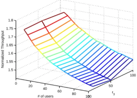
100 101 102 0 2000 4000 6000 8000 10000 12000 N=1200, E 1 = 10, Eh=1, and Em=0The desired number of electing cluster heads (n)
Network Lifetime (L) LEACH Scheme 1 Scheme 2a Scheme 2b Scheme 3
(2) 頻譜機會確認之機制
在今年的研究中,我們分析了一個感知無線網路在一定的區域範圍中所存在的機率,
同時也探討感知無線網路在屏避效應下的可靠性,最後我們利用 CSMA/CA 的通訊協定為
例子,分析出此種網路的總傳輸量
根據上面分析模型中所到的性能分析,我們可以歸納出一些感知無線網路的現象:
(a) 感知無線網路中兩種網路共同存在的機率對於上傳的基礎設施網路連線的主要使
用者位置相當敏感,
(b) 然而對於下傳的連線而言,無論主要使用者的位置為何,其網路共同存在的機率及
總傳輸量均是穩定的,
(c) 遮蔽效應並不會影響感知無線網路存在機率,然而由於訊號強度受到屏避效應的改
變,使得連線的可靠度會因位置而有巨幅的變化,
(d) 由於遮蔽效應的影響,感知無線電設備需要地點和通道狀態資訊來獲得足夠的資料
在適當的時間與地點建立網路連線。
在未來的研究中,我們將根據今年所觀察到的現象,設計一套通訊協定讓感知無線電設備
得以隨時隨地建立一個隨意網路連線,同時不干擾到主要使用者的傳輸。
相關論文發表
[1]
Li-Chun Wang, Chung-Wei Wang, and Chuan-Ming Liu, “Adaptive Contention
Window-based Cluster Head Election Algorithms for Wireless Sensor Networks,” VTC'05
Fall, vol. 3, pp. 1819-1823, September 2005.
[2] Li-Chun Wang, and Anderson Chen, “On the Coexistence of Infrastructure-Based and Ad Hoc
Connections for a Cognitive Radio System,” to be appeared in CrownCom 2006.
參考文獻
[1] W. B. Heinzelman, A. Chandrakasan, and H. Balakrishnan, “An Application-Specific Protocol
Architecture for Wireless Microsensor Networks," IEEE Transactions on Wireless
Communications, vol. 1, no. 4, pp. 660-670, October 2002.
[2] M. Handy, M. Haase, and D. Timmermann, “Low-Energy Adaptive Clustering Hierarchy with
Deterministic Cluster-Head Selection," 4th IEEE International Conference on Mobile and
Wireless Communications Networks, pp. 368-372, September 2002.
[3] L. Zhao, X. Hong, and Q. Liang, “Energy-Efficient Self-Organization for Wireless Sensor
Networks: A Fully Distributed Approach," Globecom 2004, December 2004.
[4] A. Depedri, A. Zanella, and R. Verdone, “An Energy Efficient Protocol for Wireless Ad Hoc
Sensor Networks," IEEE AINS'2003, pp. 1-6, June-July 2003.
[5] G. Smaragdakis, I. Matta, and A. Bestavros, “SEP: A Stable Election Protocol for clustered
heterogeneous wireless sensor networks," Second International Workshop on Sensor and
Actor Network Protocols and Applications, August 2004.
[6] H. Chan and A. Perrig, “ACE: An emergent algorithm for highly uniform cluster formation,"
European Workshop on Wireless Sensor Networks (EWSN 2004), pp. 154-171, January 2004.
[7] O. Younis and S. Fahmy, “HEED: A Hybrid, Energy-Efficient, Distributed Clustering
Approach for Ad-hoc Sensor Networks," IEEE Transactions on Mobile Computing, vol. 3, no.
4, pp. 366-379, October-December 2004.
[8] D. Cabric, S. M. Mishra, and R. W. Brodersen, “Implementation issues in spectrum sensing
for cognitive radios,” in Conference on Signals, Systems, and Computers, vol. 1, Nov. 2004,
pp. 772–776.
[9] T. Weiss, J. Hillenbrand, A. Krohn, and F. K. Jondral, “Mutual interference in OFDM-based
spectrum pooling systems,” in IEEE Vehicular Technology Conference, vol. 4, May 2004, pp.
1873–1877.
[10] M. Oner and F. Jondral, “Extracting the channel allocation information in a spectrum
pooling system exploiting cyclostationarity,” in IEEE Internation Symposium on Personal,
Indoors, and Mobile Radio Communications, vol. 1, Sep. 2004, pp. 551–555.
[11] F. Capar, I. Martoyo, T. Weiss, and F. Jondral, “Comparison of bandwidth utilization for
controlled and uncontrolled channel assignment in a spectrum pooling system,” in IEEE
Vehicular Technology Conference, vol. 3, May 2002, pp. 1069–1073.
[12] B. Aazhang, J. Lilleberg, and G. Middleton, “Spectrum sharing in a cellular system,” in
IEEE International Symposium on Spread Spectrum Techniques and Applications, Aug. 2004,
pp. 355–359.
[13] F. Capar, I. Martoyo, T. Weiss, and F. Jondral, “Analysis of coexistence strategies for
cellular and wireless local area networks,” in IEEE Vehicular Technology Conference, vol. 3,
Oct. 2003, pp. 1812–1816.
[14] T. Weiss, M. Spiering, and F. K. Jondral, “Quality of service in spectrum pooling systems,”
in IEEE Internation Symposium on Personal, Indoors, and Mobile Radio Communications,
vol. 1, Sep. 2004, pp. 345–349.
[15] H. Wu, C. Qiao, S. De, and O. Tonguz, “Integrated cellular and ad hoc relaying systems:
iCAR,” IEEE Journal on Selected Areas in Communication, vol. 19, no. 10, pp. 2105–2115,
Oct. 2001.
[16] E. Yanmaz, O. K. Tonguz, S. Mishra, H. Wu, and C. Qiao, “Efficient dynamic load
balancing algorithms using icar systems: a generalized framework,” in IEEE Vehicular
Technology Conference, vol. 1, Sep. 2002, pp. 586–590.
[17] E. H.-K. Wu, Y.-Z. Huang, and J.-H. Chiang, “Dynamic adaptive routing for heterogeneous
wireless network,” in IEEE Global Telecommunications Conference, vol. 6, Nov. 2001, pp.
3608–3612.
[18] Y. D. Lin and Y. C. Hsu, “Multihop cellular: a new architecture for wireless
communications,” in IEEE INFOCOM, vol. 3, Mar. 2000, pp. 26–30.
[19] J. Chen, S.-H. G. Chan, J. He, and S. C. Liew, “Mixed-mode WLAN: the integration of
ad-hoc mode with wireless LAN infrastructure,” in IEEE Global Telecommunications
Conference, vol. 1, Dec. 2003, pp. 231–235.
Adaptive Contention Window-based Cluster Head
Election Mechanisms for Wireless Sensor Networks
Li-Chun Wang
∗, Chung-Wei Wang
∗, and Chuan-Ming Liu
+,
∗
National Chiao Tung University, Taiwan
+
National Taipei University of Technology (NTUT), Taiwan
Email : [email protected]
Abstract— The clustering architecture is essential in achieving the goal of energy efficiency for a wireless sen-sor network. In general, a clustering algorithm consists of the cluster head election and the cluster member as-signment mechanism. This paper proposes an adaptive contention window (ACW)-based cluster head election mechanism. Unlike other legacy cluster head election mechanisms such as LEACH (Low Energy Adaptive Clustering Hierarchy) protocol, the proposed ACW algorithm can achieve four major goals in cluster head election for wireless sensor networks: 1) high successful probability of cluster head election, 2) appropriate number of cluster heads, 3) uniform distribution of cluster heads, and 4) equal times to be a cluster head for each sensor, simultaneously.
I. Introduction
To design a cluster-based wireless sensor network (WSNs), a basic problem is how to distributively organize a larger number of sensor nodes into different clusters. In WSNs, in order to achieve the objective of energy-efficiency, the cross-layer design is necessary to achieve energy saving in each sensor node [1]. In general, a cluster formation algorithm consists of the cluster head election and the member assignment mechanism. In this work, we focus on the cluster head election problem in WSNs.
The major goals of a cluster head election are four folds. We define the lifetime of a sensor network to be the time elapsed between the start of the system and the death of
the first node (FND). First, the successful probability of
head election must be as high as possible in order to save energy. Second, the number of elected cluster heads should be appropriate to enhance the network reliability. Third, the distribution of heads should be uniform. Fourth, each sensor node should becomes a cluster head with the same
times in order to even the energy consumption. When
the energy consumption is evened among all sensor nodes, no sensor node consumes more energy than other ones. Therefore, the lifetime can be extended.
In this paper, we propose an adaptive contention win-dow (ACW)-based cluster head election mechanism to guarantee these four concerns simultaneously. The legacy cluster head election mechanisms such as LEACH (Low
The work was supported jointly by the National Science Council and the MOE program for promoting university excellence under the contracts EX-91-E-FA06-4-4, 93-2219-E009-012, and 93-2213-E009-097.
Energy Adaptive Clustering Hierarchy) protocol [2], only focuses on the forth concern, i.e., the equal times to be a cluster head for each sensor. We compare three different schemes based on the ACW-based head election algorithm: the short-term fairness, the medium-term and long-term fairness schemes. We simulate the upper bound and the lower bound of the lifetimes in the proposed ACW algorithm. From our results, we find that the short-term fairness scheme of ACW algorithm performs better than the medium-term and long-term fairness schemes of ACW algorithm in terms of network lifetime.
The rest of this paper is organized as follows. In Section II, we analyzes the performance of head election in LEACH protocol. Section III shows our ACW-based cluster head election mechanism. Section IV analyzes ACW’s designing principle and shows some numerical results. Finally, we give our concluding remarks in Section V.
II. Motivation and Cluster Head Election Criteria
In this section, we discuss the design criteria for the cluster head election. For comparison, we analyze the performance of the head election algorithm in LEACH protocol. It is well know that the LEACH protocol can only guarantee the equal times to be heads for each sensor node. However, LEACH protocol cannot simultaneously guarantee the other concerns during the process of head election.
A. Background on the Head Election Mechanism in LEACH Protocol
In the LEACH protocol, each sensor node become the cluster head according to the probability related to the accumulative times of not being head before this round.
The ith sensor in rthround be head with probability:
Ti(r) = ( P 1−P ∗(r mod 1 P) , Ci(r) = 1 0 , Ci(r) = 0 (1) where P is the desired percentage of cluster heads among all sensor nodes in the entire network, r ∈ [0, ∞] is the current round if the holding energy of each sensor node
is infinite, and Ci(r) is the indicator function determining
whether the ith sensor node had been head in recent (r
cluster cluster head in most recent r modulo 1/P rounds).
In the (1
P − 1)thround, all sensor nodes that have not yet
been head set the value of Ti(r) be 1. Therefore, all of
them will be the heads in this round. After the (1
P − 1)th
round, the cluster heads are elected among all sensor nodes according to (1) once again.
Assume that the number of sensor nodes in the entire network is N . Hence, the value of P in (1) is equal to
n/N , where n is the desired number of electing cluster
heads. Let the value of k be (r modulo 1/P ) where
k ∈ [0,N
n − 1]. Then, the probabilities that sensor nodes
in kth competition are the same for different k. Next,
according to the following lemma 1, we can obtain the probability that there are j cluster heads are elected in
the kthcompetition.
Lemma 1: Suppose that there exists a game with N participants. The rules of game are described as follows: In each round, the participants firstly pick a number from the interval between [0, 1] randomly based on the uniform distribution. Then the participants whose picked number is less than a certain threshold can leave this game in this
round. The threshold is defined as P
1−P k, where k is the
times of round (k ∈ [0,1−P
P ]), and P is a constant between
[0, 1]. In the final round (k = 1−P
P ), the participants that
have not yet leaved before (1−P
P )th round can leave in
(1−P
P )th round because the threshold is set to 1 in this
round. In such a game, j participants leave the game in
kth round with probability¡N j
¢
Pj(1 − P )N −j. Notice that
the probability is independent of k. ¥
According to Lemma 1, there are j cluster heads are elected in each competition with probability:
P (j) = µ N j ¶ ³n N ´j³ 1 − n N ´N −j . (2)
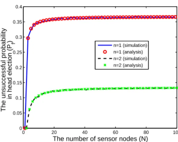
B. The Unsuccessful Probability in Head Election
From (2), the probability with no head elected (denoted
by Pf) is equal to
Pf= P (0) = (1 − n
N)
N . (3)
The unsuccessful probability of head election decreases as the desired number of electing cluster heads (n) increases. If the value of n approaches to N , the average unsuccessful probability will approach to zero. However, the value of n does not approach to N in WSNs, because the number of cluster members (N − n) should be larger than cluster
heads (n) in general (i.e., the value of n is less than N
2).
For example, in an extreme case when only cluster is required n = 1 and N approaches to infinite, it is followed that
lim
N →∞Pf = e
−1 . (4)
According to (4), in WSNs with larger amount of sensor nodes, the unsuccessful probability in head election is very significant under this case. Once the head election fails, sensor nodes either transmit data directly to sink or execute cluster head election algorithm again. Both situations consume a lot of energy.
0 20 40 60 80 100 0 0.05 0.1 0.15 0.2 0.25 0.3 0.35 0.4
The number of sensor nodes (N)
The unsuccessful probability
in head election (P f ) n=1 (simulation) n=1 (analysis) n=2 (simulation) n=2 (analysis)
Fig. 1. The unsuccessful probability (Pf) in head election for the
different value of N .
Figure 1 illustrates the unsuccessful probability of head election against the total number of sensor nodes N. As N
increases, Pf increases and saturates at 0.36 for n = 1. For
a larger value of n, although Pf decreases, a lager value
of n can lead to other problems as discussed in following sections.
C. Probability of Inaccurate Number of Elected Heads
An appropriate number of elected cluster head is also an important criteria for sensor network. With more redun-dant cluster heads, it may induce extra load to the sink and increase the difficulty of code orthogonality when the cluster heads adopt the code division multiple access to connect to the sink as considering in the LEACH protocol. On the other hand, with fewer cluster head as the designed value, the cluster head will be overloaded by extra cluster members. Let λ be the marginal percentage of the number of elected heads different from the designed value. Then, the probability that the number of the elected cluster heads is outside the acceptable range [d(1 − λ)ne, b(1 +
λ)nc] (denoted by Pu) becomes Pu= d(1−λ)ne−1X j=1 P (j) + N X j=b(1+λ)nc+1 P (j) . (5) where bxc and dxe are the operator to choose the largest integer less than x and the smallest integer larger than x, respectively.
Figure 2 shows the probability Pu against different
values of n. Firstly, when λ = 0.1, the probabilities
Pu = 0.5732 and 0.3891 for n = 20 and n = 60,
respectively. Thus, it is preferable to elect more heads in this consideration. On the other hand, for the case
that λ = 1.5, Pu = 0.4297 and 0.2078 for n = 20
and n = 60, respectively. Thus, when lesser heads are elected, the probability of inaccurate number of heads is also increases, thereby damaging the network reliability. Furthermore, when λ = 0 which means that network does not allow any inaccuracy on the number of elected heads,
0 20 40 60 80 100 120 0 0.1 0.2 0.3 0.4 0.5 0.6 0.7 0.8 0.9 1 n P u N=1200 λ=0 λ=0.1 λ=0.15
Fig. 2. Probability of inaccurate number of elected heads.
this case, lesser n has higher performance. In general, we hope the number of electing heads can be bounded in a certain range.
D. The Probability of Sufficient Separation Distance
By distributing the cluster heads uniformly, a sen-sor network can extend the lifetime. Furthermore, in an area with crowded cluster heads, the interference become higher. On the other hand, in an area with sparse cluster heads, the loading of each head become heavy because it has to manage more members. Therefore, the performance and energy efficiency of sensor networks degrade. To judge how the cluster heads are uniformly distributed in LEACH protocol, we need the following lemma.
Lemma 2: Suppose that X1, X2, Y1, and Y2are random
variables uniformly distributed in [−L
2,L2]. Let H = (X1−
X2)2+ (Y1− Y2)2. Then the probability density function
of Z can be derived as follows:
fH(h) = π 4L2 , 0 ≤ h ≤ L2 sin−1(1 − 2L2 z ) 2L2 , L2≤ z ≤ 2L2 . (6) ¥ Assume that all sensor nodes are uniformly deployed in
a squared area with vertex coordinates (L
2,L2), (L2, −L2),
(−L
2, −L2), and (−L2,L2). According to (1), each sensor
node that have not yet been the cluster head will become the cluster head with the same probability. Consider ζ
elected heads and let η =¡ζ2¢. Then the probability of the
square of separation distance between two cluster heads
being located at (X1, Y1) and (X2, Y2) is larger than d2
becomes P rob(Z > d2) = ÃZ 2L2 d2 fZ(z)dz !η , (7)
where Z = (X1− X2)2+ (Y1− Y2)2 and X1, X2, Y1, and
Y2 are uniformly distributed in [−L2,L2].
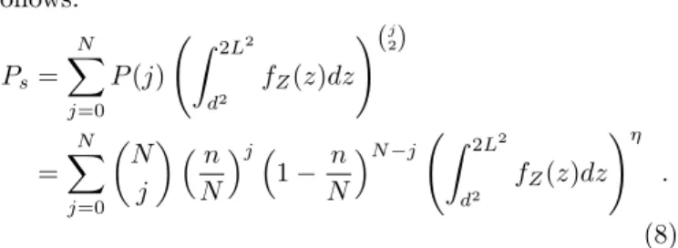
Now we calculate the average probability of the square
of separation distance larger than d2 (denoted by P
s) as follows: Ps= N X j=0 P (j) ÃZ 2L2 d2 fZ(z)dz !(j 2) = N X j=0 µ N j ¶ ³n N ´j³ 1 − n N ´N −jÃZ 2L2 d2 fZ(z)dz !η . (8)
Note that as n increases the probability Ps decreases.
Hence, the issue of non-uniform distribution for cluster heads becomes more severe.
E. Discussion
From the above analysis, we find that it is difficult for the LEACH protocol to simultaneously achieve the goals
of low unsuccessful probability in head election Pf, low
probability of inaccurate number of cluster head Pu, and
high probability of sufficient separation distance Ps.
We summarize some key observations:
• For n ≥ 2, we find that the larger the value of n, the
lower probability of sufficient separation Ps.
• For n = 1, although Ps is satisfactory, the
unsuccess-ful probability in head election Pfand the probability
of the inaccurate number of cluster heads Pu become
higher.
In summary, based on the above observation, we are motivated to propose a new head election mechanism to
achieve the design goals for sensor network in terms of Pf,
Pu, Ps, and the times of being cluster head, simultaneously
.
III. ACW-based Cluster Head Election Mechanism
In this section, we propose an adaptive contention window (ACW) mechanism to elect cluster heads. The main idea behind the proposed ACW-based head election mechanism is that all sensor nodes randomly pick a backoff value from the contention window based on the uniform distribution, and then the sensor node with the minimal backoff value can be cluster head in its communication range. In such a mechanism, ACW can rotatively elect cluster head, avoid the non-uniform distribution of cluster heads, bound the number of elected heads, and guarantee that a sensor node is elected to the cluster head at least
during each round (i.e. Pf = 0).
A. System Model
In our system model, we assume that all sensor nodes are synchronized by a certain synchronization mechanism [3]. In the beginning of each round, all sensor nodes em-ploy an existing contention-based medium access control (MAC) protocol to contend the channel. If the channel contention is successful, then the sensor node becomes a cluster head. Next, the cluster heads continuously transmit a signal to recruit other sensor nodes to be its member in order to form a cluster. If the state between the
request node and the response node satisfies with a certain criterion such as distance or receiving power constraints, the response node will confirm the request node and then become a member of this request node. Then, the cluster head will response the scheduling policy to its members [4].
To explain the basic concept, we consider an area with three sensor nodes A, B and C, among which one cluster head is elected. First, all sensor nodes pick a backoff value from the contention window randomly based on the uniform distribution. Then the sensor node with the minimal backoff value become a cluster head.
B. Scheme 1 (long-term fairness based):
On the beginning, sensors A, B and C have the same contention window size denoted as [0, CW − 1]. Assume that sensor A has minimal backoff value picked from [0, CW − 1] uniformly. Then sensor A become the cluster head in this round. In the following rounds, all sensor nodes pick backoff value from [0, CW −1] again. In the long run, the rotation of cluster heads achieves the long-term fairness. In scheme 1, one key designing problem is how to decide the initial value of CW , which will be discussed later.
C. Scheme 2 (medium-term fairness based):
First, sensors A, B and C have the same contention window [0, CW − 1]. Let sensor A be the cluster head in the first round. After being the cluster head, sensor A increases its contention window size to CW + 2 in order to decrease the probability of being the cluster head again in the next round. In the meanwhile, B and C decrease their contention window size to CW − 1 in order to increase the probability of being cluster head in next round. In the second round, sensor A pick the backoff value from [0, CW + 1], and B and C pick the backoff value from [0, CW − 2], respectively. In the following rounds, in order to dynamically change the probability of being the cluster head, all sensor nodes adjust the value of their
CW s according to whether they have been heads or not.
By dynamically adjusting the contention window size, the rotation of heads is more fair than Scheme 1. In this scheme, one key designing problem is to determine the adaptation size in contention window.
D. Scheme 3 (short-term fairness based):
Let sensors A, B and C have the same contention window [0, CW − 1] on the beginning. If sensor A is the cluster head in first round, sensor A will not participate in the contention of cluster head election until all sensor nodes have been the cluster heads exact once. Then, in the second round, only sensors B and C compete each other, and pick a backoff value from [0, CW − 2]. Therefore, the rotation of heads is more fair than Scheme 2, and we call it short-term fairness. In this scheme, one key designing problem is why we should decrease the value of CW by one.
E. Discussion
The above three ACW-based schemes can fulfill the four major design goals of head election mechanism. First, since the backoff value eventually will become zero, it is ensured that a sensor node will be elected as the cluster head at least once. Second, in the ACW-based head election mechanism, the carries sense and broadcast mechanisms can make any two cluster heads maintain suitable distance. Third, due to the carrier sense and broadcast mechanisms, the number of cluster heads can also be automatically converge to a suitable range. Forth and the last, because the ACW-based method adapts the window size depending on the fairness requirement, each sensor node becomes the cluster head with about the same times.
IV. Design of the Contention Window Size for Cluster Head Election
In this section, we explain how to adjust the value of
CW for the ACW-based cluster head election mechanism. A. Scheme 1
According to [5], when the value of CW is equal to the number of sensor nodes (denoted by N ), the average head election time (t) can be minimized. The head election time (t) can be estimated as follows. First, the probability of only one sensor node in an area with N sensor nodes accessing the channel is calculated by
PS=
µ
N
1 
Prob{a sensor picks a particular time slot out of CW time slots}·
Prob{other sensor nodes pick other time slots} = µ N 1 ¶ 1 CW × (1 − 1 CW) (N −1) . (9)
For CW = N , it is followed that
PS > e−1 . (10)
Thus, the probability of unsuccessful head election in t continuous time slots become
(1 − PS)t< (1 − e−1)t . (11)
That is, the probability that Scheme 1 can elect a cluster
head during t time slots is at least 1 − (1 − e−1)t.
B. Scheme 2
The principle of Scheme 2 is to make the probability of being cluster head for each sensor node proportionated to
its remained energy. Denote Ei,r and CWi,r the current
remained energy and the CW value for the ith sensor in
the rth round, respectively. Because a sensor node with
more remained energy should be assigned with a smaller value of CW , we can have
CWi,r= d
PN
j=1Ej,r
where dxe is the operator to choose the smallest integer
larger than x. Now, we explain how to estimatePNj=1Ej,r.
Let E0, Eh, and Em be the average initial energy, the
average energy consumption for a cluster head in each round, and the average energy consumption for a cluster member in each round, respectively. Then
N X i=1 Ei,r ≈ (N − 1)E0 | {z } term 1 − [(r − hi,r)Eh+ (N − 1)hi,rEm] | {z } term2 + Ei,r |{z} term3 , (13)
where hi,r is the times that ithsensor has been the cluster
head in r rounds. In (13), term 1 is the sum of the initial energy of other N − 1 sensor nodes, and term 2 is the energy consumption of other (N − 1) sensors in r round. Note that (13) can be obtained distributively at each sensor node.
C. Scheme 3
In this scheme, all the sensor nodes decrease their CW value by one in each round, while the current cluster head sets its CW value to be an infinite number in the next round. The idea of this scheme is to ensure that a sensor node will not be the cluster head more than once in N rounds.
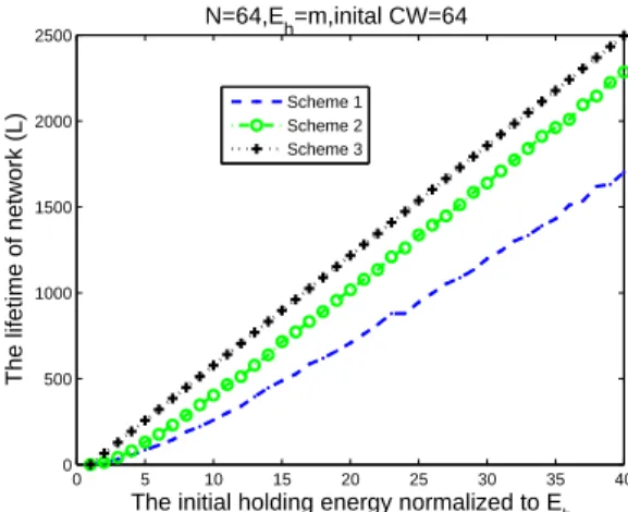
D. Performance Comparison
Figure 3 compares the lifetime of the three different
schemes against different initial energy normalized to Eh.
The three schemes differ in how we set the window size
CW . Scheme 1 does not need to adjust the value of CW
over rounds. Therefore, it is the simplest scheme and also has shortest lifetime. In Scheme 2, sensor nodes decrease or increase the value of CW depending whether a sensor node is the cluster head in this round. In Scheme 3, sensor nodes are rotated to serve the cluster head. This scheme has the longest lifetime among the three considered ACW-based head election mechanisms.
V. Conclusions
In this paper, we have discussed the cluster head election issue. We have identified the four major goals to design the cluster head election mechanisms: 1) high successful probability of cluster head election, 2) appropriate number of cluster heads, 3) uniform distribution of cluster heads, and 4) equal times to be a cluster head for each sensor, simultaneously. With respect to the above four objectives, we find that the legacy LEACH protocol does not fulfill the first three gaols very well.
Thus, we propose the adaptive contention window (ACW) based head election mechanisms. The proposed ACW-based head election mechanisms employ the carrier sense multiple access (CSMA) MAC protocol with backoff procedures. Thanks to the the backoff procedure, the
0 5 10 15 20 25 30 35 40 0 500 1000 1500 2000 2500 N=64,Eh=m,inital CW=64
The initial holding energy normalized to E
h
The lifetime of network (L)
Scheme 1 Scheme 2 Scheme 3
Fig. 3. The lifetime comparison of different schemes for the different initial holding energy normalized by Eh.
first can be fulfilled. Furthermore, the carrier sensing capability can achieve the second and the third goals. By mapping the remained energy in each sensor node to the contention window size, the forth goal can be achieved. We also compare three kinds of ACW-based head election mechanisms and discuss how to set the contention window size to achieve different fairness requirements.
In this paper, we have only qualitatively demonstrated the effectiveness of the proposed ACW-based head election mechanisms. One of our undergoing work is to analytically prove the proposed ACW-based mechanisms can achieve the four design goals for electing head in wireless sensor networks.
References
[1] I. F. Akyildiz and I. H. Kasimoglu, “Wireless Sensor and Actor Networks: Research Challenges,” Ad Hoc Networks Journal, pp. 351–367, May 2004.
[2] W. B. Heinzelman, A. Chandrakasan, and H. Balakrishnan, “An Application-Specific Protocol Architecture for Wireless Mi-crosensor Networks,” IEEE Transactions on Wireless
Communi-cations, vol. 1, no. 4, pp. 660–670, October 2002.
[3] S. Ganeriwal, R. Kumar, and M. B. Srivastava, “Timing-sync Protocol for Sensor Networks,” in Proceedings of the first
interna-tional conference on Embedded networked sensor systems. ACM
Press, November 2003, pp. 138–149.
[4] L.-C. Wang, C.-W. Wang, and C.-M. Liu, “A Cross-Layer Design for Determining the Optimal Number of Clusters in a Wireless Sensor Network,” International Conference on Computing,
Com-munications and Control Technologies (CCCT), pp. 269–274,
August 2004.
[5] I. Stojmenovic, Ed., Handbook of Wireless Networks and Mobile
On the Coexistence of Infrastructure-Based and Ad Hoc Connections for a
Cognitive Radio System
1Li-Chun Wang
∗and Anderson Chen
National Chiao Tung University, Hsin-Chu, Taiwan
Abstract
Cognitive radio (CR) can sense the current spectrum us-age of existing networks and make intelligent decisions on the opportunity of reusing the frequency spectrum. One fun-damental issue for the CR system is how to rapidly establish a temporary communication link on the spectrum of the ex-iting users. In this paper, we investigate the feasibility issue of establishing both an infrastructure-based link and an ad hoc link using the same spectrum simultaneously in an over-lapped area. We also present a cross-layer performance analysis from both the physical (PHY) layer and medium access control (MAC) layer perspectives. The analytical re-sults show that the probability that both an infrastructure-based connection and an ad hoc link coexist in an overlap-ping area can be as high as 45%. In addition, the normal-ized total throughput of the both links is more than 145% compared to the pure infrastructure-based link. However, considering the shadowing effects, the transmission relia-bility varies from 30% ∼ 90% depending on the locations of mobile stations.
1
Introduction
Cognitive radio (CR) is an important research topic in recent years due to the efficient usage of licensed spectrum at anywhere and in anytime [6, 1]. A CR device senses the surrounding environment and adjusts the transmission parameters to establish an unharmful communication link to the existing legacy systems. The key enabling technologies for a CR device include [6, 1, 7]:
• sensing a wide spectrum range;
• identifying the spectrum usage of primary users in
terms of transmit power, locations and time;
• realizing the opportunities of sharing the spectrum
with the existing primary users.
For the first goal, the authors in [3, 9] discussed the spec-trum sensing issues from the viewpoint of signal process-ing. For the second goal, in [4, 2], the authors proposed a spectrum usage model of the primary users to help the CR-enabled users identify the available spectrum in terms of time. The objective of this paper is to achieve the third goal, i.e. to examine the opportunity of spectrum reuse of
1This work was supported by the National Science Council, Taiwan
under the contract NSC94-2213-E-009-060.
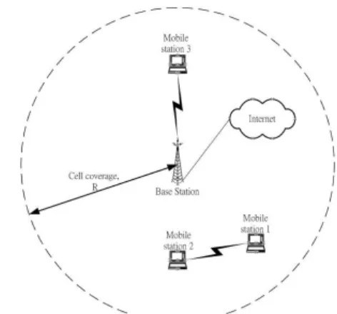
Figure 1. An example for the coexistence of two CR-enabled devices establishing an ad hoc link and a legacy user connecting to the infrastructure-based network, where all devices use the same spectrum at the same time.
the existing infrastructure-based users for the CR-enabled device to establish a peer-to-peer ad hoc connection in term of location.
Although many studies have been reported in the lit-erature on the subject of the coexistence of the hybrid infrastructure-based and ad-hoc networks [12, 8, 5], they may not be directly applied for the CR system. In [12, 8], the idea of combining ad hoc link and infrastructure-based link was proposed to extend the coverage area of the infrastructure-based network. The coverage area of the in-frastructure and ad hoc links were not overlapped; while in a CR network, both the links coexist in an overlapped area. In [5], it was demonstrated by simulations that the throughput of a wireless local area network (WLAN) can be improved if an access point (AP) can instruct the user to switch be-tween the infrastructure mode and the ad hoc mode. How-ever, a CR-enabled device is required to establish an ad hoc connection in a distributed manner.
In this paper we investigate the feasibility of establish-ing an ad hoc link with an existestablish-ing infrastructure connec-tion using the carrier-sense multiple access with collision avoidance (CSMA/CA) medium access control (MAC) pro-tocol. We also develop a cross-layer analytical model to evaluate the throughput performance of both the links in an overlapping area. The results show that more than 45% probability the both links can coexist, and more than 145% throughput performance can be obtained compared to the pure infrastructure-based link.
Figure 2. The physical representation for the coexistence probability for a CR-based ad hoc connection and the uplink infrastructure-based connection.
2
System Model and Propagation Model
Figure 1 shows an example where two CR-enabled devices making a peer-to-peer ad hoc connection (MS1 to MS2) coexist with the legacy user connecting to the infrastructure-based wireless network (MS3 to AP). Sup-pose that at any instant only one peer-to-peer ad hoc con-nection and one infrastructure-based link can be established inside the cell coverage. We define the coexistence proba-bility of both the connections in an overlapping area as
PCR= P {(SIRi> zi) ∩ (SIRa > za)}, (1)
where SIRi and SIRa denote the received
signal-to-interference ratios (SIRs) of the infrastructure-based and ad hoc links, respectively; zi and za are the required SIR
thresholds for the infrastructubased and ad hoc links, re-spectively.
Moreover, we consider the following propagation model for the SIR calculations [10]:
Pr=
Pth2aph2msGapGms
rα , (2)
where Prand Ptare the received and transmit power of a
mobile station; hapand hmsrepresent the antenna heights
of the access point and the mobile station; Gap and Gms
stand for the antenna gains of the access point and the mo-bile station; r is the propagation distance between the trans-mitter and the receiver; and α = 4 is the path loss exponent.
3
Physical Layer SIR Analysis
Assume MS1 is uniformly distributed in the cell of ra-dius R and locates at (r1, θ1); the locations of AP, MS2 and MS3 are (0, 0), (r2, θ2) and (r3, θ3). The coexistence prob-ability PCRcan be calculated as follows.
3.1
Uplink SIR Analysis
In the uplink case, the legacy infrastructure-based user MS3 transmits data to the AP. Denote P30 and P10 the received power from MS3 and that from MS1 at the AP, respectively. From (2), the uplink SIR of the legacy infrastructure-based network (i.e. MS3 → AP) can be ex-pressed as SIRi= P30 P10 = ( r1 r3) α , (3)
where r1and r3are the distances between AP to MS1 and MS3, respectively. Similarly, we can express the SIR of a CR-based peer-to-peer ad hoc link from MS1 to MS2 as
(a) max(r+, r−) ≤ R.
(b) max(r+, r−) > R.
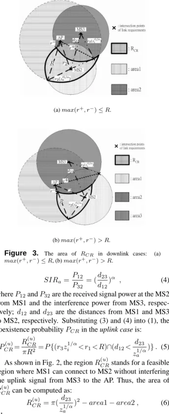
Figure 3. The area of RCR in downlink cases: (a) max(r+, r−) ≤ R, (b) max(r+, r−) > R. SIRa= P12 P32 = ( d23 d12) α , (4)
where P12and P32are the received signal power at the MS2 from MS1 and the interference power from MS3, respec-tively; d12 and d23 are the distances from MS1 and MS3 to MS2, respectively. Substituting (3) and (4) into (1), the coexistence probability PCRin the uplink case is:
PCR(u)=R (u) CR πR2 = P {(r3z 1/α i < r1< R)∩(d12< d23 z1/αa )} . (5) As shown in Fig. 2, the region RCR(u) stands for a feasible region where MS1 can connect to MS2 without interfering the uplink signal from MS3 to the AP. Thus, the area of
R(u)CRcan be computed as:
RCR(u) = π(d23 za1/α )2− area1 − area2 , (6) where area1 = (d23 za1/α )2(π − θ0) − R2θ + 2∆ ; (7) area2 = (d23 za1/α )2φ − (r 3zi1/α)2φ0− 2∆0. (8)
The definitions of parameters θ, θ0, φ, φ0, ∆, and ∆0 and the detail derivation of (6), (7) and (8) will be detailed in our journal version due to the page limit.
3.2
Downlink SIR Analysis:
In the downlink case, the AP always sends data to the legacy user MS3 through the infrastructure link. From (2), the SIR of the infrastructure link can be written as:
SIRi= P03 P13 = ( hap hms) 2(d13 r3 ) α , (9)
where P03and P13are the received power from the AP and that from MS1 at MS3, respectively; d13stands for the dis-tance between MS1 to MS3; hap, hms and r3are given in (2) and (3), respectively. Similarly, the SIR of the ad hoc link can be expressed as
SIRa= P12 P02 = ( hms hap) 2(r2 d12) α , (10)
where P12 and P02 are the received power at MS2 from MS1 and that from AP, respectively; r2represents the dis-tance between MS2 and the AP; hap, hms and d12 are de-fined in (2) and (4).
Substituting (9) and (10) into (1), we can obtain the co-existence probability of a CR-based ad hoc network PCRin
the presence of the infrastructure-based downlink transmis-sion as PCR(d)= R (d) CR πR2 = P {(d13> r3z01/αi ) ∩ (d12< r2za01/α) ∩ (r1< R)} , (11) where z0i = zih 2 ms h2 ap and z 0 a = z1a h2 ms h2
ap. Figure 3 shows the coexistence region R(d)CRin the downlink case according to (11). To compute the area of RdCR, we first denote r+and
r−as the distances from the AP to the intersection points of
the two circles of radius r3zi01/α and r2za01/α, respectively.
Then, r+and r−can be written as:
r+ = 1 d2 23 {r2r3[r2r3(z0 2 α a + z0 2 α i ) + sin(θ2− θ3)δ +cos(θ2− θ3)(d223− r22z 02 α a − r23z 02 α i )]} ; (12) r− = 1 d2 23 {r2r3[r2r3(z0 2 α a + z0 2 α i ) − sin(θ2− θ3)δ +cos(θ2− θ3)(d223− r22z 02 α a − r32z 02 α i )]} , (13) where δ = q 2r2 3z 02 α i (d223+r22z 02 α a )−(d223−r22z 02 α a )2−r43z 04 α i . (14)
Depending on the value of r+and r−, R(d)CRbecomes: 1. max(r+, r−) ≤ R: In Fig. 3(a), the area of R(d)CRis
R(d)CR= π(d23za01/α)2− area1 − area2 , (15)
where
area1 = (r2z01/αa )2(π − θ0) − R2θ + 2∆ ; (16) area2 = (r2za01/α)2φ − (r3z01/αi )2φ0− 2∆0. (17)
2. max(r+, r−) > R: In Fig. 3(b), the area of R(d)
CRis R(d)CR= π(d23za01/α)2−area1−area2+area3 , (18) where area1 = (r2za01/α)2(π − θ0) − R2θ + 2∆ ; (19) area2 = (r2za01/α)2φ − (r3z01/αi )2φ0− 2∆0; (20) area3 = ∆00+(r32zi02/αψ2− 1 2r 2 3z02/αi sin ψ2)+ (r22za02/αψ3− 1 2r 2 2z02/αa sin ψ3)−(R2ψ1− 1 2R 2sin ψ 1). (21)
The detailed derivations of (15) and (18) and the definitions of the parameters θ, θ0, φ, φ0, ψ1, ψ2, ψ3, ∆, ∆0, and ∆00 will be given in our journal version due to the page limit.
4
Shadowing Effects
In the following, we consider the shadowing impacts on the coexistence probability. Due to shadowing, the mobile station locating inside the region RCR in (6), (15) and (19)
may still fail to establish a peer-to-peer connection. Thus, we define F (PCR) as the reliability that the coexistence
probability PCRin the presence of shadowing:
F (PCR)=P {(SIRi> zi)∩(SIRa> z)|M S1 ∈ RCR}, (22)
where SIRiand SIRaare influenced by shadowing. Note
that F (PCR) = 1 when shadowing is not considered. We
can express F (PCR) for uplink and downlink cases subject
to shadowing as: • uplink case: F (PCR(u)) = P {(ξ30− ξ10> 10 log10(zi(rr31)α)) ∩(ξ12− ξ32> 10 log10(za(dd1223)α))|M S1 ∈ R(u)CR} ; (23) • downlink case: F (PCR(d)) = P {(ξ30− ξ13> 10 log10(zi(dr133)α)) ∩(ξ12− ξ02> 10 log10(za(dr122)α))|M S1 ∈ R(d)CR} . (24)
Recall that the shadowing component is a log-normally dis-tributed random variable and thus ξi,jis independent
Gaus-sian random variable with zero mean and the standard devi-ation of σξ. Assume that ξi,jhave the same standard
devi-ation for all i and j. Then, the difference between any two
ξi,j becomes a Gaussian random variable with N(0, 2σξ).
Therefore, F (PCR(u)) and F (PCR(d)) can be written
F (PCR(u)) = Q(10 log10zi( r3 r1) α 2√2σ )Q( 10 log10za(dd1223)α 2√2σ ) ; (25) F (PCR(d))=Q(10 log10zi( r3 d13) α 2√2σ )Q( 10 log10za(dr122 ) α 2√2σ ) , (26) where Q(x) = π1Rx∞exp−x2dx.
5
MAC Layer Throughput Analysis
In this section, the MAC layer throughput for the inte-grated networks with a CR-based ad hoc link and a legacy infrastructure connections is evaluated from a PHY/MAC cross-layer perspective. Assume that NCRCR-enabled
de-vices and N non-CR dede-vices are in the cell. Recall that the CR-enabled device can sense its surrounding environment and establish an additional ad hoc link without injuring the existing infrastructure-based connection. Therefore, the to-tal throughput of hybrid infrastructure and CR-based ad hoc
network SCR is contributed by the two parts, i.e. Siin the
infrastructure-based link and Sa in the ad hoc connection,
and thus S
CR= Si+ Sa. (27)
Assume the CSMA/CA MAC protocol is used to resolve the channel contention in both the infrastructure-based and peer-to-peer ad hoc links. In [11], the throughput S of the CSMA/CA MAC protocol with the channel impact and multiuser capture effect is expressed as
S = δ (1−pns(N ))E[P ]
1−(1−τ )N+(1−pns(N ))Ts+pns(N )Tc−δ
, (28) where N , E[P], Ts, Tc, and δ represent the number of
con-tending stations, average payload size, average successful transmission duration, average collision duration, and slot duration. τ and pns(N ) are the stationary transmission
probability and the failure probability in receiving a frame, respectively. The detail derivation can be found in [11].
From (28), the cross-layer analytical model can be applied to evaluate the throughput contributed from the infrastructure-based (Si) and CR-based ad hoc (Sa) links:
Si= δ (1−pns(N ))E[P ] 1−(1−τ )N+(1−pns(N ))Ts+pns(N )Tc−δ ; (29) Sa= (1−pns(N0))E[P ] δ 1−(1−τ )N 0+(1−pns(N0))Ts+pns(N0)Tc−δ , (30) where N0= NCRPCR.
For the infrastructure-based link, since N non-CR de-vices contend for establishing an infrastructure-based link with the AP, the throughput of infrastructure-based link Si
is the same as (28). However, for the CR-based ad hoc link, since an infrastructure-based connection already exists in the cell, only NCRPCR CR-enabled devices have the
op-portunity to establish an ad hoc link. Hence, the through-put of ad hoc link Sa is similar to (28), but the number of
contending stations in (28) becomes NCRPCR. Therefore,
substituting (29) and (30) into (27), we can consider the to-tal throughput of the CR network SCRas two independent
networks with different number of contending stations N and NCRPCR, respectively.
6
Numerical Results
In this section, we investigate the coexistence probability and the throughput performance of a hybrid CR-based ad hoc link and the infrastructure network.
6.1
Coexistence Probability
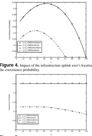
Figure 4 shows the impact of infrastructure uplink trans-mission on the coexistence probability of an ad hoc link and infrastructure-based link by changing the location of the infrastructure-based user MS3 within the entire cell. As shown in the figure, the coexistence probability versus the distance from MS3 to the AP is a convex curve. This phenomenon can be explained in two folds. On the one hand, when MS3 approaches AP, it is also closer to the CR-enabled ad hoc users, thereby causing high interference and
0 10 20 30 40 50 60 70 80 90 100 0 0.05 0.1 0.15 0.2 0.25 0.3 0.35 0.4 0.45 Coexistence Probability r 3 zi=za=0dB(simulation) zi=za=0dB(analysis) zi=za=3dB(simulation) zi=za=3dB(analysis)
Figure 4.Impact of the infrastructure uplink user’s location on the coexistence probability.
0 10 20 30 40 50 60 70 80 90 100 0 0.05 0.1 0.15 0.2 0.25 r3 Coexistence Probability z i=za=0dB(simulation) z i=za=0dB(analysis) zi=za=3dB(simulation) zi=za=3dB(analysis)
Figure 5.Impact of the infrastructure downlink user’s location on the coexistence probability.
decreasing the coexistence probability. On the other hand, when MS3 moves away from AP, the SIR of the infrastruc-ture link of MS3 also decreases due to higher path loss. Therefore, there exists an optimal location of MS3 that can lead to the maximal coexistence probability. In the consid-ered example, the maximal coexistence probability is 45% when the interferer MS3 is located at r=40 meters and the SIR threshold zi=za=0 dB. For zi=za=3 dB PCR=22.5%
when MS3 is posited at (30, π2).
Figure 5 shows the coexistence probability of the CR-based ad hoc connection versus the distance from MS3 to the AP. When zi=za=0 dB, the coexistence probability
re-mains constant (i.e. PCR=25%) as r ≤ 100 meters. That is,
the downlink interference from the AP to the ad-hoc links is independent of MS3’s locations in this case. Neverthe-less, with a more stringent SIR requirements, e.g. zi=za=3
dB, the coexistence probability slightly decreases as r3 in-creases.
6.2
Shadowing Effect on
PCRIn Fig. 6, comparing the reliability FCRwith σξ=1 dB
and 6 dB in both the downlink case (solid lines) and uplink case (dotted lines), the larger the shadowing standard devia-tion, the less the reliability of the mobile stations inside the
RCRregion. For example, as MS3’s locations change from r3=0 to r3=100 meters FCRis 90% for σξ=1 dB, and FCR
ranges between 60% to 70% for σξ=6 dB.
However, compared to the downlink case, the impact of shadowing on FCR is very significant for the uplink case