利用自發脈衝光引起光注入鎖模之二段式邊射型雷射高頻特性研究

國

立

交

通

大

學

影像與生醫光電研究所

碩

士

論

文

利用自發脈衝光引起光注入鎖模之二段式邊射型雷射高頻特

性研究

Monolithic Two-Section Self-Pulsation Edge Emitting Laser With Injection

Locking Technique

研 究 生：林智偉

指導教授：郭浩中 教授

盧廷昌 教授

中 華 民 國 一 百 年 七 月

利用自發脈衝光引起光注入鎖模之二段式邊射型雷射高頻特

性研究

Monolithic Two-Section Self-Pulsation Edge Emitting Laser With Injection

Locking Technique

研 究 生：林智偉 Student：Chih-Wei Lin

指導教授：郭浩中 Advisor：Hao-Chung Kuo

盧廷昌 Tien-Chang Lu

國 立 交 通 大 學

影像與生醫光電研究所

碩 士 論 文

A Thesis

Submitted to Institute of Imaging and Biomedical Photonics National Chiao Tung University

in partial Fulfillment of the Requirements for the Degree of

Master in

Imaging and Biomedical Photonics July 2011

Tainan, Taiwan, Republic of China

利用自發回饋引起光注入鎖模之二段式可調式雷射

學生：林智偉

指導教授：郭浩中

盧廷昌

國立交通大學影像與生醫光電研究所碩士班

摘

要

本論文中我們研究利用回饋引起光注入鎖模的二段式可調式雷射特性，發光波

長為 1.55 微米，我們使兩顆緊鄰的相同的雷射元件中央位置準確地利用聚焦離

子束與電子束蝕刻出具有特定寬度深度的空氣柱，此雷射一出光端面為高反射層

而另一端面為抗反射層，我們藉由共振腔光場強度的模擬結果可知主要由空氣柱

的深度變化導致由主雷射的共振腔產生的雷射光注入到副雷射共振腔的注入比

例不同，此外，主副雷射之間的電流分佈也隨著空氣柱的深度有所不同。我們基

於光注入鎖模理論，在一個穩定的光注入鎖模範圍內，顯示出分別在有外部注入

光與無外部注入光源的情況下做相對雜訊的量測與模擬，我們觀察到在有外部注

入光的情況下，雷射共振腔的共振頻率可以大幅提升。理論上若使得主雷射的光

注入比例越大，則共振頻率峰值可增加至 10 GHz 以上，另外利用此技術可使得

相對強度雜訊能夠有效的降低，在本論文中將由特定空氣柱深度的條件設定以及

鎖模情況下，改變主雷射的注入光比例使得相對強度雜訊峰值能夠至少達至 20

GHz。由此技術可使雷射大幅增加頻寬，頻譜分析與探討將在本論文中進行研究

與討論。

Monolithic Two-Section Self-Pulsation Edge Emitting Laser With

Injection Locking Technique

Student：

Chih-Wei Lin

Advisors：Dr.

Hao-Chung Kuo

Dr.

Tien-Chang Lu

Institute of Imaging and Biomedical Photonics

National Chiao Tung University

ABSTRACT

In this thesis,we study the characteristics of the 1.55μm two-section

self-feedfack laser with injection-locking technique.We fabricate an air

gap with a specific width and depth in the middle of the two single-mode

laser side by side with the focus ion beam system. The laser device has an

high-reflection facet and an anti-reflection one on the other side. From the

wave intensity simulation, we know that the injection ratio from the

master laser (ML) to the slave laser (SL) will differ at different depths.

Besides, the current distribution in the two-section cavity will also differ

because of the different depths.

Based on the optical injection-locking theory, we present the device

structure about 1.55µm two-section edge emitting laser、the relative

intensity noise (RIN) measurement of the device with light injection and

without light injection, and the simulation results of RIN spectrum .We

can observe that the resonance frequency increase largely under a

external injection light condition.

Theoretically if we increase the

injection ratio, the resonance frequency can be up to 10 GHz at least, and

relative intensity noise can reduce effectively. In this thesis fixing some

gap depths, we change the injection ratio from ML, and we can enhance

the RF frequency up to 20 GHz at least under injection-locking condition.

With the technique, we can increase the laser modulation bandwidth.

誌

謝

首先必須感謝指導教授郭浩中與盧廷昌老師半導體雷射實驗室給予我豐沛 的實驗資源，讓我無需擔心實驗事宜，然而最感謝的是林建中老師的對我實驗內 容的不厭其煩的親自督導與討論，每當遇到瓶頸時總給予適時的幫助以及給我正 確的方向解決問題，祝老師們研究順利，身體健康。 其次要感謝的是陳智弘老師與林俊廷老師實驗室對於我的實驗所需的軟硬 體部分全力支援，以及感謝何俊鴻博士生以及趙明義同學的居中協調與實驗儀器 教育訓練；感謝程育人老師實驗室的成員，也給予我適當的實驗協助，讓我的實 驗能夠順利進行。 感謝獸皇學長在我碩一下的時候教我實驗操作、還有珣文學姐、鏡學學長與 我在模擬上的討論、博孝學長的 DBR 鍍膜協助，感謝阿國、SGG、90 哥、Just、 幼齒、肉哥、家齊、翌臻、瑋婷、KaKa、峰瑜、冠霖、大寶、小杜、Joseph、板 弟、阿伯、信助、奇潁、威麟等等，以及台南校區光電學院第一屆的同學們，有 了你們的陪伴使我的碩士生涯多采多姿。 最後，感謝我的父母給予我全力的支持，讓我求學生涯無後顧之憂，讓我能 夠完成學業。 林智偉 2011/07/31 於交通大學

CONTENTS

Abstract(in Chinese)……….I

Abstract(in English)……… II

Contents………III

List of tables………VI

List of figures………..VII

Acknowledgement………

Chapter 1 Introduction………1

1.1 Light Sources On Optical Communication System……….1

1.2 Introduction of the Multisection Laser ………3

References..………5

Chapter 2 Theory……….………....6

2.1 Optical Injection Locking……….6

2.2 Theory Model………8

2.3 Linewidth enhancement factor………10

2.4 Simulation Theory………...12

2.5 Couple-Wave Equations………..15

2.6 Theory of Relative Intensity Noise(RIN)………19

Chapter 3 Simulation Result of the Self-pulsation Laser…………..25

3.1 Background On Design………..25

3.2 Wave intensity distribution analysis………..29

3-3.Two-Section Laser Simulation With Different Slot Depth…………33

3.3.1 L-I Curve ………33

3.3.2 Leakage Current ……….35

References………...….36

Chapter 4 Experiments Results………..37

4.1 Two-Section Laser Structure ……….37

4.2 FIB(focus ion beam) Etching Process………...……….39

4.3 Leakage Current Measurement………...41

4.4 Distributed Bragg Reflectors on Edge-laser HR facet………42

4.4.1 Introduction of Distributed Bragg reflectors………...42

4.4.2 Reflectance Simulation of T

i

O

2

/SiO

2

DBRs………..44

4.5 Optical Spectrum and RIN Measurement

4.5.1 Experimental Setup………46

4.5.2 Optical Spectrum Measurement Without FIB Process……..47

4.5.3 Optical Spectrum Measurement with an air gap…………....49

References………....56

List of Tables

Table1.Comparision of different lasing modes of laser devices………1

Table 2. Field intensity ratio on the pumped cavity……….31

Table 3.The resistance value between two top contacts………...41

Table 4.Mode spacing and RF frequency with weak injection………50

Table 5. Mode spacing and RF frequency with strong injection……….51

Table 6. Mode spacing and RF frequency of the injection-locked laser with strong injection………52

List of Figures

Figure 2.1.1 Optical Injection-Locking On Semiconductor Laser………7 Figure 2.1.2 Injection locking stability as a function of injection ratio R and frequency detuning Δf……….9 Figure. 3.1.1 Mode profile of the fundamental mode and refractive index profile

through the laser structure………25 Figure 3.1.2. Schematic description of single slot laser diode……….26 Figure 3.1.3 Calculated reflection spectrum of a single slot laser diode versus

wavelength operating near 1550 nm………....28 Figure 3.2.1. 2-dimensional simulation of pumped dual-section cavity………..30 Figure 3.2.2. Calculation of confinement of E-field in the quantum well axial

direction………30 Figure 3.2.3. (a) Field distribution: Wgap=5μm, but with no air gap; (b) Field

distribution on Wgap=5μm,Dgap=5 μm………..31

Figure 3.3.1.L-I curve (a) simulation results with different Dgap (b) measurement

result with Dgap=5um………33

Figure 3.3.2.Current distribution with different depths of the air gap……….35 Figure 4.1.1. 1.55μm InGaAsP Fabry-Perot laser with a tunable air gap in the middle section………..38 Figure 4.1.2. Typical experimental setups for edge-emitting laser as a slave laser….38 Figure 4.2.1 Dual beam (focused ion beam & electron beam) System (FIB/SEM)….39 Figure 4.2.2. SEM figure (Dgap is 5um.) ………40 Figure 4.3.1.I-V curve between the two top contacts………...41 Figure 4.4.1. distributed Bragg reflector………..42 Figure 4.4.2(a) TFCalc simulation and reflectivity measurement(~1000nm)(b)

reflectivity measurement(~2000nm)………45 Figure 4.5.1. experimental setup for measurement………..46 Figure 4.5.2.optical spectrum of two-section laser(a)uncoated at 60mA(b)uncoated at 80mA (c)coated at 60mA (d)coated at 80mA………..47 Figure.4.5.3 (a) optical spectrum of the coated and un-FIB laser (b) Zoom in………48 Figure.4.5.4 RF spectrum of coated and un-FIB laser……….48 Figure 4.5.5. optical spectrum of the slave laser with an air gap……….49 Figure 4.5.6.(a) RF spectrum of the slave laser with an air gap(b)Relaxation frequency peaks versus the slave laser bias current………..49 Figure 4.5.7.optical spectrum (a) No injection (b) with weak injection(I1=30mA)….50

Figure 4.5.8(a)optical spectrum with strong injection (b)Zoom in………..51 Figure 4.5.9 optical spectrum and RF spectrum of the injection-locked laser with strong injection at 82mA~87mA………..52 Figure 4.5.10 optical spectrum and RF spectrum of the injection-locked laser with strong injection at 93mA~99mA………..53 Figure 4.5.11(a)λ slave peaks versus I1 without ML injection (b) λ master peaks versus

I2 with fixed I1………..53

Figure 4.5.12 Optical Spectrum Analysis ……….55 Figure 4.5.13. “Locking range and stability of injection locked 1.54 µm InGaAsP semiconductor lasers “IEEE J. Quantum Electron., vol. 21, no. 8, pp. 1152-1156, Aug. 1985 ……….55

Chapter .1 Introduction

1.1 Light sources on optical communication system

Modern communication system would be efficient, cost-effective, operating at high data rates. The system could use radio links between portable and mobile user equipment ,for instance , notebook computers and mobile telephones to ensure flexibility and convenient services. For the purpose of providing high capacity and for using the available frequency band efficiently the cell size should be small. Ultrahigh-speed clock recovery is an essential element for future optical communications. To achieve optical retiming, reshaping, and reamplification (3R regeneration), clock recovery at the aggregate line rate is required. Moreover, The optical fibers transmit the modulated radio carriers to the radio nodes allowing the radio node to be very simple. It may transmit high data rate baseband digital signal as part of the local LAN at the same time.

F-P DFB VCSEL

Lasing mode Edge-emitting Edge-emitting Surface-emitting

Wavelength 1310,1550nm 1310,1550nm 850,980,1310,1550nm

Price(US) 100~200 200~300 20,100

Rate(bps) 622M,2.5G 2.5G,10G 155M,1.25G

For the subcarrier multiplexed optical application great dynamic range and high linearity are required for the optical devices to have good system performance and avoid channel crosstalk [1]. The type of light source suitable for optical communication depends not only on the communication distance but also on the bandwidth requirement. For long-haul and wide bandwidth communications invariably laser diodes are used because of their narrow linewidth and high output power and ease of coupling into single-mode fiber.[2]

The semiconductor lasers that lase in the wavelength range 1.3-1.55μm are irreplaceable sources of coherent optical communication lines, frequency-division multiplexing systems[3].Moreover, the absorption wavelength of many molecules lies near 1.55μm. The most common laser-diode configuration is the distributed feedback(DFB) laser,which uses grating layer adjacent to the active region acting as a distributed reflector that substitutes for the mirrors of a Fairy-Perot laser. Edge-emitting lasers offer narrow spectral widths, critical for the efficient operation of 1.3 and 1.5μm wavelength-division-multiplexed(WDM) optical communication systems[2].

1.2 Introduction of the multisection laser

Self-pulsation DFB lasers are a desirable source for the generation of

millimeter-wave carriers over fiber and can be broadly used in a WDM configuration for wireless networks operating at 40 GHz[4].Besides, self-pulsating DFB lasers have many promising applications in future optical communication network, for all-optical clock recovery especially, a key function in all-optical 3R regeneration[5]. Self-pulsating DFB laser diodes with multiple DFB regions were fabricated for this purpose. Generally speaking, such multisection DFB lasers are divided into the two-section type and the three-section type, and three different SP mechanisms have been proposed, including spatial hole burning, dispersive self-Q-switching and beating-type oscillations [6].There are several methods of tuning the wavelength of a semiconductor laser. Electrical tuning is one of the most simple and reliable methods. In most cases a multisection laser is used for this purpose. Recently, a theoretical investigation showed that the variation in the ridge width of a two section DFB laser leads to a slight wavelength difference of the lasing mode in each DFB section, and in turn gives rise to the beating between the two lasing modes.[7] This process varies electron and hole densities that under the influence of the electric field are accelerated and generate a THz wave equal to the difference frequency between the two optical modes.[8] It is attractive to develop a THz signal source more compact and cost effective to fabricate.One possible means is to use a dual-mode semiconductor laser with two modes simultaneously emitting at two different wavelengths from a single or combined laser cavity [9]. The use of the dual-mode laser has the advantage of being free of optical alignment issues since there is no need to align two laser beams. There are many optical cavity approaches have been demonstrated that achieve simultaneous two-mode generation from a monolithic system [10].

1.3 Motivation

A considerable amount of literature has been published on multisection lasers utilizing the injection locking mechanism.Injection locking technique using master and slaver laser is promising for generating millimeter-wave because it is simple to implement and gives high tunability.However,the experiment setups used to achieve sideband injection locking often require two or more light source-a master laser and slave laser,or a master laser and two slave laser.In this thesis,we successfully fabricated novel two-section lasers,first,we experimentally demonstrated optical generation of millimeter-wave using monolithic injection locking of a two section DFB laser without any external optical element.And we hope that we can at least enhance the relaxation oscillation frequency and push the relative intensity noise peak up to 10 GHz by optical injection-locking technique. We would detail the whole story in the following sections.

References

[1]Tamas Marozdk*, Eszter Udvary* “Vertical Cavity Surface Emitting Lasers in Radio Over Fiber Applications”

[2]B.E.A.Saleh,M.C.Teich “Fundamental Of Photonics Second Edition”

[3] N. A. Pikhtin, A. Yu. Leshko, A. V. Lyutetski , V. B. Khalfin, N. V. Shuvalova,Yu. V. Il’in, and I. S. Tarasov Two-section InGaAsP/InP Fabry-Perot laser with a 12 nm tuning range, Pis’ma Zh. Tekh. Fiz. 23, 10–15 ~March 26, 1997

[4] Al-Mumin M, Mao W, Li Y and Li G 2001” 40 GHz millimetre-wave link based on two-section gain-coupled DFB Lasers” Electron. Lett. 37 915–6

[5] Bornholdt C, Sartorius B, Schelbase S, Mohrle M and Bauer S 2000”Self-pulsating DFB laser for all-optical clock recovery at 40 Gbit s−1 Electron. Lett. 36 327–8

[6] Wenzel H, Bandelow U, Wunsche H J and Rehberg J 1996”Mechanisms of fast self pulsations in two-section DFB lasers” IEEE J. Quantum Electron. 32 69–78 [7] H. Hillmer, A. Grabmaier, S. Hansmann, H. -L. Zhu, H. Burkhard, and K. Mazagi, IEEE J. of Selected Topics in Quant. Electr. 1, 356 (1995).

[8] E. R. Brown, “THz generation by photomixing in ultrafast photoconductors,” Int. J. High Speed Electron. Syst. 13(2), 497–545 (2003).

[9] C.-L. Wang, and C.-L. Pan, “Tunable multiterahertz beat signal generation from a two-wavelength laser-diode array,” Opt. Lett. 20(11), 1292–1294 (1995).

[10]Wan Q, Sun C-Z, Xiong B, Wang J and Luo A novel multisection distributed feedback laser with varied ridge width for self-pulsation generation Chin. Phys. Lett. 23 2753–5 , (2006)

Chapter 2 Theory

2.1 Optical Injection Locking

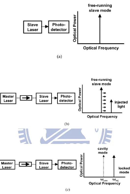
In 1980 Kobayashi and Kimura used GaAs lasers to demonstrate the injection locking experimental results. [1] Using two devices with close wavelength is necessary. In 2005 Lukas Chrostowski, Xiaoxue Zhao and Connnie J Chang-Hasnain used 1.55μm VCSEL to demonstrate the resonance frequency enhanced from 7GHz up to ~50GHz [2]. The technique is that one laser the master laser (ML) is external light source to inject photons in another laser the slave laser (SL). The resonant frequency enhancement might result from the external light injecting into the slave laser as a cavity increasing the photons in the slave laser. Using the technique has some advantages, such as side-mode suppression ratio(SMSR), enhancement of the relaxation oscillation, improvement of the nonlinear characteristic and chip frequency and so forth. It makes direct modulation more adequate for many applications.

The direct modulation of semiconductor lasers can be used for transmitting subcarrier-multiplexed signals at low cost of using injection locking to improve the nonlinear characteristic.[3] The resonance frequency enhancement by using the injection locking technique means that we will have much larger bandwidth can be used in optical communication. The technique can adequately improve the dynamic operation characteristic so that injection-locked lasers is a practicable way to use for future networks.

2.2 Theoretical Model

The dynamics of injection-locked lasers are simulated by rate equations which couple the temporal variations of the amplitude, the phase and the number of carriers of the slave laser:

)

(

cos

)

(

]

)

(

[

2

1

)

(

t

A

t

A

N

t

N

g

dt

t

dA

inj th











f

t

t

A

A

N

t

N

g

dt

t

d

inj th





















2

)

(

sin

)

(

]

)

(

[

2

)

(

)

(

]}

)

(

[

{

)

(

)

(

2

t

A

N

t

N

g

t

N

J

dt

t

dN

th p N















where A(t) is the field amplitude, defined as A2 (t)=S(t), where S(t) is the photon

number.φ (t) is the phase difference between the temporal laser field of the slave laser and master laser. N(t) is the carrier number and J is the injection current. Nth is the

threshold carrier number, g is the linear gain coefficient, γ P is the photon decay rate,

κ (= 1/τ in ) is coupling coefficient, τ in is the cavity round-trip time of the slave laser,

α is the linewidth enhancement factor of the slave laser, and γN is the carrier decay

rate. N th also defines the carrier number at the onset of lasing, and contains both

transparency carrier number and photon loss rate: gN =N tr+γ p/g .

By applying small signal linear approximation and stability analysis to the above rate equations [4, 5, 6], the injection locking range, ΔωL ,and locking stabilities

can be derived and plotted as following:

)

(

)

(

1

0 0 2

A

A

A

A

_inj L inj



















Eq 2.2.1 Eq 2.2.2 Eq 2.2.3 Eq 2.2.4

,where A 0 is the stationary amplitude of the slave laser under optical injection.

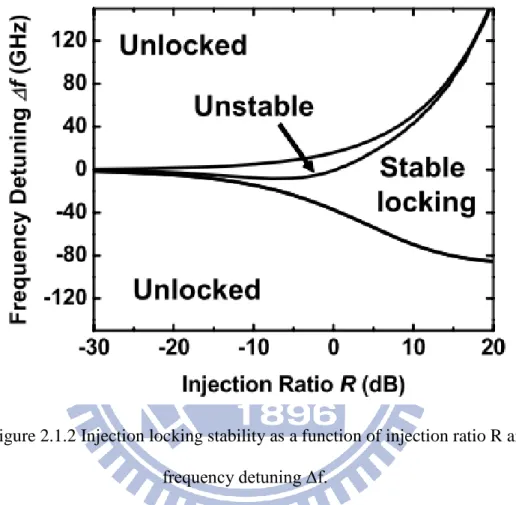
The regions of injection locking stability are shown as a function of injection locking parameters in Figure 2.1.2. Equation 2.2.4 and Figure 2.1.2 illustrate that stronger optical injection broadens the stable injection locking range.

Figure 2.1.2 Injection locking stability as a function of injection ratio R and frequency detuning Δf.

2.3 Linewidth enhancement factor

In 1981, Fleming and Mooradian demonstrated the linewidth of a semiconductor laser and found the linewidth is different from Schawlow-Townes predicted. They were unable to explain the result [7]. In 1982, Charles H. Henry wrote a paper about the theory of the linewidth of semiconductor [8]. In general, the phase of the optical field fluctuation to influence the laser linewidth. The fluctuations are due to the spontaneous emission.Linewidth enhancement factor(α) is the deviation of the imaginary part and real part of the refraction index.

n n n i r i r

n

n

n

    









Linewidth enhancement factor is attributed to the change in refractive index with carrier density. Due to the Kramers-Kronig relations, we can find the change in the imaginary part of the susceptibility will change the real part of the susceptibility.

The refractive:

i

r

jn

n

n





The value of the linewidth enhancement factor is dependent on the dimension of the quantization. The complex refractive index changes by the carrier density. We can observer from the follower formulas [9].

ch E E f f g ch r

R

dE

n

n

in ch ch v c ch



   







2 2 _{( )} ) ( ) )( ( 2 0

2

1

)

(

  





_   ch E f f g ch i

R

dE

n

n

in ch in v c ch



  







2 2 _{( )} ) ( / ) ( 2 0

2

1

)

(

   





_  

The change of the linewidth enhancement factor with different quantization dimension alters the term of g

ch. gch is the density-of-states of the electron-hole pair. It

is expresses by the step and delta functions, for a quantum well and quantum box. The change in the imaginary part of the susceptibility (gain or loss) will be influence by a corresponding change in its real part (refractive index) through the Kramers-Kronig relations. A symmetrical gain curve will lead to the dispersion curve of the refractive index has a zero at the frequency corresponding to the gain peak[10]. Large value will result in chirp under direct modulation in optical fiber communication.There are several methods to measure the linewidth enhancement factor, such as RF-modulation measurement, the interferometric measurement, the amplified spontaneous emission (ASE) method and using the locking region measurement [11]

2.4 Simulation theory

We start with a wave-guiding structure and define the z-direction when the direction of propagation. The basic equation is the Maxwell equations. However, we would like to go further and obtain a set of equations directly usable in solving the system. Under the assumption of the scalar wave, the wave equation can be solved with the variable separation technique.We assume that the solution to the wave equation can be written as the product

)

,

(

)

(

)

,

,

(

x

y

z

E

z

₀

x

y

E

_



_



where



is the optical frequency and

z

is the direction of the waveguide. The distribution



₀(x,y) can be calculated effectively by other approaches for instance the effective index method or the beam propagation method.The simulation software solves the problem including all the governing semiconductor equations. The

-dependent part of the electric field satisfies the equation.

)

(

)

(

)]

(

[

₂ 2 2

z

f

z

E

z

k

z













where f_(z) is the Langevin noise function because of spontaneous emission. We notice that the noise function is very important for a laser device because it is a driving force for the solution. For an isolated semiconductor laser, the physical solution for Eq. 2-1.2 would be zero if the spontaneous noise term was absent. A simple physical explanation is that the spontaneous emission noise generates or excites the photons, amplified by the the optical gain. The optical power is determined both by the spontaneous emission and the optical gain at any bias condition. The complex propagation constant k(z) contains information about the solution of the transverse and lateral dimensions, or in other words, it is calculated from the effective

Eq.2-1.1

index at a specific cross section in the xy-plane. The effective index and the k(z) are dependent on the frequency, material properties and the photon density ,as a result of the non-linear gain suppression.

Using Green's function in the analysis of DFB lasers was first proposed by C.H. Henry [12] and later extensively used by Tromborg [13] in deriving analytical formulas for DFB lasers. We has used the Green's function method because of its accuracy in treating spontaneous emission,and its conceptual simplicity.It is also suitable for numerical implementation.The Green's function method starts with the wave equation, 2-1.2. The objective is to obtain a compact expression for the solution to the noise driven wave equation. In the Green's functions method, the solution to Eq. 2-1.3 can be written as

W

dz

z

f

z

z

g

z

E

l





0

(

,

'

)

(

'

)

'

)

(

 

where f_(z') is the local Langevin force,

g

( z

z

,

'

)

the Green's function, and W the Wronskian of the wave equation. The integration is over the diode cavity length . The Wronskian W is a functional of the distribution of the wavenumber [k(w,N(z))] in general. The interpretation of Eq.2-1.3 is very simple according to the basic principle of the Green's function method. The Green's function method says that for any linear differential equation with a driving source term, the solution can be found by decomposing the source into many smaller pieces in space. The Green's function can be written as

)

'

(

)

(

)

'

(

)

'

(

)

'

(

)

(

)

'

,

(

z

z

Z

z

Z

z

z

z

Z

z

Z

z

z

z

g



_R



_L









_R



_L







Here



(z

)

is the Heaviside step function.

Z

L

(z

)

is the solution to the

homogeneous wave equation, which satisfies the boundary condition at the left laser

Eq.2-1.3

facet and internal interfaces for multi-section lasers but may not satisfy the boundary condition at the right laser facet. Z_R(z) is the corresponding solution which satisfies

the boundary condition at the right facet and the internal interfaces. The Wronskian can be written as

)

(

)

(

)

(

)

(

Z

z

dz

d

z

Z

z

Z

dz

d

z

Z

W



_{L R}



_{R L}

Since Z_L(z)and Z_R(z)are solutions to the homogeneous wave equation, it follows

from simple algebra that



0

dz

dw

in each waveguide section. This means that W is

position independent.Therefore, under a particular bias condition, the Wronskian is only a function of the frequency or wavelength.

For the detailed 2D E-field distribution, we need to use a more elaborated way to simulate this problem.The basic equations used to describe the semiconductor device behavior are Poisson’s equation and the current continuity equations from Maxwell’s equations for electrons and holes:

, where V is electrical potential, n and p are electron concentration and hole concentration, ND and NA are doping of shallow donors(D) and shallow

acceptors(A),fD and fA are occupancy of donor (D) and acceptor(A) levels, Ntj is

density of j th deep trap,ftj is occupancy of the j th deep trap level , Jn and Jp are

current flux densities,Rntj and Rptj are electron and hole recombination rate for

Eq.2-1.7 Eq.2-1.6

Eq.2-1.8 Eq.2-1.5

quantum well, Rsp is spontaneous recombination rate, Rst is stimulated

recombination rate, Rau is auger recombination rate. By solving the above equation

sets, we could calculate more precisely the field distribution within the cavity.

2.5 Couple-Wave Equations

As was discussed in the previous section, the problem has been reduced to solving for the Green's function and the corresponding Wronskian. These in turn require the knowledge of the solution of the homogeneous wave equation

0

)

(

)]

(

[

₂ 2 2









z

E

z

k

z



where k(z) is the wavenumber of the waveguide given by

2 0 2 2 2

c

n

k





0

c is the speed of light in vacuum and n is the refractive index. The wave number may depend directly on z due to the grating structure or variation in the material composition and indirectly through the carrier density and photon density variations along the waveguide.

In DFB and DBR lasers, corrugations are made along the wave guides which introduce coupling between forward and backward waves. The purpose is to perturb the propagation constant k (z) to achieve desirable scattering effects to the

propagating waves. In a laser with a grating of period Lg, its effective refractive

index can be written as

)

)

(

2

cos(

)

(

2

~











z

z

L

n

n

n

g



Eq2-2.1 Eq2-2.2 Eq 2-2.3

where we consider the general case that the grating period may vary as a function of position. denotes the slow varying part of the complex index and 2 n( ) is the magnitude of the index variation which is again a complex quantity. We define a reference wave number which is usually set to the Bragg wave number in simple grating structures at threshold condition such that







g

L





0

where

 

used to denote the average grating period.



₀is a constant independent of the frequency and injection conditions. In general, we can assume that the change in the grating period is smooth and write the following expansion,

) ( 0 z L_g





ch



   

where 



ch(z)is caused by some form of chirp grating variation of grating period.

Based on Eq. 2-2.3, we re-write the wave number as

]

]

)

(

2

cos[

2

₀ ~ 0

















k

z

j

k









_ch         

_









_k

_e

2j( ch)z] j

_e

2j( ch)z] j ~ 0 0 0    

_





where 0 0 ~ ~   _   c n k and 0 c n





 Eq 2-2.4 Eq 2-2.5 Eq 2-2.7 Eq 2-2.6 Eq 2-2.8 Eq 2-2.9

Since only the optical frequencies close to the Bragg condition are considered, the second term in Eq. 2-2.7 is small compared with



0. Similarly we assume that the

coupling coefficient is much smaller than



₀. In the following derivation, we will neglect higher order terms of and . We propose a trial solution of the form: z j z j z

R

z

e

L

z

e

E



₍

₎

 0



₍

₎

0

where L(z)and R(z)are used to denote the slow varying amplitudes of waves going left and right, respectively. We substitute it into the wave equation to get the following algebra:

0

)

)

(

)

(

(

)

(

)

(

]

)

(

)

[(

2

]

)

(

)

(

[

0 0 0 2 2 0 2 2 0 0 0 0 ) ( ) ( ) ( ) ( 0 2 0



















            z j z j z j z z L z j z z R z j z z L z j z z R z j z j

e

z

L

e

z

R

k

e

e

e

e

j

e

z

L

e

z

R

       

_



Treating and as small quantities, we expand the wave number as follows.

)

(

2

2 ( ) ] 2 ( ) ] ~ 2 0 2









j ₀ _ch z j



 j ₀ _ch z j

e

e

k

k







 



 

+higher order terms.

which is then substituted into Eq. 2-2.11. To simplify the notation, we introduce a slow varying function











_g

(

z

)

2



_ch

(

z

)

z

We further assume that the wave amplitude is a slow varying function of z and

neglect the second derivatives involving

(

₂

(

)

)

2

z

z

R





and

(

₂

(

)

)

2

z

z

L





.After the terms

involving



₀2 are canceled, we are left with the following equation.

Eq 2-2.10

Eq 2-2.11

Eq 2-2.12

0

)

)

(

)

(

)(

(

2

]

)

(

)

[(

2

0 0 0 0 0 2 2 0 2 2 2 2 ~ 0 ) ( ) ( 0

















           z j z j j z j j z j z j z z L z j z z R

e

z

L

e

z

R

e

e

k

e

e

j

g g      









Since R(z) and L(z) are independent functions, this equation makes sense only when terms with the same propagation factor sum up to zero. In other words, the terms with

_e

j0Z

and

_e

j0Z

must sum up zero, respectively. Collecting these terms, we find

0

)

(

2

)

(

2

)

(

2

0 ~ 0 ) ( 0











   

z

L

e

z

R

k

j



R_zz







j gz

0

)

(

2

)

(

2

)

(

2

₀ ~ 0 ) ( 0









  

z

R

e

z

L

k

j

j z z z L







g



or in matrix notation:























































  

)

(

)

(

)

(

)

(

)

(

)

(

~ ~

z

L

z

R

k

j

e

j

e

j

k

j

z

L

z

R

z

g g j j





Eq 2-2.14 Eq 2-2.15 Eq 2-2.16

2.6 Theory of relative intensity noise(RIN)

RIN peak is a good show of the relaxation frequency of the device. The driving force not input current is the Langevin force (F

s, Fn and Fφ) of the field due to the

spontaneous emission. The Langevin force is assumed to be irrelative white Gaussian noise [14]. The relative intensity noise (RIN) spectrum is frequency dependence. The former can be derived from the rate equations.

The intrinsic relative intensity noise(RIN) of a device is defined as

P

t

P

RIN

2

0

)

(

2









P

0 is the average power and δP(t) 2

is the mean square power fluctuation. From a small-signal analysis of the rate equations for a single-mode laser, we can derive the noise spectrum of the device. The relative intensity noise spectrum of external light injected locked device can be derived using the follow rate equations [15].

Eq 2-3.1 s sp inj inj c p

F

R

t

S

S

k

S

S

s

N

N

G

dt

ds

th























2

cos(

(

)

)

1

) ( 0





















F

R

t

S

S

k

f

N

N

G

dt

d

sp inj inj c th























2

sin(

(

)

)

2

) ( 0 N s

F

S

s

N

N

G

N

q

I

dt

dN

th



















1

) ( 0 Eq 2-3.2

S ,  and N are the photon number, the phase and the carrier number inside the slave laser cavity. G0 is the gain coefficient, N0 is the transparency carrier number, τp

is the photon lifetime, τn is the carrier lifetime, I is the slave laser bias current, ε is the

gain compression factor, and α is the linewidth enhancement factor. Fs , Fφ and Fn are

the noise terms. Δω is the detuning between the master and slave laser. S is the _inj photons injection into the slave laser. k_c is the coupling coefficient, which determined by the photon injected into the cavity-round trip time.

We based model of injection-locked rate equation is usually used to describe the interaction between photons and carriers inside a laser cavity. When an additional light source is injected into the cavity, the system preserves the general form of the original equations, but with extra terms describing the effects of the injection.

t j t j t j t j t j N N t j t j s s

e

S

S

S

e

N

N

N

e

e

S

S

S

e

F

F

e

F

F

e

F

F

      





































        





















)

(

,

)

(

)

(

,

)

(

)

(

,

)

(

,

)

(

1 0 1 0 1 0 1 0

Substituting into the injection-locked rate equation

 

)

(

))

(

)

sin(

)

cos(

2

)

(

)

(

2

)

(

1

)

(

)

1

1

(

)

(

1

)

(

1 0 0 0 1 0 1 0 0 1 0 0 0 1 0 0 0 1





































 s inj inj inj inj c p t j tr

F

S

S

S

S

S

k

e

S

S

S

N

G

S

S

S

S

N

N

G

S

i





















































 Eq 2-3.3

For the phase part:

)

(

))

(

)

cos(

)

sin(

2

)

(

(

(

2

)

(

)

(

1 _{0 0 1} 0 1 0 1



























S

F

_

S

S

k

N

G

i











_c inj





_inj





_inj





Finally, for the carrier part:

 

( ) 1 ) ( ) 1 1 ( ) ( 1 ) ( ) ( 0 0 1 0 0 0 1 0 0 0 1 1 _            tr _n s t j F S S N G S S S S N N G e N N i                   

Equations (2-3.3), (2-3.4), (2-3.5) are written in matrix form:











































N s

F

F

F

N

S

A



_ 1 1 1                                                                        s tr inj inj c inj inj c inj inj c inj inj c p tr S S G i S S S N N G S S S k i S S k S S G S S k S S k S S S N N G i A                       1 1 0 ) 1 1 ( 1 ) ( 2 ) cos( ) sin( 2 1 ) sin( 2 ) cos( 1 ) 1 1 ( 1 ) ( 0 0 0 0 0 0 0 0 0 0 0 0 0 0 0 0 0 0 0 0 0 0 0 0 0

The laser RIN

)

(

)

(



S

₁



RIN



The small-signal modulation response can also be found from this system by considering I as the small signal modulation current.













































I

A

N

S

0

0

1 1 1 1



Eq 2-3.4 Eq 2-3.5

The modulation response transfer function will be

)

(

)

(

)

(

1







I

S

H



The light injected into the cavity of the slave laser and depletes the carrier density. It makes the spontaneous emission rate reduced and more photons are coupled in phase into the amplified injection field. The more photons in phase and the relaxation frequency should enhance. The RIN spectrum shows that the relaxation frequency peak becomes higher with injections. At a lower injection level directly adds photons into the slave laser cavity by using more carriers, compensating the gain saturation and enhances the relaxation peaks of the slave laser. Under the stronger injections condition, the injected photons deplete the most of the available carriers, saturate the signal and decrease the relaxation peaks finally. It prevents the further improvement of the relaxation frequency.

References

[1] S. Kobayashi and T. Kimura,"Coherence on injection phase-locked AlGaAs semiconductor laser," Electronics Letters, vol. 16, pp. 668-670, 1980

[2] Lukas Chrostowski, Xiaoxue Zhao and Connie J. Chang-Hasnain, “50 GHz Directly-Modulated Injection-Locked 1.55 μm VCSELs,” Optical Society of America, 2005

[3] Erwin K Lau,"High-Speed Modulation of Optical Injection-Locked Semiconductor Lasers," Electrical Engineering and Computer Sciences University of California at Berkeley, 2006

[4] S. Mohrdiek, H.Burkhard, and H. Walter, "Chirp reduction of directly modulated semiconductor lasers at 10 Gb/s by strong CW light injection," J. Lightw. Technol., vol. 12, no. 3, pp. 418-424, Mar. 1994.

[5] R. P. Braun, G. Grosskopf, R. Meschenmoser, D. Rohde, F. Schmidt, and G. Villino,"Microwave generation for bidirectional broadband mobile communications using optical sideband injection locking," Electron. Lett., vol. 33, no. 16, pp. 1395-1396, Jul. 1997.

[6] X. Lixin, W. H. Chung, L. Y. Chan, L. F. K. Lui, P. K. A. Wai, and H. Y. Tam, "Simultaneous all-optical waveform reshaping of two 10-Gb/s signals using a single injection-locked Fabry-Perot laser diode," IEEE Photon. Technol. Lett., vol. 16, no. 6, pp. 1537-1539, Jun. 2004.

[7] M. W. Fleming and A. Mooradian, “Fundamental line broadening of single-mode(GaA1)As diode lasers,’’ Appl. Phys. Lett., vol. 38, p. 511, 1981.

[8] CHARLES H. HENRY, “Theory of the Linewidth of Semiconductor Lasers,’’ IEEE journal of quantum electronics, vol. QE-18, no. 2, February 1982

Enhancement Factor α of Multidimensional Quantum Wells, “ Japanese journal of applied physics, vol 28 pp1280-1281, 1989

[10] MAREK OSINSKI and JENS BUUS, “Linewidth Broadening Factor in semiconductor Lasers-An Overview” Quantum Electronics, IEEE Journal of, 1987 [11] G. Liu, X. Jin, and S. L. Chuang,“Measurement of Linewidth Enhancement Factor of Semiconductor Lasers Using an Injection-Locking Technique” IEEE photonics technology letters, VOL. 13, NO. 5, MAY 2001

[12] C. H. Henry, ``Theory of spontaneous emission noise in open resonators and its application to lasers and optical amplifiers,'' J. Lightwave Technol., LT-4, 288-297 (1986).

[13] B. Tromborg, H. Olesen, and X. Pan, ``Theory of linewidth for multi-electrode laser diodes with spatially distributed noise sources,'' IEEE J. Quantum Electron., QE-27, 178-192 (1991).

[14] X. Jin and S. L. Chuang , “Relative intensity noise characteristics of injection-locked semiconductor lasers, “APPLIED PHYSICS LETTERS, vol 77, NUMBER 9 , 28 AUGUST (2000)

[15] Lukas Chrostowski, “Optical Injection Locking of Vertical Cavity Surface Emitting Lasers,” Fall (2003)

Chapter 3.

Simulation Result of the Self-pulsation Laser

3.1 Background on design

In this section a single gapped FP laser diode will be introduced which forms the basis for our platform.The single gap laser is fabricated by etching into the waveguide of the FP laser diode. The gaps act as reflection centers and produce a modulation of the reflection and transmission spectra dependent on the characteristics of the slot such as gap position, gap depth to which it is etched and slot width. Even if the gap is not etched into the active regions it will still interact with the mode of the electric field of the waveguide as the mode profile is not fully confined to the active region and will expand into the surrounding cladding regions. The 1D first order electric field mode profile modeled using the finite difference time domain technique for a simple laser structure with active region depth of 1 µm, upper cladding region of 1 µm and lower cladding of 1 µm with active region refractive index of 3.55 and cladding region refractive index 3.41, which are normal values for an InGaAsP active region sandwiched between InP cladding regions, are shown below in Fig. 3.1.1.

Figure. 3.1.1 Mode profile of the fundamental mode and refractive index profile through the laser structure.[1]

From Fig. 3.1.1 the fundamental mode is seen to penetrate into the cladding region so any perturbation in this area will influence the mode profile. The scattering matrix method is a easy and accurate technique which can be used to determine the reflection and transmission from gaps etched into the laser cavity.Numerous texts deal with the SMM of which is a good introduction.Of particular importance in a laser structure is the ability to determine loss using the method. This is an important advantage of the SMM over that transmission matrix method (TMM). A FP laser with one etched slot can be described as three cavities with different interface reflections and transmissions as described below in Fig 3.1.2.

Figure 3.1.2. Schematic description of single slot laser diode.[1]

In fig. 3.1.2, ni refers to the effective refractive index in these section of the laser

structure, while ri refers to the reflection from the interfaces as shown above. Each

section can be described as a separated cavity and the total reflection and transmission is then found.The back section amplitude reflection from the left side and right side is described as

 

 

                 b b b b bl L i L i

r

r

t

r

t

r

r

~ 1 2 ~ 1 1 1 1 2 exp 1 2 exp   and

 

 

 

                   b b b b br L i L i

r

r

t

r

t

r

r

~ 1 2 ~ 2 1 2 2 2 exp 1 2 exp  

respectively where β is the complex propagation constant ( β= βre + iβim ) and Lb is

the back section cavity length. The back section amplitude transmission from the left side is described as

 

               b b b b bl L i L i

r

r

t

t

t

~ 1 2 ~ 2 1 2 exp 1 exp   and

t

t

br bl

giving a power reflection and transmission is Rbl = rbl2 and Tbr = tbr2 respectively. The

reflection and transmission of the back section and gap region is found by including the back section reflection and transmission in the SMM calculation as follows

 

 

                  s s bl s s bl sl bl L i L i

r

r

t

r

t

r

r

~ 3 ~ 3 3 3 2 exp 1 2 exp   and

 

                s s bl b b bl sl bl L i L i

r

r

t

t

t

~ 3 ~ 3 2 exp 1 exp  

again by a continuation of this method the reflection and transmission amplitudes for the full laser structure can be determined as

 

 

                   f f sl bl f f sl bl total L i L i

r

r

t

r

t

r

r

~ 4 ~ 4 4 4 2 exp 1 2 exp   and

 

                 f f sl bl f f sl bl total L i L i

r

r

t

t

t

~ 4 ~ 4 2 exp 1 exp  

where the reflection and transmission from the right is found in a similar fashion to the total from the left.The calculated power reflection using an experimentally determined gain profile is shown in Fig. 3.1.3 [1]

Figure 3.1.3 Calculated reflection spectrum of a single gap laser (1550 nm).

3.2 Wave intensity distribution analysis

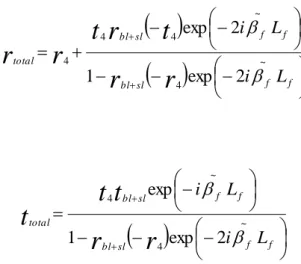
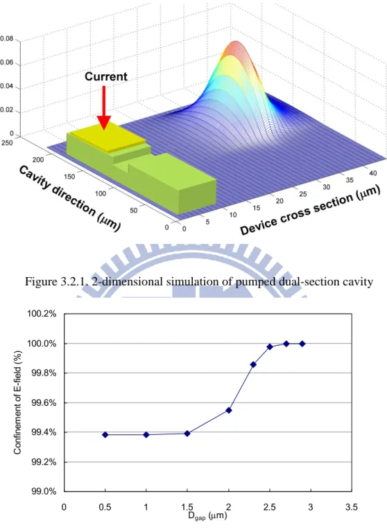
To solve this problem, initially we took an finite difference technique [4] for the start. The variation in the third dimension is assumed to be uniform for now. When we simulate the device structure, the pumped region was indexed a little higher to mimic the optical source field. Fig. 3.2.1 shows the two dimensional field distribution. When calculating the axial field intensity, we can find out a sharp increase of confinement when the Dgap increases more than 2um as shown in Fig. 3.2.2.

For the detailed 2D E-field distribution, we need to use a more elaborated way to simulate this problem.The basic equations used to describe the semiconductor device behavior are Poisson’s equation and the current continuity equations from Maxwell’s equations for electrons and holes:

, where V is electrical potential, n and p are electron concentration and hole concentration, ND and NA are doping of shallow donors(D) and shallow

acceptors(A),fD and fA are occupancy of donor (D) and acceptor(A) levels, Ntj is

density of j th deep trap,ftj is occupancy of the j th deep trap level , Jn and Jp are

current flux densities,Rntj and Rptj are electron and hole recombination rate for

quantum well, Rsp is spontaneous recombination rate, Rst is stimulated recombination

Figure 3.2.1. 2-dimensional simulation of pumped dual-section cavity

Figure 3.2.2. Calculation of confinement of E-field in the quantum well axial direction. 99.0% 99.2% 99.4% 99.6% 99.8% 100.0% 100.2% 0 0.5 1 1.5 2 2.5 3 3.5 Dgap (m) C on fin em en t o f E-f ie ld (% )

Figure 3.2.3. (a) Field distribution: Wgap=5μm, but with no air gap; (b) Field

distribution on Wgap=5μm,Dgap=5 μm

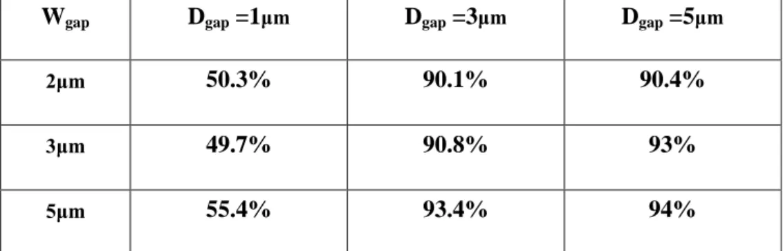
Wgap Dgap =1μm Dgap =3μm Dgap =5μm

2μm 50.3% 90.1% 90.4%

3μm 49.7% 90.8% 93%

5μm 55.4% 93.4% 94%

By solving the above equation sets, we could calculate more precisely the field distribution within the cavity. First of all, we started the simulation under R1=R2=0.32

and I2 off .We focus now on the wave intensity distribution with an air gap of

different depths and widths.Figure 3.2.3(a) shows the E-field distribution without any gap. Figure 3.2.3(b) shows that the wave intensity is re-distributed when the depth of the air gap is increased to 5μm, the field is hardly penetrated into the right section. We calculated the wave intensity distribution ratio of the pumped cavity versus the overall field intensity shown at the Table 1. When there is no depth on the chip, the left field intensity is about 50.3% at width of gap is 2μm and is 55.4% at the width of the air gap is 5μm. There is little difference of intensity ratio between the two cases. However, once we start increase Dgap, and widen Wgap, the obvious partition of field intensity can be observed. The detailed 2 dimensional calculation is summarized in table 1. As we could see, the influences of the air gap is profound. Most of the excited E-field is confined in the pumped region, however, some of them will leak into the other un-pumped (or cold) cavity. This leakage is the source of interference of the other section of laser and usually we don’t know, to what extent, this leakage will disturbing the operation of the other laser unless we can quantify it. Using this method, we can estimate the possible feedback or coupling between multiple sections of semiconductor lasers.

3.3 Two-Section Laser dynamic characteristics with

different slot depth

3.3.1 L-I curve

When we put a air slot in the middle section of the two-section laser, the basic performances such as laser power, current distribution or leakage current , which could be influenced to what extent by different Dgap.Therefore,we have to do some

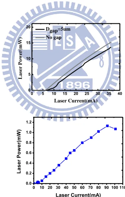
simulation and measurement about the basic performances after the focus ion beams process. 0 5 10 15 20 25 30 35 40 0 5 10 15 20 L a se r P o w e r (m W ) Laser Current(mA) Dgap=5um No gap

Figure 3.3.1.L-I curve (a) simulation results with air gap Dgap=5um and with no gap(b)

measurement result with Dgap=5um

0 10 20 30 40 50 60 70 80 90 100 110 0.0 0.2 0.4 0.6 0.8 1.0 1.2 L a s e r P o w e r( m W ) Laser Current(mA)

The figure 3.3.1(a) shows the L-I simulation result of un-FIB laser, which is normal average performance on the two-section laser. The figure 3.3.1(b) shows the L-I measurement result under different bias current. In addition, the threshold current is matches, while the power is decrease at 91mA due to large bias current which leads to the spatial hole burning.

If we etch the laser to Dgap=5um,the threshold current could increase and the

laser power decrease a little. Hower,etching to the active layer, we can see not only the threshold current will increase more but also the laser power will fall down sharply. We could have the most moderate Dgap to etch the two section laser.

3.3.2 Leakage current

Our monolithic two-section laser is not composed of two independent lasers.However,the two sections have a common laser grating and an optical cavity originally. After the FIB etching process, the monolithic laser has two asymmetric laser cavities, but it still have common active layers.So,the other characteristic what we want to know is the laser current distribution after FIB process.

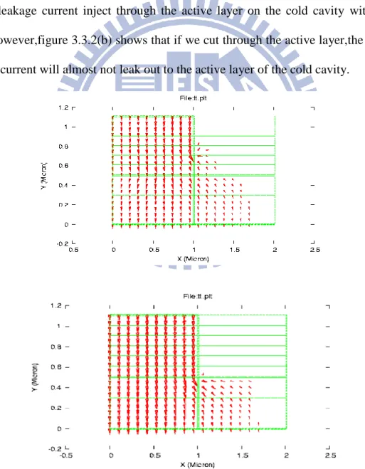
Because the pumped cavity current could leak through the cold cavity, it might give rise to some influence on cold cavity. From the figure 3.3.2(a), we can see that some leakage current inject through the active layer on the cold cavity with an air gap.However,figure 3.3.2(b) shows that if we cut through the active layer,the pumped cavity current will almost not leak out to the active layer of the cold cavity.