基於光刺激發光技術用於Al2O3:C材料之劑量消光研究

(1)

國立交通大學

電子物理研究所

碩士論文

基於光刺激發光技術用於 Al

₂

O

3

:C 材料之劑量消光研究

Optical Bleach For Dosimetry in Al

₂

O

₃

:C Base On

Optically Stimulated Luminescence Technique

研究生：李勁吾

指導教授：謝奇文博士

(2)

基於光刺激發光技術用於 Al

2

O

3

:C 材料之劑量消光研究

Optical Bleach For Dosimetry in Al

2

O

3

:C Base On Optically Stimulated

Luminescence Technique

研究生：李勁吾 Student：Jing-Wu Li

指導教授：謝奇文教授 Advisor：Prof. Chi-Wen Hsieh

國立交通大學

電子物理所

碩士論文

A Thesis

Submitted to Department of Electrophysics College of Science

National Chiao Tung University in Partial Fulfillment of the Requirement

for the Degree of Master

in Electrophysics

July 2009

(3)

基於光刺激發光技術用於 Al

₂

O

3

:C 材料之劑量消光研究

學生：李勁吾指導教授：謝奇文教授

國立交通大學電子物理所碩士班

摘要

為了解決 Al

2

O

3

:C 材料在同一光激發螢光強度下對應兩個高低不同的

輻射劑量值問題，本文嘗試使用部分光清除方法，得到在相同照射時間下

光激發螢光強度有不同的下降速率，於是高低兩個值分開。

實驗上利用可見光和紫外光作為光清除燈源，發現紫外光有清除能力

但也有累積劑量的效果。

理論上利用了能帶理論模擬電子在 Al

2

O

3

:C 材料中的光清除行為，和最

大光清除效果。模擬結果和實驗值比對，進而以此數學模型預測激發光源

調變後材料 Al

2

O

3

:C 的發光行為變化。

(4)

Optical Bleach For Dosimetry in Al

₂

O

₃

:C Base On Optically

Stimulated Luminescence Technique

Student：Jing-Wu Li Advisor：Prof. Chi-Wen Hsieh

Department of Electrophysics

National Chiao Tung University

Abstract

An optical bleach system was designed to deal with a puzzle where one of OSL intensity in Al2O3:C indicating two different amounts of doses. After the optical bleach,

a different OSL decay speed was discovered to separate those two doses. This research helps in the emergency management of nuclear accident or high radiation exposure event.

Experimentally, visible light and ultraviolet light was used as the bleach light source. UV was discovered with anti-bleach property. Therefore, a flexible UV thin film filter was set in the visible light bleach system.

Furthermore, a dynamic band theorem simulation was used to describe electron property inside the Al2O3:C. Optical bleach simulation and maximum bleach

simulation match the experimental data successfully. The model can not only predict the optical bleach effect but also the OSL signal variance by changing excitation photon energy.

(5)

誌謝

(Acknowledgement) 在交大風雨璀璨的兩年即將要進入尾聲，回首過去所經歷一切的人、事、物，是無比的可貴和難忘。感恩謝奇文老師一年前不嫌棄的承接，我可能現在還在交大篳路藍縷、四處流浪，而不是以喜孜孜的心情寫此篇致謝辭。與謝老師一同做研究的日子裡，學到的不只是做研究的方法和精神，還有老師對於學生的生命關懷，進而成為亦師亦友的夥伴關係，老師不但沒有絲毫的架子，反而像家人、像兄長一樣，無微不至的照顧。甚至老師個人的有形、無形的資產都能共同一起分享，讓學生感受到無比的溫馨。感恩老師的用心，給予學生許多的學習資源和機會；感恩老師的付出，讓學生得以健全的學習和成長；也感恩謝老師的耐心指導，讓本篇論文得以順利完成。感謝幽默風趣、和藹可親的陳坤焙老師在實驗上的大力支持和協助，讓學生從不會的新手漸入佳境。感恩老師的不吝付出，感恩老師巨細靡遺的建議與叮嚀。感謝師尊鐘太郎老師和羅志偉老師對論文的指導與督促，使之趨於完善。感恩實驗室景元學長、清大電機819實驗室的同儕： Nash、 TD、Ker Ker、豹哥。在我苦悶做研究的時候增加了不少團康樂趣，成為我進去實驗室的動力，使我順利完成工作。

再次感恩所有曾幫助過我的老師、摯友，讓我可以順利的邁向另一個新的旅程，畢生難忘。

(6)

List of Figures

Figure 1-1 Illustrate operation principle of OSL & TL 2 Figure 1-2 Illustrate electron behavior by band diagram. 3 Figure 1-3 Schematic of OSL & TL physical property 4 Figure 1-4 Dose Fractionation of OSL technique in 25 times measurement 5 Figure 1-5 Stable signal of OSL technique for 120 days store 6 Figure 1-6 Schematic picture for real-time radiation therapy by OSL

technique

10

Figure 1-7 Demonstration of confusion in dose dependence of Al2O3:C with

same OSL signal.

12

Figure 2-1 Band diagram 13

Figure 2-2 Schematic one-trap, one recombination-center model 14 Figure 2-3 Schematic multi-trap, multi-recombination-center energy band

diagram

16

Figure 2-4 R. Chen’s simulation compare with experimental data 17 Figure 2-5 Schematic representation of the three main OSL stimulation

modes, CW-OSL, LM-OSL and POSL.

18

Figure 2-6 OSL result under three different stimulated modulation 19 Figure 2-7 Illustrate timing control of POSL system. 21

Figure 2-8 Schematic of Al2O3 structure. 22

Figure 2-9 Optical property of Al2O3:C 22

Figure 2-10 LuxelTM_{OSL Badge of alpha-Al}

2O3:C 23

Figure 2-11 Landauer OSL dosimeter 24

(9)

Figure 2-13 Illustrate mechanism for Luxel Badge in reading process. 26 Figure 2-14 The GUI face of Landauer Automatic 200 POSL Reader. 26

Figure 2-15 Ultraviolet System 27

Figure 2-16 The emission spectrum of UVA light tube. 27 Figure 2-17 Experimental setup for visible light bleach. 28 Figure 2-18 The emission spectrum of visible light source. 28 Figure 2-19 The transmission property of UV filters. 29 Figure 3-1 Flow chart for Landauer OSL reader reliability test. 30 Figure 3-2 Average distribution of 1, 5, 10, 50, 100Gy for 40 Times OSL

Read out.

31

Figure 3-3 Standard deviation of four elements in background and 1Gy Badge.

31

Figure 3-4 Standard deviation of four element in 5Gy and 10Gy Badge. 31 Figure 3-5 40 times readout distribution and standard deviation of four

element in three 50Gy Badges.

32

Figure 3-6 40 times readout distribution of 5Gy & 10Gy. 33 Figure 3-7 40 times readout distribution and standard deviation of four

elements in three 100Gy Badges.

33

Figure 3-8 Visible Light Bleach effect for 5~100Gy Badge 34 Figure 3-9 The Visible light Bleach effect for Element 1, 2, 3 and 4. 35 Figure 3-10 UV light pumping effect for background dose badge. 36 Figure 3-11 UV light bleach effect for 1~10 Gy badge. 36 Figure 4-1 The flow chart of simulation process. 37 Figure 4-2 The steps of ordinary differential equation in Matlab 2007

software.

(10)

Figure 4-3 Schematic R. Chen’s multi-trap, multi-recombination-center energy model.

38

Figure 4-4 Repeat R. Chen’s simulation result. 41 Figure 4-5 F-center conversion simulation result and experimental data. 43 Figure 4-6 Optical bleach simulation result with experimental data. 43 Figure 4-7 Simulation matches the OSL decay speed with different dose. 44 Figure 4-8 Detail bleach effect of optical bleach effect in 1~ 10Gy with

simulation result.

44

Figure 4-9 Bleach effect with UV filter in the visible light system. 45 Figure 4-10 Visible Light bleach without UV filters. 46 Figure 4-11 Different light source has different saturation point 47 Figure 4-12 Bleach effect will achieve to a saturation point. 47 Figure 4-13 Two trap stimulated competition band diagram. 48 Figure 4-14 OSL Intensity for two trap stimulate competition. 49 Figure 5-1 The proposed flowchart to distinguish the over dose and under

safety margin situation.

50

Figure 5-2 Schematic diagram of prototype design for UV-light-source OSL reader.

(11)

List of Tables

Table 1-1 The comparison table of RFL and OSL 5

Table 1-2 Standard dose calculation 8

Table 2-1 The function of four chip in OSL badge 23

Table 2-2 Luxel badges with standard dose 23

Table 4-1 Calculation of lowest common multiple for bleaching photon 46

(12)

1.1 Background

Chapter 1 Introduction

1.1 Background

Radiation detection and radiation image are both well-known technologies in nowadays. X-ray, CT, PET, and MRI are powerful instruments for medical diagnosis. Generally, radiation image (detection) principle can be divided into two ways. One is detecting the radiation signal which goes through human body directly or reflection from human body. The other way is putting radioactive isotopes into human body as bio-marker, then detect the radiation signal coming from human body. This method needs more radiation dose to construct bio-image or radiation image.

Personnel radiation detection is one of the radiation detection applications. It is used to protect people who have been exposed in high energy environment. Traditionally, personnel radiation detection was mainly used Thermo-luminescence (TL) technique to evaluate radiation dose that people have been absorbed. Because TL signal is proportional to the dose of ionizing radiation, dose absorption can be taken from inverse calculation by TL signal. However, due to many of restrictions come from TL technique. Japanese developed Radio-Photo-Luminescence (RPL) technique to overcome TL drawback. Meanwhile, American developed a similar technique which is called “Optically Stimulated Luminescence (OSL)” in personnel Dosimetry [1].

In Taiwan, the OSL technique was introduced by Dr. K. B. Chen of National

Tsing-Hua University in 2007. This study tries to realize the intrinsic physical behavior of OSL material and makes the preliminary work to design more applications especially in personnel dosimetry study based on OSL technique.

(13)

1.2 OSL vs. TL

Optically Stimulated Luminescence (OSL) is the luminescence, which is emitted from material during light exposure. Thermo-Luminescence (TL) is the luminescence, which is emitted from material during heat exposure. OSL using photon as excitation energy and TL using heat as excitation energy are shown in the Fig.1-1.

Fig. 1-1. Illustration of operation principle of OSL & TL (a) Optical Stimulated Luminescence (b) Thermal-Luminescence [2].

Basically, the luminescence of TL and OSL is the photon emitting process of electron-hole pair recombination. The electrons in the valance band receiving a high energy radiation will be pumped into the conduction band and then relax to a meta-stable state. The trapped electrons in meta-stable state could be thermal stimulated or optical stimulated to the conduction band and then fell down to lower energy state (recombination center) to produce Luminescence. Fig.1-2 and Fig.1-3 shows the illustration of this physical property.

Thermal Stimulation

(14)

1.2 OSL vs. TL

Conduction Band Valence Band Conduction Band Valence Band Conduction Band Valence Band Conduction Band Valence Band (a) (b) (d) (c) Recombination Center Electron Trap Center

Fig.1-2. Illustration of electron behavior in band diagram. (a) Receiving a high energy radiation. (b) Relaxing to meta-stable states (c) Optical stimulated or thermal stimulated (d) Emit photo by electron-hole pair recombination.

However, there are some disadvantages of TL technique. Since that TL read out needs a stable heat source to access the photons, the property makes TL device difficult to minimize the size and sense the photons in real-time mode. Besides, TL is an environmental sensitivity that TL signal will often be disturbed by environmental temperature. And heating process is a global effect; the whole TL badge will lose the energy level mark when it has done the read out. This means we cannot recover the dosimetry.

(15)

1.2 OSL vs. TL

Fig. 1-3. Schematic physical property of OSL & TL. (A) Before irradiation (stable state) (B) After irradiation (meta-stable state) (C) Optical stimulated or heat stimulated (D) Back to stable state [1].

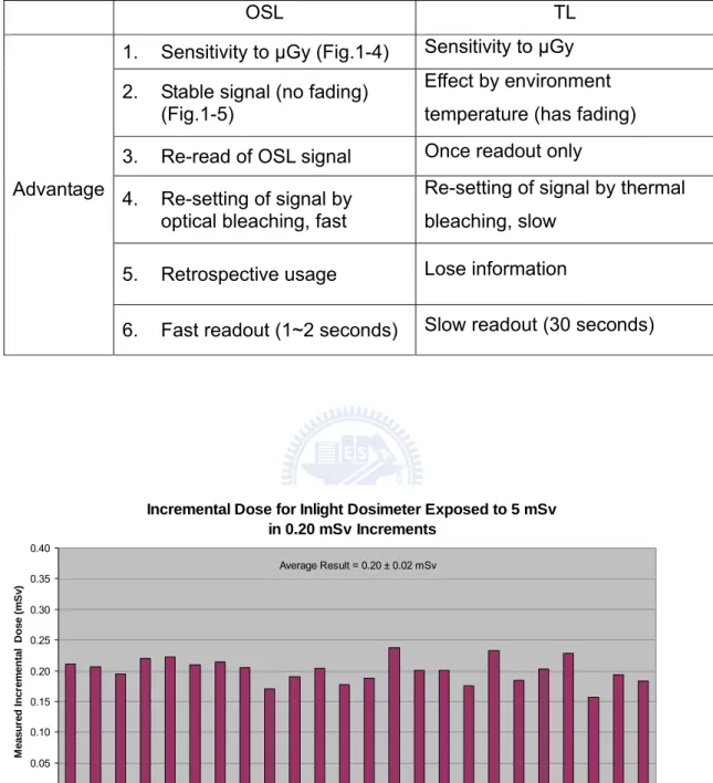
Clearly, to integrate the optical fiber with OSL technique could make the radiation dose monitoring on-line possible in clinics [3]. In addition, OSL has another advantage that is the retrospective usage of the badge. Since the depletion rate of each stimulated process (readout stage) with pulsed laser triggering only consumes a few of electron concentration in meta-stable state, and there are still some concentrations of meta-stable state survived. It can not only re-read dose information in the OSL badge but also detect low dose absorption precisely [2]. The property means the OSL is more sensitive compared with TL material and what makes the reproducible readout process possible. An OSL and TL comparison is shown in the Table 1-1.

(16)

1.2 OSL vs. TL

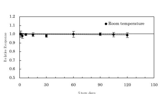
Incremental Dose for Inlight Dosimeter Exposed to 5 mSv in 0.20 mSv Increments 0.00 0.05 0.10 0.15 0.20 0.25 0.30 0.35 0.40 1 2 3 4 5 6 7 8 9 10 11 12 13 14 15 16 17 18 19 20 21 22 23 24

Dose Increment Number

M easu red I n cr emen tal D o se (m S v ) Average Result = 0.20 ± 0.02 mSv

Table 1-1. The characteristics comparison of TL and OSL

OSL TL

1. Sensitivity to μGy (Fig.1-4) Sensitivity to μGy 2. Stable signal (no fading)

(Fig.1-5)

Effect by environment temperature (has fading) 3. Re-read of OSL signal Once readout only 4. Re-setting of signal by

optical bleaching, fast

Re-setting of signal by thermal bleaching, slow

5. Retrospective usage Lose information Advantage

6. Fast readout (1~2 seconds) Slow readout (30 seconds)

Fig 1-4. Dose Fractionation of OSL technique in 25 times measurement (provided by LandauerTM).

(17)

1.2 OSL vs. TL

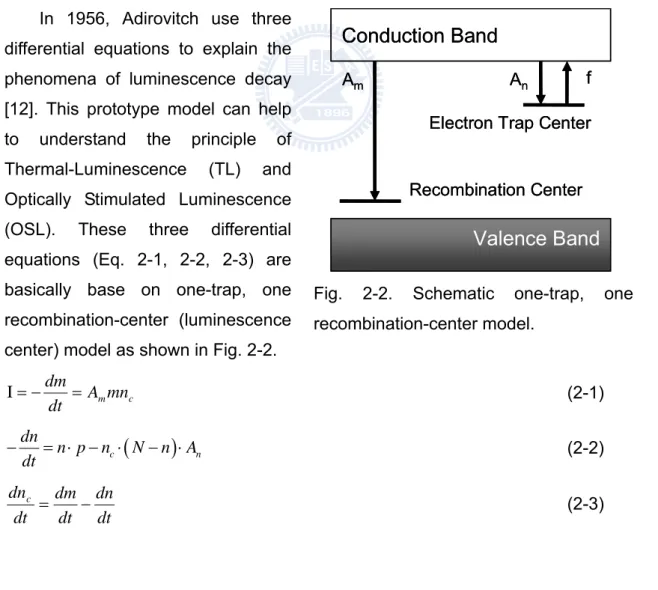
0.5 0.6 0.7 0.8 0.9 1.0 1.1 1.2 0 30 60 90 120 150 S tore days Re lat ive R e spo n se Room temperature

Fig. 1-5. Stable signal of OSL technique for 120 days store (provided by LandauerTM).

(18)

1.3 OSL Application

1.3.1 Personnel Dosimetry

Personnel dosimetry is concerned with the dose evaluation in human body. Deep dose, shallow dose and eye dose are three references parameter in personnel dosimetry. In order to separate different radiation light source effect (like X-rays or gamma-rays) and different human body part effect (different tissue) with those light source, “Absorbed dose” and “Dose equivalent” have been created to quantify the amount of absorption dose for personnel dosimetry.

Absorbed dose refers to the meanenergy, which was imparted by radiation per unit mass of material. The unit of absorbed dose is the “Gray” (Gy). One joule imparted per kilogram of mass is one gray [4].

Dose equivalent refers to the product of absorbed dose of body organ or tissue, which was multiplied by quality factor. The unit of dose equivalent is the “Sievert (Sv)” [4].

Deep dose equivalent refers to the dose equivalent of the external exposure of whole body, including head, trunk, arms above the elbow, and legs above the knee, at depth of 1 cm [4]. By using deep dose as a reference, high energy (such as gamma rays, neutron rays, high-energy beta-particle, X-rays > 15Kev) radiation damage can be estimated.

Shallow dose equivalent refers to the dose equivalent of the external exposure of skin or extremities at tissue depth of 0.007 cm [4]. The interest radiation source here is non-penetrating radiation like low-energy beta particle and X-rays (< 15Kev).

(19)

1.3 OSL Application

Table 1-2. Standard dose calculation Absorbed dose

(Gy)

D = Energy / Mass = Joule / kilogram

(D = absorbed dose in Gy unit) (1-1)

Dose equivalent (Sv)

T T

H

= ×

w D

(w = tissue weighting factor,

T

D = average absorbed dose by tissue)

(1-2)

The gray (symbol: Gy) is the SI unit of absorbed radiation dose due to ionizing radiation (for example, X-rays). The gray measures the deposited energy of radiation. The biological effects vary by the type and energy of the radiation and the organism and tissues involved. The sievert attempts to account for these variations. A whole-body exposure to 5 or more grays of high-energy radiation at one time usually leads to the death within 14 days. Since grays are such large amounts of radiation, medical use of radiation is typically measured in milligrams (mGy).

Gray (Gy) 1 Gy = 1 J/kg = 1 m2_{* s}-2_(1-3)

Sievert (Sv) 1 Sv = 1 J/kg = 1 m2 * s-2 (1-4)

The Sievert (symbol: Sv) is the SI derived unit of dose equivalent. It attempts to reflect the biological effects of radiation as opposed to the physical aspects Gy unit.

Although the “Sievert” has the same dimensions as the “Gray” (i.e. joules per kilogram) in the Eq.1-4 & Eq.1-5, it measures a different quantity. To avoid any risk of confusion between the absorbed dose and the dose equivalent, the corresponding special units, namely the “Gray” instead of the joule per kilogram for absorbed dose and the “Sievert” instead of the joule per kilogram for the dose equivalent, should be used.

(20)

1.3 OSL Application

1.3.2 Environmental Dosimetry

Environmental dosimetry focuses on “man-made” radiation dose around environment. Man-made radiation includes nuclear waste disposal, emission from nuclear power, reprocessing plants and nuclear weapons industry. When the natural radiation over man-made radiation is bigger than 1/1000, long-time monitoring is required to protect our healthy and food. Dosemeter for environmental dosimetry need high sensitivity for low dose detection and need stable reliability under sunlight, weather and temperature exposure. With several “mGy” for nature dose per year, “μGy” dose rate per day require more sensitive technique. Therefore Optically Stimulated Luminescence is the recommendation tool for this short-term monitoring [2].

1.3.3 Radio therapy detection

Although concerned with monitoring radiation exposure for people in the daily life, radiation usage in medical treatment has become a powerful tool when people got cancer. How to qualitatively estimate the amount of dose being used on or in (in vivo) the patient during medical radiation treatment and diagnosis is an important problem. For example, there is a need for small, tiny radiation dosimeters for real-time [5] or near-real-time dose amount readout, including external radiation treatment (X-rays photography) and internal (such as X-ray tubes implanted in a blood vessel). All such applications require dose monitoring to assist in effective treatment. Although TL are popular dosimetric technique in many hospitals for external dosimetry during these treatments. However, the TL can only provide “once” integral reading of the total surface exposure to the patient after treatment. OSL has the potential for the development of “second or more” reading and near-real-time dosimetry [6, 7] by the speed of photon-electron interaction as shown in Fig. 1-6 [8, 9]. The measured quantity of OSL can be either dose (Sv) or dose rate (Sv/s). Typical doses of interest can be up to 20 Sv [3].

(21)

1.3 OSL Application

Nd:YAG Laser PMT Dichroic mirror Fiber Collimator Al₂O₃:C Dosimeter Nd:YAG Laser PMT Nd:YAG Laser PMT Dichroic mirror Fiber Collimator Al₂O₃:C Dosimeter

Fig. 1-6. Schematic picture for real-time radiation therapy by OSL technique. A optical fiber is inserted into a patient and readout the OSL intensity from Al2O3:C on the top of

the fiber. Here, the Nd:YAG Laser is stimulation light source and PMT is photomultiplier tube.

1.3.4 Retrospective dosimetry

Retrospective dosimetry is the dose estimated by environmental or locally available materials instead of conventional synthetic dosimeters. Two major categories exist, namely dating dosimetry and accident dosimetry. Dating dosimetry for geological or archaeological usage using OSL relies upon the determination of the dose absorbed by natural minerals, such as quartz or feldspar [8]. For example, for a windblown deposit (e.g., a sand dune) all previous radiation exposure history (OSL signal) is erased while the sediment grains are being transported in the air where they are exposed to natural sunlight. The erased sediment on the surface of the sand dune was set in “zero dose”. After that, zero dose samples were buried by other sediment grains in the sand dune and shielded the sample from further exposure to sunlight. Therefore, the OSL signal is regenerated by exposure to the environmental radiation field. When the sediment grains are now excavated, the subsequent OSL signal is proportional to the time of burial. Modern techniques use small, single aliquots---even single grains-- and result in large numbers of independent dose determinations. The quantity of interest is the equivalent dose in Gy. This is the beta dose (used for calibration in the laboratory) that yields the equivalent OSL signal to the natural environmental dose, which is derived from a mixed

(22)

1.3 OSL Application

radiation field made up of alpha, beta, gamma, and cosmic radiation.

The other application is accident dosimetry [10]. This is the one that is interested in the determination of absorbed dose due to a radiation accident or other event. Examples include the determination of absorbed doses during events such as nuclear weapons explosions, nuclear reactor accidents or other incidences of unintended radiation release. Because synthetic dosimeters were not in place at the time, one has to rely upon the determination of absorbed doses in locally available materials, such as bricks (in particular the quartz grains within the bricks), or porcelain (light fixtures, bathroom fixtures, etc.). The quantity of interest is the equivalent dose in Gy. OSL is used to be a useful tool because most of the suitable local materials display high OSL intensity.

(23)

1.4 Contribution to this thesis

Dose dependence of Al2O3:C has been

wildly reported in the past decades. However there is a question left. How can we distinguish the Al2O3:C in 5~10Gy or 10Gy

above by the same OSL intensity, as shown in the Fig. 1-7. For nuclear accident, how to estimate the absorption dose of patients who was working in the nuclear power plant or any high radiation environment is a serious problem in dosimetry research, because 5~10Gy is the safe dose amount but dose above 10Gy will cause death.

In the following contents, we will test the reliability of LandauerTM_{POSL reader}

system with LuxelTM _Al

2O3:C badge. Then experimentally use optical bleach method to

distinguish two doses with same OSL intensity. Theoretically, we simulate electron property in Al2O3:C in bleach process and use this simulation for further application.

Fig. 1-7. Demonstration of confusion in dose dependence of Al2O3:C with

same OSL signal [11].

(24)

Part 1- Theory model

Chapter 2 Methods

Part 1- Theory model

2.1.1 Band theorem

OSL signal comes from electron-hole pair recombination. Electron-hole pair recombination happened in OSL material such as semiconductor or insulator. According to quantum mechanism or solid physics, electron behavior in OSL material can be illustrated in band diagram. There is one continuous low energy states, which called valence band and the other one is continuous high energy states, which called conduction band. Between valence band and conduction band, there is some “meta-stable” energy states, which allow the electron live in there temporally.

Fig. 2-1. Band diagram. (1) Ionization (excitation cross the band gap); (2) Exciton formation (3a,3b) Defect ionization; (4a,4b) Trap ionization; (5) Internal intra-band transition.

(25)

Part 1- Theory model

In Fig. 2-1; band-to-band electron behavior (transition 1) occurs in high-energy radiation exposure. Exciton formation (transition 2) is the electron-hole pair formation. It can lead to charge localization and generally occur in superconductivity. Defect ionization (transition 3) always appears in non-well-growth pure material. There are some material distortions or defect where can lead electron to live in that energy level. Trap ionization (transition 4) is caused by impurity in material, such as Al2O3doped

carbon become Al2O3:C. Doped element is another energy level choice for electron to

live in. Intra-band transition (transition 5) combines defect and impurity effect. Therefore, there are some possibilities that electron can jump between defect and impurity [1].

2.1.2 One-trap, one-recombination-center model

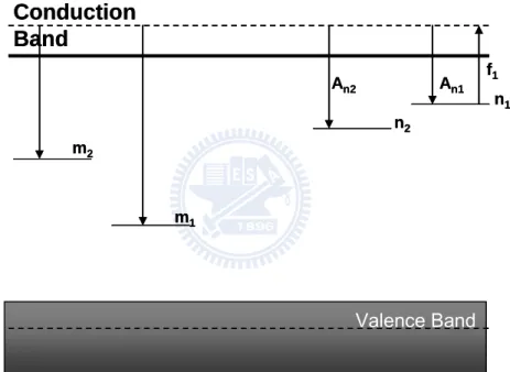
In 1956, Adirovitch use three differential equations to explain the phenomena of luminescence decay

[12]. This prototype model can help us

to understand the principle of Thermal-Luminescence (TL) and Optically Stimulated Luminescence (OSL). These three differential equations (Eq. 2-1, 2-2, 2-3) are basically base on one-trap, one recombination-center (luminescence center) model as shown in Fig. 2-2.

c mmn A dt dm = − = I (2-1)

(

)

c n dn n p n N n A dt − = ⋅ − ⋅ − ⋅ (2-2) dt dn dt dm dt dnc = − _(2-3)

Conduction Band

Valence Band

Recombination Center Electron Trap Center

A_m A_n f

Conduction Band

Valence Band

Recombination Center Electron Trap Center

A_m A_n f

Fig. 2-2. Schematic one-trap, one recombination-center model.

(26)

Part 1- Theory model

The first equation (2-1) demonstrate intensity of luminescence： I：Intensity of luminescence

Am： Probability of electron-hole pair Recombination

m：Concentration of recombination center

nc：Concentration of electron in conduction band

The intensity of luminescence is proportional to recombination center consumption. Therefore, concentration of electron in conduction band and Concentration of recombination center are two factors, which affect the consumption rate of recombination center.

The equation (2-2) demonstrate consumption rate of trapped electron： n：Concentration of trapped electron

N：Maximum concentration of trapped electron An：Re-trap probability

P：Stimulation parameter or pump parameter

The concentration of trapped electron “n” is proportional to radiation dose. Therefore, the variation of trapped electron concentration can estimate the amount of radiation dose; Stimulation parameter “P” is affected by different light source wavelength (cross section) or light source intensity. In this model, the trap has its own maximum concentration “N”. In reality, “N” depends on dosemeter material. By quantum mechanism, the pumped electron will be back to trap state. Therefore, set “An” as re-trap

probability parameter.

The equation (2-3) demonstrates neutrality conditionnc+n=m.

Above equations are first-order dynamics that means variance “n” is first-order. Under first-order dynamics, recombination effect dominates the whole process of luminescence signal.

(27)

Part 1- Theory model

Comparing with the first-order dynamics, the second-order dynamics concerns re-trapping rate as dominator, same concentration condition of recombination center and trap center [13].

2.1.3 Multi-trap, Multi-recombination-center model

In early 2004, non-monotonic dose dependence of TL and OSL had been observed in some of the dosimetric materials [14]. Lawless et al. reported a two-trap & two recombination center model to explain such TL phenomena [15, 16].

In 2006, R. Chen [17] use multi-trap, which has shown in Fig. 2-3, multi-recombination center model to simulate non-monotonic dose dependence of OSL signal in Al2O3:C. This numerical model is used to explain the relationship between OSL

signal intensity “I” and radiation dose “D” is not a linearity line but a parabolic curve as in Fig. 2-4. Valence Band m2 m₁ n2 n1 An1 An2 f₁

Conduction

Band

Valence Band m2 m₁ n2 n1 An1 An2 f₁

Conduction

Band

(28)

Part 1- Theory model

m1：Recombination center (luminescence center) m2：Competitive Recombination center

n1：Dosimetry electron trap center (shallow trap) n2：Competitive electron trap center (deep trap)

According to R. Chen’s claim, one of the traps belongs to dosimetric trap, which could reveal OSL and the other one belongs to competition trap and which has no contribution to emit photons. Similarly, one of the recombination centers is an irradiative center where could produce OSL and another one is a competitive recombination center but with no luminescence emitting. For clear illustration, a schematic diagram is shown in Fig. 2-3.

Fig. 2-4. R. Chen’s simulation compare with experimental data [17] (a) R. Chen’s simulation (b) Experimental data of Al2O3:C [11]

(29)

Part 1- Theory model

2.1.4 Stimulation modulation

Stimulated modulation concerns how to give excitation photon energy. Continuous wave OSL (CW-OSL), linear modulation OSL (LM-OSL), pulsed OSL (POSL) are three different methods as follow：

Fig. 2-5. Schematic representation of the three main OSL stimulation modes, namely: CW-OSL, LM-OSL and POSL [18].

(30)

Part 1- Theory model

2.1.4.1 Continuous wave OSL (CW-OSL)

Continuous-Wave OSL [19] use constant intensity light source to stimulate electron in dosimetric trap and then create luminescence (OSL), as shown in Fig. 2-5. CW-OSL glow curve usually shows exponential decay until it run out of electron concentration in dosimetric trap in Fig. 2-6; Eq. 2-4 is the mathematical express of C.W. light source and always be put into Eq. 2-5 as stimulation term.

φ

(t

)

=

(2-4) ( ) n c d n n A n N n d t = −ϕ σ + − (2-5)

where σ ：Cross section, effect parameter of stimulation light source with wavelength variance

(31)

Part 1- Theory model

2.1.4.2 Linear modulation OSL (LM-OSL)

In 1996, Bulur et. al. introduce an alternative technique of OSL. The intensity of stimulation light source is not constant but ramped linearly [20, 21]. The glow curve measured by using LM-OSL always shows a peak shape. Eq. 2-6 is the mathematical express and always put into trap’s differential equation (Eq. 2-7).

t

γ

φ

(

)

=

(2-6) ( ) n c dn t n A n N n dt = −γ σ + − (2-7)

γ ：Slope of stimulation light source intensity

2.1.4.3 Pulsed OSL (POSL)

There is an experimental drawback of using CW-OSL and LM-OSL. The intensity of continuous stimulation light source is always bigger than that of luminescence signal. This reason increases the difficulty to separate incident photon signal and luminescence photon signal. But using POSL could avoid this noisy effect, because POSL could estimate luminescence signal between time-gap of first pulse and second pulse. It is just a timing-control problem for Photomultiplier Tube (PMT). Another benefit of POSL is the less power consumption comparing with CW-OSL and LM-OSL. Therefore, POSL could avoid noisy signal which caused by thermal-effect. According to above advantage reason, POSL has wild usage in OSL technique.

In mathematical formula, POSL is similar to CW-OSL but has time-gap. The time interval between two pulses should be longer than intrinsic lifetime of the luminescence center as shown in Fig. 2-7.

(32)

Part 1- Theory model

Fig. 2-7. Illustrate timing control of POSL system. (a) The timing relationship between laser pulse, PMT Gate and accumulation of POSL signal (b) Detail in timing control of laser pulse and PMT Gate [1].

(33)

Part 2- Experimental Setup

2.2.1 Characteristic

of

Al

2

O

3

:C

Aluminum oxide Al2O3 is a strong material. It

possesses strong ionic inter-atomic bonding. It can exist in several crystalline phases, which all revert to the most stable hexagonal alpha phase (alpha- Al2O3)

at elevated temperatures [1].

According to absorption spectrum of Al2O3in Fig.

2-9(a), the band gap between conduction band and valance band is nearly 6.0ev [22]. This wind band gap is close to UVA photon energy and OSL device. It also needs to create lower energy state for radiation dose

record. In order to create such “meta-stable” low energy state in 1.0~3.0ev, alpha- Al2O3

will be doped external element carbon and become alpha- Al2O3:C. Fig. 2-9(b)

demonstrates POSL property of Al2O3:C. During the laser pulses case, there are two

peaks exist. One is UVA emission (~340nm). The other one is blue light emission (420nm) [23]. In-between laser pulses, only blue light emission (420nm) appear. In the next section, during laser pulses case is not considered. Because following OSL reader is based on in-between laser pulses.

Fig. 2-9 Optical property of Al2O3:C. (a) Absorption spectrum of Al2O3:C [22] (b)

Emission OSL property of Al2O3:C [23].

<0001> C axis O2 -Al3+ <0001> C axis O2 -Al3+ Fig. 2-8. Schematic of Al2O3 structure

(34)

Part 2- Experimental Setup

2.2.2 LuxelTM OSL Badge of alpha-Al

2

O

3

:C

0.4 mm Cu 0.7 mm Al 0.7 mm Plastic 4 3 2 1 0.4 mm Cu 0.7 mm Al 0.7 mm Plastic 4 3 2 1

Fig. 2-10. Luxel OSL dosemeter (badge).

In the Fig. 2-10, there are four chips in each OSL badge. Outside the four chips, there are three different shielding covers: copper (Cu), alumina (Al) and plastic are used to simulate radiation effects to different parts of human body (Table 2-1). “2D slide code” and “Case bar code” is the record number for experimental note. Standard dose badges from background to 100Gy come from Nuclear Science Center, National Tsing-Hua University, Hsin-chu (Table 2-2).

Table 2-1. The function of four chip in OSL badge

Shielding Material Function

Chip 1 _None Discrimination (standard dose)

Chip 2 0.7mm Plastic Deep dose (10 mm deep below the skin surface) Chip 3 0.7mm Alumina Shallow dose (0.07 mm deep below the skin surface) Chip 4 0.4mm Copper Eye Dose (3mm depth of the lens of eye)

Table 2-2. Luxel badges with standard dose

Dose (Gy) Amount Case Serial#

background 6 _{XA008077692, XA00834036M, XA00669640C}XA00805731N, XA008379254, XA00000570J

1 3 XA008375385, XA000695848, XA008638270

5 3 XA008352888, XA00836603H, XA008389609

10 3 XA00227099F, XA00691630F, XA00867925Y

50 3 XA00061705I, XA00838950A, XA00031544Q

100 3 XA00867979L, XA00254080V, XA008685817

(35)

Part 2- Experimental Setup

2.2.3 Landauer OSL Reader

Fig. 2-11. Landauer InLight System, Automatic 200 unit Reader

In this thesis, a commercially available machine was modified to read the OSL response of the LuxelTM_{dosemeter element. The Luxel dosemeter element used here in}

the study is provided by Landauer, Inc. Although the Luxel element used in the commercial dosimetry service is a pulsed-laser measurement method (POSL), the study here relied on a light emitting diode (LED) readout method in the Landauer InLight reader system.

A cluster of 36 green super-bright LEDs was installed as the excitation source and a Hamamatsu photon-counting photomultiplier tube (PMT) module was installed with appropriate filters to block the green LED light and pass the 420 nm blue OSL emission. The green LEDs had a peak emission wavelength of 525 nm, and the optical power density at the dosemeter was 3mW/cm2_{. The optical filters for the LED light consisted of}

two 515 nm long pass color glass filters. The emission filters cover the PMT window, which consist of a blue band pass filter and a custom interference filter passing 390–450 nm. A basic fast counter was installed to count the pulses from the PMT. The green LEDs were continuously illuminated during the 1 sec measurement time.

(36)

Part 2- Experimental Setup

Height performance PMT 2D for element

BCR for InLight case

2D BCR controller Element push up-units Height performance PMT

2D for element

BCR for InLight case

2D BCR controller Element push up-units

Fig. 2-12. Inside of the Landauer Automatic 200 unit POSL Reader

The sample holder was machined to accommodate the Luxel dosemeter element for completing the readout apparatus. The green LED readout method using OSL-grade alumina was developed in the mid-1990s and the technique was presented at the 1997 annual Health Physics Society meeting [24].

(37)

Part 2- Experimental Setup

PMT PMT LED LED Front knob Front knob PMT PMT LED LED Front knob Front knob

Changer can store 4 magazines and 200 InLight Badge Changer can store 4 magazines and 200 InLight Badge

Fig. 2-13. Illustrate mechanism for Luxel Badge in reading process.

(38)

Part 2- Experimental Setup

2.2.4 Visible Light System

Fig. 2-15. Ultraviolet exposure system for optical bleach experiment.

For qualitative test, a commercial UV lamp was used (6W power and energy center at 350nm belongs to UV-A range, shown in Fig). In the Fig. 2-15, a box and a black bag are used to block visible-light effect from environment. Inside the box, UV lamp always set at 10 cm away from the OSL badge and it has the same vertical height with OSL badge.

Fig. 2-16. The emission spectrum of UVA light tube.(provided by the website of http://www.100y.com.tw/pdf_file/SANKYO_BLACKLIGHT-BLUE.pdf)

(39)

Part 2- Experimental Setup

2.2.5 Ultraviolet System

Fig. 2-17. Experimental setups for visible light bleach.

For another qualitative bleach test, 5 parallel visible light sources were used (18W*5 =90W PHILIPS MASTER TL-D Super 80 /840 SLV) in the Fig. 2-17. The spectrum of each light source is centered at 420nm (blue), 560nm (Green) and 640nm (Red), combine 3-band fluorescence as shown in the Fig. 2-18. Under 18 cm of the light source, irradiation platform was designed for OSL badge bleach with UV filter to avoid UV effect (less than 40% below 370nm) shown in the Fig. 2-19.

Fig. 2-18. The emission spectrum of visible light source. (provided by the website of http://www.philips.com.tw)

(40)

Part 2- Experimental Setup

(41)

3.1 Standard deviation

Chapter 3 Experimental Result

3.1 Standard deviation

Four standard badges (1mGy, 1Gy, 5Gy, and 10Gy) were used to evaluate the stability and reliability of LuxelTM badge under 0.01mGy error reliability of Landauer POSL reader. Usually, the one year background accumulation dose is approximately approached to 1 mGy and to map the value to 150 Convertible Value (Conv. Val.) in the Landauer POSL reader. According to Fig. 3-3 and Fig. 3-4, badge has nearly 4.6% error dose. It is acceptable due to the value is less than 0.05mGy which is half-month background accumulation dose. About 1Gy (=56000 Conv. Val.) badge, has nearly 5.3% error dose. 5Gy (=316000 Conv. Val.) badge, has nearly 5.8% uncertainty. 10 Gy (=716000 Conv. Val.) badge has nearly 3% fluctuation.

LuxelTM_{badges be exposed to}

standard dose from 1Gy to 10Gy and background dose

Using Landauer OSL reader continuously read out OSL intensity variation for 40 times

Draw the dose dependence of OSL intensity picture and calculate the standard deviation as the error bar of follow chart

LuxelTM_{badges be exposed to}

standard dose from 1Gy to 10Gy and background dose

Using Landauer OSL reader continuously read out OSL intensity variation for 40 times

Draw the dose dependence of OSL intensity picture and calculate the standard deviation as the error bar of follow chart

Fig. 3-1. Flow chart for Landauer OSL reader reliability test.

(42)

3.1 Standard deviation

Fig. 3-2. Average distribution of 1, 5, 10, 50, 100Gy for 40 Times OSL Read out.

Fig. 3-3. Standard deviation of four elements in background and 1Gy Badge.

(43)

3.1 Standard deviation

Standard Deviation of nonlinear dose dependence-50 Gy

The OSL signal (Conv. Val.) start to non-steady severe fluctuated when the dose was increased to extremely high dosage, i.e. above 50Gy. This means standard deviation have become worse. Fig. 3-5 is three 50Gy badges OSL intensity varies with 40 times read out. Apparently, two badges (XA00061705I & XA00838950A), in Fig. 3-5 have two layers to separate element 1 and element 2, 3, and 4. The main reason of this phenomenon could attribute to LuxelTM badges shielding (chapter 2). The 50Gy (=436000 Conv. Val.) badge, has nearly 16% uncertainty so that the factor is significant parameter to distinguish 5~10Gy and above 10Gy to 50Gy. Although, the OSL intensity (Conv. Val.) of 5~10Gy and 10~50Gy is similar to 450000~550000 Conv. Val. comparing Fig. 3-4 and Fig. 3-5, the uncertainty is 5% and 16% respectively. For reliable data analysis, element-1 in XA00838950A is taken into consideration for numerical analysis reference point.

Fig. 3-5. 40 times readout distribution and standard deviation of four elements in three 50Gy Badges.

(44)

3.1 Standard deviation

Fig. 3-6. 40 times readout distribution of 5Gy & 10Gy.

Standard Deviation of nonlinear dose dependence-100 Gy

When the amount of dose increase to 100Gy, the OSL intensity (Conv. Val.) fluctuate more violently. In Fig. 3-7, the uncertainty of 100Gy badge is roughly 12.5%, 24%, 26% for XA00867979L, XA00254080V, XA008685817 respectively. Although the 100Gy OSL intensity seems very vague, the intensity (Conv. Val.) still locate in the same range of 5~10Gy. Therefore, there is a question left behind： How can we distinguish the badge is 5~10Gy or 50~100Gy by using the same Convertible Value?

Fig. 3-7. 40 times readout distribution and standard deviation of four elements in three 100Gy Badges.

(45)

3.2 Visible light effect

A visible light bleach system was designed (In chapter 2) to separate 5~10Gy and 10~50Gy badge. Each standard-dose badge was exposed under visible light tubes with UV filter for 3~10 min respectively. The result in Fig. 3-8 shows different decay speed during 10 min exposure. For example, XA008389609 (5Gy) & XA00061705I (50Gy) are at the beginning. For 10 min visible light bleach, the slope of 5Gy and 10Gy OSL variation is smaller than that of 50Gy and 100Gy. To further verify the validation of the study, exceed 10 min bleaching is needed for avoiding signal jumping, which is shown in Fig. 3-8. According to this bleach result, a critical slope value could be set to determine the dose in both high and low range. For easy slope recognition, exposure in 10 to 20 minutes is suggested.

Fig. 3-8. Visible Light Bleach effect for 5~100Gy Badge

The inset picture of Fig. 3-8 shows that the decay speed (slope) of 100Gy badges is slower than 5~10Gy. No matter how wide the range of OSL initial intensity it is, visible light bleach can still do the function to determine the badge 5~10Gy or above 10Gy.

0 100000 200000 300000 400000 500000 600000 700000 800000 900000 0 10 20 30 40 Time (min) Ele me n t-1 C onv. Va l. XA00254080V (100Gy) XA00867979L (100Gy) XA008685817 (100Gy)

(46)

3.2 Visible light effect

0 20 40 60 80 100 -10 0 10 20 30 40 50 60 70 80 90

Element-2 Conv. Val. (10

4 count) Dose (Gy) Time = 0 min Time = 10 min Time = 20 min 0 20 40 60 80 100 -10 0 10 20 30 40 50 60 70 80 90

4 count) Dose (Gy) Time = 0 min Time = 10 min Time = 20 min 0 20 40 60 80 100 -10 0 10 20 30 40 50 60 70 80 90 Element-3 C o n v . Val. (10 4 count) Dose (Gy) Time = 0 min Time = 10 min Time = 20 min 0 20 40 60 80 100 -10 0 10 20 30 40 50 60 70 80 90

4 count)

Dose (Gy)

Time = 0 min Time = 10 min Time = 20 min

Fig. 3-9. The Visible light Bleach effect for Element 1,2,3 and 4.

Figure 3-9 demonstrates that bleach effect in four elements for each badge is similar. There is no need to see four elements bleach effect in the following text. The first element will be use as experimental reference data for simulation analysis.

(47)

3.3 UV light effect

A UV light bleach result is displayed in Figure 3-10. Two background dose (nearly under 200 Conv. Val. = under 1mGy) badges were exposed to UV. The “step” in horizontal axis stands for 3 min UV exposure. Form “step1” to “step8”, a pump effect was discovered. “step8” to “step9” is that badges were laid on the table without UV exposure. Form “step9” to “step11”, another pump effect was discovered too. It means UV light for LuxelTM Al2O3:C badge not only has “bleach effect” (Fig. 3-11), but also has

“pump effect” (Fig. 3-10).

0 1 2 3 4 5 6 7 8 9 10 11 12 0 50 100 150 200 250 300 350 400 450 500 Element-1 C o nv. Val. Step XA00000570J (Background) XA00805731N (Background) 0 1 2 3 4 5 6 7 8 9 10 11 12 0 50 100 150 200 250 300 350 400 450 500 Element-1 C o nv. Val. Step XA00000570J (Background) XA00805731N (Background)

Fig. 3-10. UV light pumping effect for background dose badge.Note that each “step” stands for 3 min UV exposure and “step8” to “step9” is 12 hours.

0 2 4 6 8 10 0 100000 200000 300000 400000 500000 600000 Element-1 Conv . Val. Dose (Gy) Before 1 Hour UV Bleach After 1 Hour UV Bleach

(48)

4.1 Set differential equation

Chapter 4 Simulation and Discussion

4.1 Set differential equation

Chapter 2 has already introduced how to use band diagram to describe electron behavior in the Al2O3:C and how to write down the

ordinary differential equation (ODE) according to band diagram. As ODE is a dynamic system, choosing a proper numerical method must be considered. After that, tune the parameter in each ODE because each parameter has its own physical probability meaning. Finally, compare the simulation data with experimental data. Checking if they match or not, if not we should modify band diagram or tune a new set of parameters, as shown in Fig. 4-1.

Put ODE into Matlab 2007 software and use “ode23” to solve this dynamic simulation Writing down proper

Ordinary Differential Equation (ODE)

Tune the parameter in the ODE and compare with experimental result

Put ODE into Matlab 2007 software and use “ode23” to solve this dynamic simulation Writing down proper

Ordinary Differential Equation (ODE)

Tune the parameter in the ODE and compare with experimental result

Fig. 4-1. The flow chart of simulation process.

(49)

4.1 Set differential equation

There are four steps (Fig. 4-2) or four strategies to describe electron behavior in the Al2O3:C. First, simulate Al2O3:C under high

energy radiation explosion such as X-rays or beta-rays. Follow that, the system has to obey thermal equilibrium process. Electrons in this step should be distributed to another state by thermal energy. Theoretically, ODE dynamic system should be added with some thermal excitation term. Third, writing down a set of bleach ODE by adding bleach factors to simulate electron for pumping away electrons from the original states. Finally, same as bleaching step, POSL also need to pump away electrons in dosimetric trap. Thus, change bleach factors to POSL bleach factors. Then read out the concentration variance to calculation OSL intensity (so called “glow curve”).

Valence Band m₂ m₁ n2 n1 A_n1 A_m1 A_m2 _A n2 f1 B2 B1 X Conduction Band Valence Band m₂ m₁ n2 n1 A_n1 A_m1 A_m2 _A n2 f1 B2 B1 X Conduction Band

Fig. 4-3. Schematic R. Chen’s multi-trap, multi-recombination-center energy model.

The used model is shown in Fig. 4-3, N1 which is an “active” dosimetric trap, meaning that the stimulating light is capable of releasing electrons from it, and N2, a competitor, which the electrons can be trapped, but the stimulating light cannot release

1. Material be bombarded with high energy radiation 2. Thermal Equilibrium 3. Optical Bleach 4. Optical stimulated Luminescence (OSL) 1. Material be bombarded

with high energy radiation

2. Thermal Equilibrium

3. Optical Bleach

4. Optical stimulated Luminescence (OSL)

Fig. 4-2. The steps of ordinary differential equation in Matlab 2007 software.

(50)

4.1 Set differential equation

electrons from it. Two recombination centers are assumed to exist, M1, radioactive center, and M2 a non-radioactive competitor. The set of six coupled differential equations are governing each process. The repeated simulation of R. Chen’s is in the figure 4-4.

Bombard with high energy radiation

c n

N

n

A

dt

dn

)

(

₁ ₁ 1 1

=

−

_(3-1) c n

N

n

A

dt

dn

)

(

₂ ₂ 2 2

=

−

(3-2) 1 1 1 1

(

1 1

)

m c v

d m

A m n

B

M

m

n

d t

= −

+

−

(3-3) 2 2 2 2

(

2 2

)

m c v

dm

A

m n

B

M

m

n

dt

= −

+

−

(3-4) 2

(

2 2

)

1

(

1 1

)

v v v

dn

X

B M

m

n

B M

m n

dt

=

−

(3-5) 1 2 1 2 c v d n d m d m d n d n d n d t = d t + d t + d t − d t − d t (3-6)

Physical description Unit

M1 The concentration of radioactive hole centers (cm−3) M2 The concentration of non-radioactive hole centers (cm−3)

m1 Instantaneous occupancy (cm−3)

m2 Instantaneous occupancy (cm−3)

N1 The concentration of the electron active trap state (dosimetric

trap, shallow trap)

(cm−3)

N2 The concentration of the trapping state (cm−3)

n1 Instantaneous occupancy (cm−3)

n2 Instantaneous occupancy (cm−3)

nc The concentrations of the electrons in the conduction bands (cm−3) nv The concentrations of holes in the valence bands (cm−3)

(51)

4.1 Set differential equation

X The rate of production of electron-hole pairs, which is

proportional to the excitation dose rate

(cm−3)(s−1)

B1,

B2

The trapping probability coefficients of free holes in Recombination centers 1 and 2

(cm−3_)(s−1₎

Am1,

Am2

Recombination probability coefficients for free electrons with holes in centers 1 and 2,

(cm−3)(s−1)

An1 The re-trapping probability coefficient of free electrons into the

active trapping state N1 (dosimetric trap)

(cm−3)(s−1)

An2 The trapping probability coefficient of the free electrons into

the competing trapping state N2

(cm−3_)(s−1₎

(X*T) If we denote the time of excitation by (T) and the rate of production of electron-hole pairs per cm3 by (X), then represents the total concentration of electrons and holes produced, which is proportional to the total dose imparted.

Gy, Sv

f A magnitude proportional to the stimulating light source

intensity. (s

−1₎

Thermal Equilibrium condition

c n

N

n

A

dt

dn

)

(

₁ ₁ 1 1

=

−

_(3-7) c n

N

n

A

dt

dn

)

(

₂ ₂ 2 2

=

−

(3-8) 1 1 1 1

(

1 1

)

m c v

d m

A m n

B

M

m

n

d t

= −

+

−

(3-9) 2 2 2 2

(

2 2

)

m c v

dm

A

m n

B

M

m

n

dt

= −

+

−

(3-10) 2

(

2 2

)

1

(

1 1

)

v v v

dn

B M

m n

B M

m n

dt

= −

−

(3-11) 1 2 1 2 c v d n d m d m d n d n d n d t = d t + d t + d t − d t − d t (3-12)

(52)

4.1 Set differential equation

Optically Stimulated processes

c n

N

n

A

fn

dt

dn

)

(

1 1 1 1 1

=

−

+

−

_(3-13) c n

N

n

A

dt

dn

)

(

₂ ₂ 2 2

=

−

(3-14) 1 1 1 m c

dm

A m n

dt

= −

(3-15) 2 2 2 m c

dm

A m n

dt

= −

(3-16)

0 =

dt

dn

_v (3-17) 1 2 1 2 c v

d n

d m

d n

d t

=

d t

+

d t

+

d t

−

d t

−

d t

(3-18)

Luminescence

c m

m

n

A

dt

dm

t

I

₍

₎

=

−

1

=

₁ ₁

,

I(t)：OSL Intensity or Glow curve (3-19)

∫

I(t)dt = m₁₀ − m₁_f (3-20) 0 0.5 1 1.5 2 2.5 0 2 4 6 8 10 log10(Dose) R adi at iv e C en ter O cc upanc y / I nt egr al O S L m10 m1f m10-m1f

Fig. 4-4. Repeat R. Chen’s simulation result. The right side of the figure is the simulation of integral OSL versus dosimetry (log scale) and is fully matched with the result of R Chen’s proposed (left side) [10].

(53)

4.2 Modification

4.2.1 Bombard with high energy radiation

The main OSL emission band at ~420nm (Akselrod et al., 1990 [26]; Markey et.,1995 [27]) is attributed to radioactive relaxation of excited F-centers, which are created after electron recombination with F+-centers (Springis et al., 1995 [28]). When F-center accepts 206nm UV light, it will convert back to F+ center (F-center + 206 nm Æ F+-center + e-). F+ center is the luminescence center in Al2O3:C [29]. It is one of

dominate factors for OSL intensity. Thus back to R. Chen’s model, we modified Eq.3-3 & Eq.3-4 to Eq.3-25 & Eq.3-26 respectively and added C m n and 1 2 c C m n into the 2 2 c

equations. These two terms represent the probability that F-center (M2) would accept enough high energy and become F+-center (F-center + high energy (beta-rays) Æ F+-center + e-). The phenomena depends on m2 concentration (F-center) and electron concentration nc. Conversion rate C1 was set equal to C2 with opposite sign. This setting represents the 100% F-center conversion will change to F+-center. Figure 4-5 is C1 & C2 parameter simulation. This figure shows the F-center conversion must occur in the Al2O3:C. Comparing with Figure 4-5(b), experimental result, we chose C1 = C2 = 50

for the following simulation.

1 1 1 1

(

1 1

)

1 2 m c v c

d m

A m n

B

M

m

n

C m n

d t

= −

+

−

+

(3-25) 2 2 2 2

(

2 2

)

2 2 m c v c

dm

A

m n

B

M

m

n

C m n

dt

= −

+

−

(3-26)

(54)

4.2 Modification

0 20 40 60 80 100 0 5000 10000 15000 20000 25000 30000 35000 40000 R e latice O S L Intes ity / O S L Count Dose (Gy) C1 = C2 = 100 C1 = C2 = 50 C1 = C2 = 25 C1 = C2 = 0

Fig. 4-5. (a)F-center conversion simulation result and (b) experimental data.

4.2.2 Optical

Bleach

The mathematical term(−V nf) 1 was set into n1 state, same as in the set of

equations for OSL process. This is base on the assumption that visible light only cleans electrons in the dosimetric trap and there is no enough energy to bleach electrons in deep trap. The simulation result is shown in Fig 4-6. Point “A “to “H” is the experimental data and they are roughly match our simulation result in Fig. 4-6, Fig. 4-7 and Fig. 4-8.

1 1 1 1 1

(

_f

)

_n

(

)

_c

dn

V

n

A

N

n n

dt

= −

+

−

(3-27) A B C D E F G H A B C D E F G H A B C D E F G H A B C D E F G H

(55)

4.2 Modification

0 100000 200000 300000 400000 500000 600000 700000 800000 0 2 4 6 8 10 Dose (Gy) El em ent -2 C onv. V al . Time = 0 Time ~ 10 min Time ~ 20 min

Fig. 4-8. Detail bleach effect of optical bleach effect in 1~ 10Gy with simulation result. Fig. 4-7. Simulation matches the OSL decay speed with different dose.

0 5 10 15 20 0 0.5 1 1.5 2 2.5 3x 10 4 Time (min) O S L R el at iv e I nt ens ity / O S L C ount 5Gy 10Gy 50Gy 100Gy

(56)

4.2 Modification

4.2.3 Maximum

Bleach

Fig. 4-9. Bleach effect with UV filter in the visible light system.

In the personnel dosimetry and environmental dosimetry, maximum bleach for badge is very important. Both of dosimetry estimate dose range in mGy range. Figure 4-9 and figure 4-10 are under visible light system with UV filter and without UV filter respectively. With UV-filter and 10 min exposure case, the dose of badge will decrease to 0.1 mGy (=10 Conv. Val.) as shown in Fig. 4-10. On the other hand, in Fig. 4-11 without UV-filter, the dose of badge will left 0.2 mGy (=20 Conv. Val.). This phenomenon describes UV light in the visible light tube will increase dose in the badge. In physical explanation, UV light source can not only bleach electrons trap center but also add extra electron into trap center. Therefore, ODE dynamic system should be modified as following: 1 1 1 1 1 1

(

f

)

(

v

)

n

(

)

c

dn

V

n

U

n A

N

n n

dt

= −

+ −

−

(3-28) 2 1 2 2 2

(

_v

)

_n

(

)

_c

dn

U n

A

N

n n

dt

= −

+

−

(3-29) 1 1 1

(

)(

1 1

)

m c v

dm

A m n

U

M

m

dt

= −

+

−

(3-23)

(57)

4.2 Modification

For UV light could pump electrons from dosimetric trap and deep trap, (−U nv) 1was

written into N1 state and N2 state in the ODE, where Uv is the coefficient of UV impact factor. On the other hand, UV light also could add electron into dosimetric trap and deep trap. Therefore, (Uv)(M1−m1) was put into M1 state. In order to determine the

simulation parameter Uv and Vf, , we calculate minimum photon unit by bleach light

source spectrum intensity (Fig. 2-16&2-18) and then estimate photon number of wavelengths. We assume 400nm is a critical wavelength between bleach and pump effect. Moreover, we set 50 to 50 percentages for UV pump and bleach effect respectively. Finally, set the simulation parameter of bleach photon number of visible light as 0.5 and others proportional to this value. The simulation result is shown in Fig. 4-12.

Table 4-1. Calculation of lowest common multiple for bleaching photon 420nm = 2.95ev, 560nm=2.21ev, 640nm=1.93ev, 1ev = 1.6*1019J 90W*60sec=5400J

Visible

Lamp 5400J/(80*3.1+200*2.95+400*2.21+350*1.93)/1019_=2.25714*1019

(Minimum photon unit for visible light) 350nm=3.54ev, 1ev = 1.6*1019_J

4w*60sec=240J UV Lamp

240J/3.54/1019=6.7796*1020

(Minimum photon unit for UV lamp)

154 16 167 24 22 24 16 18 19 13 17 17 ₁₉ 20 13 19 167 17 0 20 40 60 80 100 120 140 160 180 0 1 2 3 4 5 6 Step Number E lem ent-1 C onv. Val . XA00000570J XA00834036M XA00669640C

(58)

4.2 Modification

Table 4-2. Simulation parameter dependence Photon Number UV (<400nm) Visible(>400nm) UV pump (50%) UV bleach (50%) 40*2.25*1019=9.02*1020 40*2.25*1019=9.02*1020 (200+400+350)* 2.25*1019 =2.14*1022

Simulation Simulation Simulation

Visible Lamp 0.021 0.021 0.5 0.5*6.77*1020=3.38*1020 _0.5*6.77*1020_=3.38*1020 Simulation Simulation UV Lamp 0.007 0.007 0 10 20 30 40 50 0 10000 20000 30000 40000 50000 R e lati ve OSL Inten sity / O S L Co un t Time (min) n10 = 15000 n10 = 30000 n10 = 60000 0 10 20 30 40 50 0.0 0.1 0.2 0.3 0.4 0.5 0.6 0.7 0.8 0.9 1.0 1.1 1.2 1.3 N o rm al ized Rel ati v e O S L I n ten sit y / O S L C o u n t Time (min) Uv = 0.021, Vf = 0.5+0.021,Without UV filter Uv = 0.004, Vf = 0.504,With UV filter

Fig. 4-11. Bleach effect will achieve to a saturation point.

Fig. 4-12. Different light source has different saturation point.

The simulation results are shown in Figure 4-11 and Fig. 4-12. It successfully explains UV bleach effect with pumping function and the OSL intensity saturate at the same place. In Fig. 4-11, different n1 initial concentration represents different

experimental condition in Fig. 4-9. The other simulation result in Fig. 4-12 demonstrates different bleach light source has different saturation effect. This simulation explain even though Visible light tube is for bleach usage, but it also has pumping factors to achieve low saturation. Therefore, UV filter usage in visible light system is necessary for deep bleach in OSL badge.

基於光刺激發光技術用於Al2O3:C材料之劑量消光研究

國 立 交 通 大 學

電 子 物 理 研 究 所

碩士論文

基於光刺激發光技術用於 Al

O

:C 材料之劑量消光研究

Optical Bleach For Dosimetry in Al

O

:C Base On

Optically Stimulated Luminescence Technique

研 究 生：李 勁 吾

指導教授：謝 奇 文 博士

基於光刺激發光技術用於 Al

O

:C 材料之劑量消光研究

Optical Bleach For Dosimetry in Al

O

:C Base On Optically Stimulated

Luminescence Technique

研 究 生：李 勁 吾 Student：Jing-Wu Li

指導教授：謝 奇 文 教授 Advisor：Prof. Chi-Wen Hsieh

國 立 交 通 大 學

電 子 物 理 所

碩 士 論 文

基於光刺激發光技術用於 Al

O

:C 材料之劑量消光研究

學生：李 勁 吾 指導教授：謝 奇 文 教授

國立交通大學電子物理所碩士班

摘 要

為了解決 Al

O

:C 材料在同一光激發螢光強度下對應兩個高低不同的

輻射劑量值問題，本文嘗試使用部分光清除方法，得到在相同照射時間下

光激發螢光強度有不同的下降速率，於是高低兩個值分開。

實驗上利用可見光和紫外光作為光清除燈源，發現紫外光有清除能力

但也有累積劑量的效果。

理論上利用了能帶理論模擬電子在 Al

O

:C 材料中的光清除行為，和最

大光清除效果。模擬結果和實驗值比對，進而以此數學模型預測激發光源

調變後材料 Al

O

:C 的發光行為變化。

Optical Bleach For Dosimetry in Al

O

:C Base On Optically

Stimulated Luminescence Technique

Student：Jing-Wu Li Advisor：Prof. Chi-Wen Hsieh

Department of Electrophysics

National Chiao Tung University

Abstract

誌 謝

TABLE OF CONTENTS

List of Figures

List of Tables

1.1 Background

Chapter 1 Introduction

1.1 Background

1.2 OSL vs. TL

1.2 OSL vs. TL

1.2 OSL vs. TL

1.2 OSL vs. TL

1.2 OSL vs. TL

1.2 OSL vs. TL

1.3 OSL Application

1.3 OSL Application

1.3.1 Personnel Dosimetry

1.3 OSL Application

D = Energy / Mass = Joule / kilogram

H

= ×

w D

1.3 OSL Application

1.3.2 Environmental Dosimetry

1.3.3 Radio therapy detection

1.3 OSL Application

1.3.4 Retrospective dosimetry

1.3 OSL Application

國立交通大學

電子物理研究所

研究生：李勁吾

指導教授：謝奇文博士

研究生：李勁吾 Student：Jing-Wu Li

指導教授：謝奇文教授 Advisor：Prof. Chi-Wen Hsieh

國立交通大學

電子物理所

碩士論文

學生：李勁吾指導教授：謝奇文教授

摘要

誌謝