基於內視鏡影像序列之手術器械辨識與追蹤

國立交通大學

電控工程研究所

碩士論文

基於內視鏡影像序列之手術器械辨識與追蹤

Surgical Instrument Recognition and Tracking

Using Endoscopic Image Sequences

研 究 生：陳俊儒

指導教授：宋開泰 博士

基於內視鏡影像序列之手術器械辨識與追蹤

Surgical Instrument Recognition and Tracking

Using Endoscopic Image Sequences

研 究 生：陳俊儒

Student: Chun-Ju Chen

指導教授：宋開泰 博士

Advisor: Dr. Kai-Tai Song

國 立 交 通 大 學

電 控 工 程 研 究 所

碩 士 論 文

A Thesis

Submitted to Institute of Electrical Control Engineering College of Electrical and Computer Engineering

National Chiao Tung University in Partial Fulfillment of the Requirements

for the Degree of Master in

Electrical Control Engineering July 2013

Hsinchu, Taiwan, Republic of China

i

基於內視鏡影像序列之手術器械辨識與追蹤

學生:陳俊儒 指導教授:宋開泰 博士 國立交通大學電控工程研究所

摘要

本論文主旨在研究內視鏡扶持機器人之影像追蹤系統。內視鏡裝置於扶持機 器人上，本系統會透過內視鏡的影像即時偵測手術器械，並根據器械在影像上的 位置自主調整內視鏡扶持機器人運動，帶動內視鏡的移動以提供適當的影像視野。 在影像辨識設計部份，本論文提出基於Spiking Neural Network(SNN)演算法，利 用手術器械之紋理和幾何等自然特徵來辨識內視鏡影像中之手術器械。透過資料 訓練後，類神經網路辨識器不容易受光線變化所影響；器械的大小變化或形變等 辨識問題也能被克服。本論文結合Region of interest及Kalman filter估測影像畫面 中器械之位置以提升辨識的效率。在手術器械追蹤控制方面，考慮到內視鏡對器 械的追蹤太過敏感會導致手術中螢幕影像畫面過度晃動而干擾醫師，我們提出 「緩衝區」的設計，以進行手術器械之追蹤控制。如此一來，內視鏡機器人在追 蹤器械的同時，也能提供穩定的影像畫面。所發展之方法先以內視鏡影像驗證器 械之辨識率可達91%以上; 進而在華陀機器人上進行影像追蹤實驗，成功驗證本 論文所發展方法之有效性。

ii

Surgical Instrument Recognition and Tracking

Using Endoscopic Image Sequences

Student: Chun-Ju Chen Advisor: Dr. Kai-Tai Song

Institute of Electrical Control Engineering National Chiao Tung University

Abstract

The objective of this study is to design an image tracking algorithm for the endoscopic system in Minimally Invasive Surgery (MIS). The endoscopic robot autonomously adjusts its pose according to the position of the instruments in image plane, and moves the endoscope to provide a suitable field of view. A method is proposed to identify the tip of instruments without using extra artificial markers. We suggest to use texture and geometric features of laparoscopic instruments and to adopt the spiking neural network approach for object detection. Affection of light change can be reduced. The size change problem and deformation of the instrument can be handled by the neural network. To enhance tracking performance, we further employ region of interest(ROI) and Kalman filter to the neuro-based tracker. For the tracking control of surgical instrument, we propose to set a buffer zone in the center of the image frame to avoid redundant movement of the camera. In this way, the endoscopic system provides a stable view while the robot is tracking surgical instruments. By using endoscopic images, a recognition rate above 91% has been achieved for surgical instruments. Practical experiments on Huatuo robot further validate the effectiveness of the developed image tracking methods.

iii

誌謝

感謝我的指導老師宋開泰教授在這兩年的指導，在論文方面不遺餘力地給予 建議與指導研究方向，在寫作方面也不厭其煩地給予意見與修正，讓本論文得以 順利完成。在待人處事方面，老師也會教導我應有的態度與自我要求，使我受益 良多。 接著，必須感謝口試委員歐陽盟教授、劉楷哲主任及顏炳郎教授對本論文的 建議與指引，強化本論文的嚴整性與可讀性。此外，也要感謝秀傳亞洲遠距微創 手術中心及彰濱秀傳紀念醫院對本論文在實驗上的支持與協助。特別感謝劉楷哲 主任、賀友林高專、王民良博士、夏夢麟博士、陳立珣放射師、邱雅婷助理，以 及研究員汪彥佑、吳景仁等影像部門的所有人在實驗過程所給予的協助，還有很 多生活方面的照顧，讓我在秀傳實驗時都能夠一切順利。 感謝已畢業的嘉豪學長曾對於本論文的建議與討論，也感謝學長格豪、信毅、 允智、仕晟、建宏、上畯、家昌、章宏、學姊巧敏在過程中的協助，以及感謝同 學昭宇和京叡及依穎在學習過程中互相勉勵與成長，同時感謝學長育萱、學弟瑋 哲、明翰、佑霖、奕夫、政輝、炳勳、尚陽、泓文、威翔在生活與課業帶來的樂 趣。 另外，特別感謝我的父母與姊姊，不論是在生活上的支援或是精神上的關心 與鼓勵，都是我繼續前進的動力。由於他們的栽培，讓我得以有豐富的學習資源， 在此我願以此論文獻給我最摯愛的父母與姊姊。

iv

Contents

摘要... i Abstract ... ii 誌謝... iii Contents ... iv List of Figures ... vi

List of Tables ... viii

Chapter 1 Introduction ... 1

1.1 Motivation ... 1

1.2 Related Work... 2

1.3 Spiking Neural Network... 6

1.4 Problem Statement ... 8

1.5 System Overview ... 10

Chapter 2 Laparoscopic Instrument Detection ... 12

2.1 Proposed Instrument Detection Architecture ... 12

2.2Model of Spiking Neural Network ... 12

2.2.1 The First Layer of the Network ... 15

2.2.2The Second Layer of the Network ... 17

2.2.3Network Learning ... 18

2.2.4 Object Recognition ... 20

2.3 Object Recognition under Complex Environment ... 23

2.4 Kalman Filter Design ... 26

Chapter 3 Image Tracking System ... 32

3.1 Buffer Zone Design ... 32

v

3.3 Motion Control of Robotic Arm... 36

Chapter 4 Experimental Results ... 39

4.1 Experiment by Using In-vivo Endoscopic Video ... 39

4.1.1 Data Training of the Instruments ... 39

4.1.2 Instruments Recognition by Using Video ... 41

4.2 Experiment of Visual Servo by Endoscopic Robot ... 42

4.2.1 Experimental Setup... 42

4.2.2 Image tracking on Robotic Platform ... 45

4.3 Discussion in the Experiments ... 49

Chapter 5 Conclusion and Future Work ... 52

5.1 Conclusion ... 52

5.2 Future Work ... 53

vi

List of Figures

Fig. 1.1 Marker spots used for recognition and 3D pose estimation.[9] ... 3

Fig. 1.2 Instrument detection by using particle filter.[11] ... 3

Fig. 1.3 Recognize the type of the instrument[12] ... 4

Fig. 1.4 3D pose estimation by fitting contour with 3D model in data base.[13] ... 4

Fig. 1.5 Tracking in the occluded condition.[14] ... 5

Fig. 1.6 Instrument detection by metallic color and k-means.[15] ... 5

Fig. 1.7 Find the tip of the instrument by the straight edge.[16] ... 5

Fig. 1.8 Combine gradient-base tracker and classifier-based detector for tracking.[18] ... 6

Fig. 1.9 Schematic diagram of spike train.[21] ... 7

Fig. 1.10 Visual signal transduction. [22] ... 7

Fig. 1.11 Robotized surgical instruments of Da Vinci system[27]. ... 9

Fig. 1.12 System architecture. ... 10

Fig. 2.1 Image tracking algorithm. ... 13

Fig. 2.2 Architecture of spiking neural network. ... 14

Fig. 2.3 LoG kernels. ... 15

Fig. 2.4 Schematic diagram of image convolution. ... 16

Fig. 2.5 LoG kernel operation. ... 16

Fig. 2.6 Gabor kernels. ... 17

Fig. 2.7 Gabor kernel operation ... 18

Fig. 2.8 Training of the spiking neural network. ... 19

Fig. 2.9 The schematic diagram of target kernel generation. ... 20

Fig. 2.10 The process of the recognition value in output layer. ... 21

Fig. 2.11 Rank-order-coding scheme. ... 22

vii

Fig. 2.13 Neural contribution in equation (2.7). ... 24

Fig. 2.14 Image tracking under complex background. ... 26

Fig. 2.15 Instrument tracking using Kalman filter. ... 30

Fig. 3.1 Schematic diagram of buffer zone. ... 32

Fig. 3.2 The ratio of buffer zone. ... 33

Fig. 3.3 The flow chart of motion control. ... 34

Fig. 3.4 Two operation modes of laparoscopic instruments tracking. ... 34

Fig. 3.5 Specific condition that would be misjudged. (a)Top view, (b)Side view. ... 36

Fig. 3.6 Control architecture of surgical instrument tracking. ... 37

Fig. 4.1 Snapshot from in-vivo endoscopic video. ... 39

Fig. 4.2 Training samples of the right instrument. ... 40

Fig. 4.3 Training process of the right instrument. ... 40

Fig. 4.4 Training samples of the left instrument. ... 40

Fig. 4.5 Lighting variation condition. ... 41

Fig. 4.6 Size change condition. ... 41

Fig. 4.7 Hardware architecture. ... 43

Fig. 4.8 The tip of endoscope. ... 43

Fig. 4.9 Different types of output signal from image hub. ... 44

Fig. 4.10 Experimental setup. ... 45

Fig. 4.11 The rotation center design of Huatuo robot [36]. ... 46

Fig. 4.12 The snapshot from endoscope. ... 46

Fig. 4.13 Target kernels of both instruments. ... 47

Fig. 4.14 Snapshot of endoscopic visual servo. ... 48

Fig. 4.15 Screenshot from endoscope video. ... 50

viii

List of Tables

Table 4.1 Recognition result of in-vivo endoscopic video. ... 42

Table 4.2 Image devices. ... 44

Table 4.3 Specification of Huatuo. ... 46

Table 4.4 Recognition result of endoscopic visual servo... 49

1

Chapter 1 Introduction

1.1 Motivation

Minimally Invasive Surgery (MIS) has been widely used in medical area in recent years. Surgeons treat the lesion inside human body through the small incision about 1~2cm and bring less pain than conventional open surgery [1-3]. The small wounds reduce the recovery time in comparison with open surgery. MIS technology further advances when Da Vinci® system was approved by FDA in 2000[4]. The operation time using Da Vinci system is less than conventional MIS. The consumption of medical resources is thus greatly reduced.

In the past, there was usually an assistant helped to hold the endoscope during MIS. The tremble of image is usually inevitable since the endoscope is held by hand. Surgeons would get eyestrain and their concentration will easily be distracted. Hence a camera holder will play an important role to stabilize the image and nowadays surgeons greatly rely on the holder during operation. When surgeons want to deal with the lesion which is out of the image, they need to stop their work and adjust the endoscope to derive the suitable field of view because both of hands are operating the instruments. The adjustment of endoscope is inconvenient for surgeons.

Many types of robotic camera holders have been developed and commercialized. AESOP[5] was approved by the FDA in 1996. The voice-controlled interface is user-friendly for the surgeons. LapMan®[6] is another camera holder launched in 2003. Surgeons can control the robot motion by manipulating a wireless joystick mounted on the handle of the instrument. FreeHand®[7] allows surgeons control the scope position by head movement through a controller attached to a surgical cap.

2

according to surgeon’s commands. Surgeons no longer need to put down the instruments for the endoscope adjustment. A friendly human-machine interface becomes the significant issue for more efficiently scope control. For this reason, this work aims to develop a novel control method for autonomously adjust the scope by image recognition and tracking. In general, the location of the instruments is the place where the surgeons would like to treat. The surgical instruments can be like a mouse to guide the robot to focus on the operated area. Robot will thus make decision by itself according to the tendency of instrument motion. In this way, surgical operations can be easier for surgeons.

Since each surgery has its specific workflow, Oliver Weede et al.[8] developed a system that is adaptive and cognitive to surgeon’s skills and autonomously adjust the endoscope. For this purpose, they divided the workflow of sigmoidectomy surgery into nine phases such as dissection of descending colon, dissection of sigmoid mesenterium and closure of descending colon. The system senses the surgical progress by image and voice recognition. In this way, the robotic endoscope system can carry out tasks autonomously at appropriate time.

Our goal is to develop an image tracking system that can provide stable view to surgeons. We combine the object detection and robotic control to give autonomous tracking. The robot will recognize the instruments in surgical image and move the endoscope to provide a suitable view.

1.2 Related Work

In image recognition, some reported approaches employ additional makers on the instruments to facilitate image tracking. As depicted in Fig1.1, Nageotte et al.[9] use twelve marker spots around the instrument surface were used to estimate 3D pose

3

of the surgical instrument. The method needs other measurement devises together with a complex registration scheme in order to track the trajectory of instruments in a stitching task.Bouarfa et al.[10] use an approach of CAMShift tracker and Kalman filter to find color markers. Instruments trajectories can be recorded to give an activity log for surgery. As shown in Fig. 1.2, X.Sun et al.[11] propose a method to detect color markers using a particle filter approach. It is robust to illumination variations, thanks to the probability-based technique.

However, approaches using artificial markers are not appropriate in actual surgical applications. In recent years, methods have been investigated to detect the instrument tip using natural features. Stefanie Speidel et al.[12] extract the metallic color in HSV color space. As shown in Fig. 1.3, they also use Bayes classifier to train region of interest (ROI) and recognize the type of instruments by comparing with

Fig. 1.1 Marker spots used for recognition and 3D pose estimation.[9]

4

Fig. 1.3 Recognize the type of the instrument[12]

predefined 3D tool models. Baek et al. [13] also use color-based approach to defining an ROI. To find the best-fitted contour, Fig. 1.4 shows their suggestion to enhance edge detection by Canny edge detector, then use a particle filter to estimate the pose state of the instrument.

Sa-Ing et al. [14] use mean-shift technique to locate the tip of an instrument. Their algorithm is effective to track size-varying objects. A Kalman filter was used to overcome difficult tasks such as occlusion. The tracking performance was shown in Fig. 1.5. In [15], Ryu et al. proposed to use LAB color space instead of HSV, and use k-means clustering algorithms to classify metallic properties to get the instrument positions. Fig. 1.6 shows that when any two instruments become too close, a collision

5

Fig. 1.5 Tracking in the occluded condition.[14]

Fig. 1.6 Instrument detection by metallic color and k-means.[15]

warning will occur.

Although color-based approaches to image tracking are simple and efficient in relative pure environments, variation of the lighting condition and reflective surfaces may degrade the tracking accuracy dramatically. For this reason, [16, 17] use gradient-based algorithms to find edge information of the shaft in order to locate instrument by its contour. Further, by computing the projected point in image plane of the instrument insertion position, the design can filter out noises which do not belong to the instrument shaft. The shaft end can therefore be evaluated according to two straight lines extracted from the acquired image. Fig.1.7 shows the line extraction.

6

However, the design may fail when there are specular reflections on the organ tissues with long straight borders. Sznitman et al. [18] used gradient-based tracker and reasonable amounts of training data such that their results as presented in [19] are able to detect the 2D location of a deformable target in imagery irrespective of its orientation. As shown in Fig 1.8, this operation results in a set of pixel positions and their associated classification scores. The detection is valid if the score associated with the location is above a threshold.

1.3 Spiking Neural Network

Spiking neural network is a computer vision approach which imitates the visual system of human and primates. Since primates are good at recognizing object in cluttered images, researchers have realized the use of spikes as the physiological signal transduction. Figure 1.9 depicts a spike train as the measurement of retinal ganglion[20].

As shown in Fig. 1.10, the visual information will firstly enter the pupils and project to retina which can change the light signal to neural impulse[21]. Optic radiation will then project to an area termed primary visual cortex or V1 in the

7

posterior of the brain. Cells in V1 responds to stimuli such as line segments and oriented edges[23]. The visual processing continues to go through the pathway termed dorsal stream[24] and arrives inferotemporal cortex(IT). Within the IT are neurons selective to specific type of objects, which means the recognition can be achieved.

Thorp et al. have implemented a three-layered model termed SpikeNET[25]. The model operates in two distinct modes: training and recognition. In the modes, each pixel in the imagery represents a neuron will generate a spike in different latency depend on the input intensity. Spikes propagate through the system in a feedforward

Fig. 1.9 Schematic diagram of spike train.[21]

Fig. 1.10 Visual signal transduction. [22]

Dorsal Stream Ventral Stream

IT

V1

retina

pupil

8

manner. The feedforward architecture aims to explain “immediately recognition”. This hypothesis is supported convincingly by the requirement of short time intervals for recognition tasks[26]. In the output layer, only the first spikes propagate to this layer and the rest of spikes will be ignored. In this way, SpikeNET can achieve face recognition[25].

Our algorithm is similar to that of SpikeNET. However, SpikeNET is applied in single image recognition, and our algorithm works on object tracking of image sequence.

1.4 Problem Statement

In the MIS environment, instruments detection is under cluttered background that contains tissues and organs within the body cavity. In order to guide the endoscope to the desired location by image tracking, it is essential to robustly recognize the instruments from the surgical images. Under such condition, the system can correctly control the camera holder to provide the suitable field of view for surgeons.

Some problems would occur during recognition process. First, the artificial markers are impermissible due to the sterilized issue. The system should recognize the instruments by the natural features. But the instruments lack feature points that can be extract by many extraction algorithms, such as SURF. The second problem is the light variation. Since there is single light source irradiated from the endoscope, the distribution of the light is seriously uneven. The third problem is the size change in the imagery, caused by rotation and the displacement of the tip of the instruments during operation. It is hoped to conquer these three problems to ensure the endoscopic robot stably track the instruments and eliminate the inconvenience of endoscope

9 adjustment.

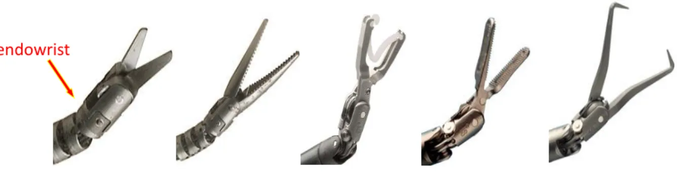
Fig 1.11 shows various types of instruments of Da Vinci. In the shaft end of the instrument is the endowrist, where is considered have most features. Therefore, we will recognize the instrument to represent their positions in the image. In particular, consider that surface of the endowrist is lack of feature points such as corners, we would use spiking neural network to extract the contour and the texture as the features for recognition. Thus the influence of the lack of features can be efficiently reduced.

Since the tool ends of surgical instrument are almost made of metal material, the influence of light change would be even severe and the color on the surface would also change dramatically. For this problem, the edge feature extraction of spiking neural network would less be affected. We can also consider the learning method to train the data of some extreme conditions.

Finally, for the size change problem caused by rotation and displacements of tools can also be solved by training of the artificial neural network. We can let the neural network learn about most of appearances of an instrument to achieve robust tracking. Though it needs great amount of training samples, it can rapidly complete training process because of feedforward learning manner. In this thesis, we want to develop a method to let the endoscopic robot track multiple instruments and provide stable image to the surgeons.

Fig. 1.11 Robotized surgical instruments of Da Vinci system[27].

10

1.5 System Overview

Fig. 1.12 shows the proposed system architecture. The system contains three main parts. The first part is the endoscopic robot which is comprised of a camera holder and an endoscope. The camera holder is responsible for holding endoscope, and the endoscope is for providing the surgical image in the body cavity.

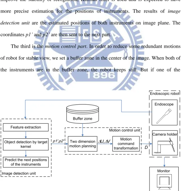
The second is an image detection part. It will firstly extract the features from the surgical image. The positions of both instruments can then be calculated through the selective target kernels which were generated in pre-operation stage. In order to improve the stability of recognition, Kalman filter is used and is expected to have more precise estimation for the positions of instruments. The results of image detection unit are the estimated positions of both instruments on image plane. The coordinates p1’ and p2’ are then sent to the next part.

The third is the motion control part. In order to reduce some redundant motions of robot for stable view, we set a buffer zone in the center of the image. When both of the instruments are in the buffer zone, the robot keeps still. But if one of the

Fig. 1.12 System architecture.

Feature extraction

Predict the next positions of the instruments Buffer zone Two dimension motion planning Motion command transformation Camera holder Endoscopic robot Endoscope Monitor Image detection unit

Motion control unit

V U

 ,

D

Object detection by target kernel

11

instruments is out of the buffer zone, the motion control unit would give the robot motion command. The robot will adjust the pose of endoscope until both of the instruments are back to the buffer zone.

The details are described as follows in the rest of the thesis. Chapter 2 shows the laparoscopic instrument detection. Chapter 3 describes the method of motion control. Chapter 4 shows the experimental results. Chapter 5 is the conclusions of thesis and the future works.

12

Chapter 2 Laparoscopic Instrument Detection

2.1 Proposed Instrument Detection Architecture

In this work, the vision-based instrument tracking task is divided into two main procedures: object recognition and feature tracking. We suggest a novel algorithm to track surgical instrument by using natural features. The algorithm estimates the type of instrument and target position simultaneously. The whole tracking algorithm features a combination of spiking neural network and Kalman filter[28]. The spiking neural network is designed to recognize the instrument tip and the Kalman filter is responsible for robust tracking of multiple instruments.

In the following, we will briefly describe the spiking neural network and its learning process. After network learning, the trained target kernel is used to recognize and localize the instrument in the image frame. The neuro-based tracking system is summarized in Fig. 2.1. It contains three main parts. The first part is to extract the features from input images; the second part uses the trained target kernel to recognize the instrument around the predicted position, which is estimated by the Kalman filter; and the third part aims to update the state of Kalman filter by the measurement in part 2, and predict the next possible position target. The process will be executed the three units repeatedly as long as new images are acquired. The Kalman filter predicts the position of the instruments such that the detection(searching) area can be dramatically reduced. The system can thus achieve efficient and robust tracking of in-vivo surgical instruments.

2.2Model of Spiking Neural Network

We use the same layered architecture to that of SpikeNET. The model consists of three layers and each layer comes to approach the biological visual system. Since the

13

Fig. 2.1 Image tracking algorithm.

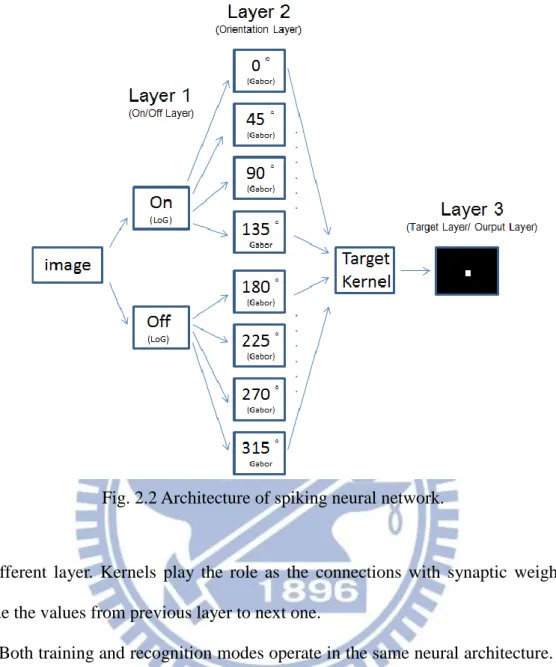
different application from SpikeNET, there is only single output layer in the network. We redraw the model in our manner as in Fig. 2.2. The first layer occurs in ON/OFF pairs that represents the retina. The second layer occurs in a set of eight that mimics the visual cortex(V1) to select the lines in different orientation. The third layer is the output to decide the recognition result which corresponds to IT in biological visual system. Between each layer, there are specific kernels to define the prefer stimulus for

LoG filter Gabor filter

Find the target position in the region around the predicted position

Kalman filter prediciton

Target position p Estimated target position p’ Features extraction Object detection Rank classification according to the intensity of each neuron

Rank order coding

Measurement update Predict the next position of the

instrument Image frames Extend the search region if the instrument is not found The target is detected or the image

has completely scanned

Yes No

14

Fig. 2.2 Architecture of spiking neural network.

the efferent layer. Kernels play the role as the connections with synaptic weight to decide the values from previous layer to next one.

Both training and recognition modes operate in the same neural architecture. But there are still differences during the processing. The first difference is the utilization of the kernel between the second layer and the third layer. When in training mode, the kernel is initialized as an empty array for learning. But in recognition mode, the kernel has completed learning and plays as the synaptic weight to decide the recognition result. For the reason, it is termed target kernel. The second difference is the size of input images. Since the size of target kernel is same as the sample images, the inputs for training should keep in same dimension. However, in recognition process, the size of input images can be different but should greater than or equal to the target kernel. The kernels of each layer are discussed in more detail in the

15 following.

2.2.1 The First Layer of the Network

The purpose of the first layer is to extract edge features. SpikeNET uses difference of Gaussian (doG) as the selective kernel. doG is the second spatial derivative that it is sensitive to edges. And it obtains zero response when the image changes linearly. In our work, we use the use Laplacian of Gaussian(LoG)[29] filter which has the same approximation with doG. The definition of LoG is expressed as the equation such that:

     _      ₄ 2 ₂2 2 ₂2 LoG 2 v u 2 v u 1 1 1 v u W     exp ] [ ) ( ) , ( (2.1)

where (u, v) is the position of the element in LoG array. σ is a the parameter to affect the smoothing when applied. When σ is a large value, the edges after filtering become smoother and less noise remind. η is the parameter to decide the LoG to be ON-center or OFF-center kernel. Fig 2.3(a) shows the 15×15 ON kernel, in whichη is an even number. For the OFF kernel, η becomes an odd number. Fig. 2.3(b) shows the OFF kernel which is reverse to (a).

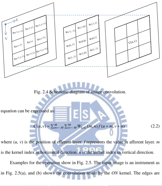
The input image will convolve with the kernels for the edge extraction. In the process of convolution, ON/OFF kernels plays the role as masks to filter out the proper edges from the input image. Suppose the kernels are in size of (2M+1)×(2M+1), where M is an integer. Fig 2.4 shows the schematic diagram and the

(a)ON kernel (b) OFF kernel Fig. 2.3 LoG kernels.

16

Fig. 2.4 Schematic diagram of image convolution.

equation can be expressed as:

     M_{ } M m Mn MWLoG m n f u mv n v u C( , ) ( , ) ( , ) (2.2)

where (u, v) is the position of efferent layer. f represents the value in afferent layer. m is the kernel index in horizontal direction. n is the kernel index in vertical direction.

Examples for the operation show in Fig. 2.5. The input image is an instrument as in Fig. 2.5(a), and (b) shows the convolution result by the ON kernel. The edges are

(a)input image (b)result using ON kernel (c) result using OFF kernel Fig. 2.5 LoG kernel operation.

17

enhanced as bright line that responds to the patterns with positive center and negative surround. Fig. 2.5(c) is the result by OFF kernel that emphasizes different edge features. Results show the output figures keep the same size with the input image.

2.2.2The Second Layer of the Network

The second layer aims to extract texture features. Since texture contains directionality, we use the Gabor filter[30] for line selection in specific angle. The filtering is also the convolution process the same as in first layer but by using the Gabor kernel. Orientation of the kernel can be easily determined depend on our requirement. The equation of Gabor kernel is defined by:

      _                v u u W_Gabor cos 2 2 exp ₂ 2 2 2 (2.3)   sin cos v u u  (2.4)   cos sin v u v  (2.5)

where λ is the wavelength. φ is the phase offset.γ is the spatial aspect ratio that specifies the shape of ellipticity in Gabor function. θ is the orientation setting. The same as SpikeNET, we use orientation layers in a set of eight at 45º rotations. By (2.3)~(2.5), the kernels can be derived that is shown in Fig 2.6. Each kernel has the same value ofλ, φ andγ, only θ changes depending on the requirement of user.

(a)0° (b) 45° (c) 90° (d) 135° (a)180° (b) 225° (c) 270° (d) 315° Fig. 2.6 Gabor kernels.

18

We go on to project the spikes from the first layer to the second layer by Gabor filters. Fig 2.7 shows the oriented edge selection from Fig. 2.5(b). Fig. 2.7(a) is the 0° Gabor kernel convolution. Only the edges in vertical detection are selective and pass through the filter. Fig. 2.7(b) shows the result of 45° Gabor filter. The edges in more like 45° are brighter than others. Fig. 2.7(c) shows the case to find the horizontal edges. Therefore, through the operation, we can derive all the eight different edge figures. All the neuron layers in layer two are also the same size to the input image.

2.2.3Network Learning

The purpose of network learning is to find a proper kernel that can decide the recognition result accurately in the output layer. It locates between layer 2 and layer 3 and is initialized as an empty array with the same size as the sample image prepared for the training process.

(a)0°filtering (b)45°filtering (c)90°filtering (c)135°filtering

(a)180°filtering (b)225°filtering (c)270°filtering (c)315°filtering Fig. 2.7 Gabor kernel operation

19

The learning procedure of the spiking neural network is shown in Fig. 2.8. The input image propagates through the network first processed by LoG and Gabor convolution. Then the produced eight figures in the second layer should merge into a single figure and then transfer to spike latency according to the activation of each neuron. The transformation mechanism is termed the rank-order-coding[32] which is developed by Thorp et al.

For the implementation of rank-order-coding, we need to classify neurons into different ranks and decide their firing order. Once the firing order is decided, the variance of synaptic weight can be derived such that:

J n m w n m r( , ) ) , (    , (2.6)

where m is the kernel index in horizontal direction. n is the kernel index in the vertical direction. β(0,1) and r(m,n) is the firing order of neuron (m,n) in the merged pattern. J is the number of training cases of an instrument. The division operation is to combine multiple kernels to a single target kernel by averaging them.

Fig. 2.8 Training of the spiking neural network. Input an image

Use Laplacian of Gaussian(LoG) to extract the edge feature

Use Gabor filter to update texture features

Rank order coding

Update target kernel

Rank classification according to the intensity of each neuron

20

Fig.2.9 shows the process of target kernel generation. Orientation patterns in the second layer are summed to single figure. In the merged pattern are texture and edge features belong to the recognized target. Suppose the size of each layer is in (2M+1)× (2N+1), where M and N are integers. The target kernel will generate in the same dimension and plays the role as the synaptic weight from the merged pattern to the center neuron of the third layer.

Since the training is a feed-forward procedure, the synaptic weight will be trained when all the prepared image samples have been used in the training process. Each synaptic weight will converge to a value depending on the mean rank of each input. After training, the synaptic weights become constants and can be used as a kernel to recognize a specific target.

2.2.4 Object Recognition

In execution of image tracking, LoG and Gabor convolution are processed for the acquired image the same as that in the network learning stage. The firing order of neurons is estimated accordingly. As usual, we should implement the rank-order-coding directly after feature extraction. However, an improving scheme is proposed in this thesis to be added before the rank-order-coding. The idea is that if the

Fig. 2.9 The schematic diagram of target kernel generation.

(M,N)

Target kernel The third layer (m,n)

The second layer Merged figure (m’,n’)

21

environmental background is complex in the imagery, the target neurons might be inhibited and results in misclassifications. We will describe this part in more detail in Section 2.3.

After the feature extraction, the instrument position will be found by using the target kernel to compute output values of layer 3 around the predicted position. Fig 2.10 shows the schematic diagram of the computation process. Suppose the size of target kernel is (2M+1)×(2N+1), where M and N are integers. The size of the input image is LI×WI, where LI represents the length in horizontal direction and WI is the

width in vertical direction. Since the input image should be greater than or equal to the target kernel, the output value of the third layer can be computed by the expression bellow:                M L 1 M u N W 1 N v M M m N N n n v m u r I I n m w v u A( , )



( , ) ( , ) , (2.7) where LI≧(2M+1) and WI≧(2N+1). (u,v) represents the neural position in the third

layer. w(m,n) is the value of element (m,n) in target kernel. r(u+m,v+n) is the firing order of the neuron (u+m,v+n) of the merged pattern. Finally, the neuron will fire if the value is equal or greater than the threshold:

h

T v u

A( , ) , (2.8)

Fig. 2.10 The process of the recognition value in output layer.

(u,v)

Target kernel

The third layer

The second layer Merged figure

Predicted

22

where Th is the threshold. This procedure of spiking neural network is called

integrate-and-fire [32].

In spiking neural networks, rank-order-coding plays a key role in object recognition. Every object mapped to the network will produce different neural sequences and firing order. So the target object will match the training data only when the neuron fire sequences belong to in a particular order.

Fig. 2.11 shows the example of rank order scheme for recognition. Suppose activation of the neurons is B>A>C>D>E. If β is 0.7, by the rank-order-coding, spike latency of A~E would be (0.71, 0.70, 0.72, 0.73, 0.74). If the neurons of the image for recognition is in the same order and the values of A~E are (4,5,3,2,1). The output value would reach the maximum: 4×0.71+5×0.70+3×0.72+2×0.73+1×0.74=10.1961. But if the input image is in the order A>B>C>D>E, the output value will be 9.8961. Other arrangements would be even lower. Therefore we can set the threshold about 10 for recognition in this case.

Through the rank-order-coding scheme, the trained kernel will be very unique to the specific appearance of the target. But an instrument has different appearances such as change in size and rotation. The adopted strategy is to average the kernels for all the conditions described in (2.6). In this way, the universal kernel can recognize most of the condition s but it loses the uniqueness at the same time. And it

Fig. 2.11 Rank-order-coding scheme.

layer 3 layer 2 intensity A B C D E

23

will be affected by noise more easily. To keep advantage of the recognition capability, the training samples should be as less as possible. Furthermore, the suitable threshold for filtering is also an important factor for a successful recognition.

Once any neuron fires in layer 3, it implies that the object matches the target. The firing neuron will appear at the center point of this object in layer 3. If the instrument has not been detected, then the search region would extend. This process will repeat until the instrument is found or the neural map has completely scanned. If the instrument is successfully detected, its coordinate p will be sent to the next step. Otherwise, p will maintain the previous value for the condition that the instrument is temporarily occluded.

2.3 Object Recognition under Complex Environment

During surgical operation, the effluence of blood and body fluid from tissue occurs frequently. Luster on the organ and tissue become brighter and there are reflections of lighting appear on the fluid. Edges of these reflections are always more intense than the others. By the spiking neural network algorithm, the neurons with highest intensity will fire first. Therefore, the reflections will greatly affect the recognition result. In the following, we will describe the rank order classification and the improved method to reduce the impact of reflection.

As we know, the range of the grayscale image is from 0 to 255. A simple way to decide the firing order is to classify the neurons linearly into 256 ranks depending on their intensity. Fig. 2.12 shows the rank classification. By the known rank level, firing order of each neuron can be defined as:

firing order=255-rank , (2.9)

24 255 will be zero. When firing order rj is 0, j

r

 will reach maximum by the equation

(2.7). It means the neurons firing first have the most contribution to the integration in layer 3. However, because the contribution of each neuron decreases exponentially (Fig. 2.13), only the neurons which fire first will demonstrate the integrated result in layer 3. If the most activated neurons come from the background noise, the tracking performance will be seriously degraded.

Since the intensity of the features in the second layer is greater than the mean value of the image after extraction, we can enhance the firing order of these neurons whose activation are higher than the average. Therefore, the integration of our

Fig. 2.12 Rank classification.

Fig. 2.13 Neural contribution in equation (2.7).

0 50 100 150 200 250 0 0.2 0.4 0.6 0.8 1 j r



firing order rj 0 50 100 150 200 250 0 50 100 150 200 250

activated level of a neuron

ra

n

k

activation of the neuron

ran

25

target can be improved in the third layer. Through the analysis, we suggest to change the rank classification scheme to another type of function such as a sigmoid function. The function is depicted as the solid line in Fig. 2.12 and can be expressed such that:

)) ( exp( ) ( d g 1 G g S s      _, (2.10) where S is the rank and g is the activity of the neuron in layer 2. α is an constant to decide the degree of curvature of the function curve. Gs is a scale depends on the

maximum rank number. In our case, Gs is 255. d is the mean value of the neural map

and it will change depending on each frame. By equation (2.10), the neurons in rank 200 will be upgraded to 230, the firing order is therefore improved. The neurons below rank 100 is downgraded, it will not influence the value layer 3 according to the exponential function.

The proposed classification is adjustable depending on the mean value of the image. The function curve will shift at each frame to achieve suitable firing order adjustment. As we know, the intensity of the extracted features is greater than the mean value. If the input image becomes darker due to the lighting of endoscope, the average value will decrease. The center of sigmoid curve will shift to left according to d in (2.10). Through the adjustment of the function, the firing order of the neurons belong to the features will keep enhanced. For the case of brighter image, the firing order of the neurons which belong to the features can also derive the suitable adjustment through the same process. In this way, it can achieve stable recognition even the luminance changes due to the moving of endoscope during surgery.

We take a snapshot from an in-vivo video of laparoscopic surgery as an example shown in Fig 2.14(a) [34]. Suppose that our target is the right instrument in the image. After this image frame is processed by LoG and Gabor convolutions, the contribution of the neurons from the right instrument will be inhibited by the exponential function

26 (a)

(b) (c) (d) Fig. 2.14 Image tracking under complex background.

in the calculation the rank-order-coding as shown in Fig 2.14(b). With the new classification method, the contribution of the neurons is shown in Fig. 2.14(c). From this image, one can find the contribution of the neurons from the right instrument is much improved. As shown in Fig. 2.14(d), the integrated values in layer 3 will exceed the threshold and fire spikes, which will appear in the center of the right instrument.

With the new classification method, the neurons still maintain a certain firing order, but the firing priority of target neurons is upgraded. This scheme reserves property of rank-order-coding and improve the object detection under complex background.

2.4 Kalman Filter Design

Kalman filter is a recursive estimator based on linear systems [28]. It is efficient for solving numerical engineering problems. The application of Kalman filter has two The right instrument The left instrument

27

classes. The first one as the name is filter for smoothing data sets. The second class is the prediction.

In our study, we use Kalman filter to predict the positions of instruments in the images. We expect the prediction to help to make the image tracking more efficiently through recognizing the instruments surrounding a smaller area of the predicted position. Since the critical time in our algorithm is at the recognition process, Kalman filter would help to efficiently reduce much of redundant computation. In addition, Kalman filter can filter out the unexpected recognition error. It is helpful to stabilize the recognition result for robust tracking. A useful property also refers to that Kalman filter can track the target even encountering the temporary occlusion. For these reasons, we will combine the spiking neural network with Kalman filter for the instrument tracking in the endoscopic image sequences.

The main process of Kalman filter contains prediction step and correction step. Prediction is to estimate the next possible position before the next endoscopic image come in. Correction is to attain measurement by the detected position. In our algorithm, Kalman filter plays a role as a tracker and spiking neural network is the detector. In order to achieve the better performance, Kalman filter will predict the instrument not only by position but also by velocity. The details of computation are described as below:

We first define xˆ_k1 be the posteriori state at instant k-1 and xˆ_k be the predicted state at instant k. The state of the Kalman filter includes the information of instrument position and velocity. The posteriori state can thus define as

T 1 -k 1 -k 1 -k 1 k 1 k X Y dX dY

xˆ _ [ _ ] , where Xk-1 and Yk-1 are the coordinate of the instrument

in x and y axis while dXk-1 and dYk-1 are the displacements. To predict the first

28 state xˆ_k can be estimated such that:

xˆ_kFxˆ_k1Be_k1 , (2.11) where F is a transition matrix applied to posteriori state xˆ_k1, B is a control input

matrix applied to the control vector e_k1. In order to simplify the state estimation, we

assume that there is no control input, so e_k1 will be a zero matrix. We also assume

that the instruments move in a constant speed such that the displacement d ˆX_k=dX_k1

and d ˆY_k=dY_k1. The predicted position (Xˆk,



k

Yˆ ) can be (X_k1dX_k1,Y_k1dY_k1). The overall predicted state becomes:

                                               1 1 1 1 1 0 0 0 0 1 0 0 1 0 1 0 0 1 0 1 ˆ ˆ ˆ ˆ k k k k k k k k dY dX Y X Y d X d Y X .

We rewrite equation (2.11) as:

1 ˆ ˆ _{ } k k Fx x , (2.12)

By equation (2.12), the matrix F can be determined. The first predicted position p’ can also be derived. Then the priori estimate covariance can be computed such that:

Q F P F Pk  k k kT   1 , (2.13)

where Q is the process noise covariance matrix, and Pk-1 is equal to identity matrix I4.

The next important step is to apply the measurement update t of Kalman filter namely the correction. The first task of the correction is to compute the Kalman gain:

1 ) (    _ P H H P H R K_{k k k}T _{k k k}T , (2.14)

29

where H is a measurement matrix. R is the measurement noise covariance matrix. Then by the recognition process around predicted position p’, we can derive a detected position p by spiking neural network. Then we rewrite the coordinate p as matrixz to generate the posteriori state _k xˆ , such as: k

) ˆ ( ˆ ˆ _ _{ }  k k k k k k x K z H x x , (2.15)

And the posteriori error covariance P_k is expressed as follow:





 _{k k k}

k I K H P

P ( ) _, (2.16)

In some cases, the noise covariance matrixes Q and R, and the measurement matrix H might be time varying. We assume them as constants in this design for simplification. And in our work, we set Q and R the 4×4 identical matrix with a very small scale and H the I4.

Fig. 2.15 summarizes the proposed tracking algorithm using Kalman filter. The prediction of the two instruments should be estimated separately by two Kalman filters. Therefore, we create two Kalman filters and initialize the parameters to predict the possible positions for the first frame by e (2.12) and (2.13). The system then starts to recognize the instrument around the predicted positions by spiking neural network. The derived measurement positions p1 and p2 imply the coordinates of the left and the right instrument respectively. In order to predict the next position for next frame, we let zk be the transpose matrix of p1. Through the correction step by (2.14)~(2.16),

the state of the left instrument can finish update. And the next possible position of the left instrument p1’ can be estimated by (2.12) and (2.13). The predicted position of the right instrument p2’ can be derived by the same process.

30

Fig. 2.15 Instrument tracking using Kalman filter.

Both of p1’ and p2’ will be sent to the motion controller to transfer to the robot commands Du and Dv, which implies the displacements in horizontal and vertical

direction respectively. In the same time, the predicted positions p1’ and p2’ will be reserved for the reduction of searching area in the next frame. In this way, Kalman filter can help to achieve efficiently tracking in robotic endoscope system.

However, if the instrument has not been recognized before the correction step, the measurement matrix zk will stay as the previous value in our work. In this way, the

prediction will keep moving on for a while and go back to the position that loss detection. Therefore, if temporary occlusion occurs during the process that the instrument pierce the tissue, the system can soon find the instrument along the moving direction. But if the instrument is vanish for a period, the system will detect around zk

Measurement update

Prediction

Controller Endoscopic

Robot Find the instruments position p1and

p2 in the region around p1’ and p2' respectively Predicted position p1' and p2' Motion command Du and Dv zk=p1T

(1)Compute the Kalman Gain (2)Update the estimate via zk

(3)Update the error covariance

1 T k k k T k k k P H H P H R K   (   ) ) ˆ ( ˆ ˆ _ _{ }  k k k k k k x K z H x x    k k k k I K H P P ( )

(1)Project the state ahead

(2)Project the error covariance ahead

k 1 k F x xˆ  ˆ Q F P F Pk 1  k1 k kT1   Image frame zk=p2T Kalman filter

31

and extent the searching area until the instrument is rediscovered or the image is completely scanned. Therefore, for the condition that surgeon changes the instrument, the tracking will soon restart from the border of the image.

32

Chapter 3 Image Tracking System

After instrument recognition, the system can track the instruments in an image sequence. The next step is to combine the robot control with image recognition. The purpose here is to let endoscope provide stable image when robot track the instruments. In the following, we describe proposed buffer zone design for the issue in Section 3.1. Section 3.2 tells about the workflow of image tracking. We further describe motion control by using buffer zone in Section 3.3.

3.1 Buffer Zone Design

By knowing the location of both instruments, the camera can track them by using feedback controllers. However, it would make surgeons dizzy if the tracking controller is sensitive to the movement of the instruments in the image frame. In order to solve this problem, we propose to set an area termed buffer zone in the center of the image[33]. Buffer zone offers a suitable buffer space to avoid excessive control actions and thus the movement of the camera and thus maintain a stable imagery. Surgeons can therefore operate the instruments with a series of motion without moving camera. The schematic diagram of buffer zone is depicted in Fig. 3.1.

Fig. 3.1 Schematic diagram of buffer zone.

33

We will use the ratio between size of buffer zone and image plane to describe the choices for buffer zone, such that:

, (3.1)

where LI and WI denote the length and width of image frame respectively. And LB and

WB are the length and width of buffer zone. The parameters of equation (3.1) are

depicted in Fig. 3.2. To get larger movable range for instruments, we want the buffer zone to have larger size, but the tracking performance will become worse relatively. The factor to affect tracking performance is the area outside the buffer zone. If the area is large, it will have more space to get the tracking command. In determining the size of the buffer zone, it is a trade-off between reducing camera movement and improving tracking performance.

3.2Workflow of image tracking implementation

Since surgeons use two of the instruments in the operation to guide the robot into the required location, the system starts the robotic control only when both of the instruments are detected. Fig. 3.3 shows the flow chart of the proposed image tracking design. When none of the instruments appears or only one of them is detected, the system will keep detecting without moving. Once both of them have been detected, which implies that the surgeons are ready to implement the operation, the system will start to track the instruments with motion control estimation.

Fig. 3.2 The ratio of buffer zone. L_B L_I W_B W_I I B I B W W L L Rt 

34

Fig. 3.3 The flow chart of motion control.

We divide the tracking procedure into two fundamental modes in the camera holder operation. One is the operation mode, and another is the tracking mode. Fig. 3.4 shows the working principle of two operation modes of laparoscopic instruments during the surgery. When both of the instruments are inside the buffer zone, system enters to operation mode. In this mode, surgeons operate the instruments with a series of tool motion without introducing camera motion. The camera view stands still. It is desirable for doctors to concentrate on operation. But if one of the instruments moves outside the buffer zone, the system will switch to tracking mode and control the robot

Fig. 3.4 Two operation modes of laparoscopic instruments tracking. Instrument detection

Only one of the instruments is out of buffer zone Both of the instruments

are detected

Order the the

endoscopic robot to track the instruments yes

Images

no

no

Estimate the displacement of robot command yes

Operation

Mode

Tracking

Mode

One of the instruments is out of buffer zone.

Both of the instruments are in buffer zone or both of them are out of buffer zone

35

move to the instrument beyond the buffer zone. The robot will keep moving until both of the instruments are back to the buffer zone. But if both of the instruments are out of buffer zone during tracking, the robot will keep also still by considering the safety problem. When the surgeons need to change the instruments during operation, the system again keeps detecting without control. Therefore, it is safe in the whole process of surgery. And in this way, the system can achieve two dimensional tracking.

Furthermore, we expand the concept of buffer zone to the third (depth) dimension tracking. In doing so, we set a range of the Euclidean distance between two instruments as a measure of the distance between the camera lens and instruments. This depth should be kept a proper value and maintain stable during the surgery. Suppose the Euclidean distance between the instruments is Ed. If Ed is a small value, it

is likely that the surgeon is operating at a delicate part in body cavity, but the camera shot is too far away from the instruments. In this situation, it is desirable for the surgeon if he/she wants to zoom in the camera to watch a clearer view. In contrast, if Ed is too large or both instruments cannot be contained in a single image, it means that

the camera is too close to the instruments. Thus the endoscopic robot would lose tracking easily. It would be helpful if the endoscopic robot zoom out autonomously in this condition. Therefore, by evaluating the magnitude Ed, the robot can control the

third dimension. And the controller would autonomously adjust the robot’s configuration along the third dimension to make Ed to the suitable value. It also

implies that the robot would keep an appropriate distance from camera shot to the instruments.

We hardly have better information about image depth by using monocular camera. Fortunately, the parameter Ed we proposed can help us to realize the

instruments roughly in the third dimension. However, it would be unstable in specific condition. Fig. 3.5 shows the condition where it is not applicable by considering Ed

36

(a) (b)

Fig. 3.5 Specific condition that would be misjudged. (a)Top view, (b)Side view.

merely. The robot does not know actually how deep the two instruments are, but it only knows Ed is very small and out of the range. Therefore, the robot will zoom in

the camera continuously and touch the right instrument. It will lose its stability in the end. Therefore, the motion control of zoom in/out is not added in the system currently.

3.3 Motion Control of Robotic Arm

Fig. 3.6 shows the architecture of robot control. System detects the instruments and estimates the predictions p1’ and p2’ for the left and the right instrument respectively. p1’ and p2’ will send to the comparators to compare with boundaries of buffer zone in both horizontal and vertical directions. Suppose u1 and u2 are the horizontal (U) component of p1’ and p2’, uup and udn are upper bound and lower

bound of buffer zone in horizontal direction. Once u1 or u2 is out of the boundary, the comparator starts to estimate the deviation ΔU between the instrument and the buffer zone:          dn dn up up u u for u u u u for u u U , (3.2)

The deviation in vertical (V) direction can be estimated in the same way:

         dn dn up up v v for v v v v for v v V , (3.3) Ed Ed

37 Controller Horizontal boundaries of buffer zone Detect the instrument positions p1,p2 Vertical boundaries of buffer zone Predict the instrument positions p1’=(u1,v1) p2'=(u2,v2) Endoscopic robot p1,p2 ΔU ΔV Du,Dv u1,u2 v1,v2 comparator comparator uup ,udn vup ,vdn

Image detection unit

Motion control unit Fig. 3.6 Control architecture of surgical instrument tracking.

Fig. 3.7 Boundaries of buffer zone.

where (u,v) denotes the instrument position which is out of the buffer zone. And the corresponding boundaries lines are illustrated in Fig. 3.7.

The controller then transfers the deviationsΔU and ΔV into robot commands. The motion command in U and V directions are defined as:

U G D_u  _u , (3.4) V G D_v  _v _{, (3.5)}

38

where D and _u D are the displacements that the robot have to move in U and V _v

directions. G and _{u G are controller gains, which can be decide as arbitrary v} numbers in positive. The negative signs in (3.4) and (3.5) are because the moving directions are opposite to image coordinate. Therefore, the camera holder will move with displacements D and _u D in U and V directions untilΔU andΔV reduce to _v zero. Through this error correction, both of the instruments will back inside the buffer zone, and the system return to operation mode. In this way, the endoscopic robot can achieve two dimensional tracking.

39

Chapter 4 Experimental Results

In this section, we implement our proposed algorithm and show experimental results of instrument tracking. In Section 4.1, we verify the tracking algorithm by using in-vivo endoscopic video. In Section 4.2, we have another experiment to combine image recognition and robot control to achieve an autonomous endoscopic system. And in Section 4.3, we have some discussions of the experiments. The analysis is expected to have better results and practicality in real surgery.

4.1 Experiment by Using In-vivo Endoscopic Video

A video from IRCAD [34] was used to verify the proposed algorithm to track surgical instruments in the actual laparoscopic surgery. As shown in Fig. 4.1, in the video there are two instruments in opposite directions. In the image sequences, the instruments change their poses and deform on the tips.

4.1.1 Data Training of the Instruments

To train the target kernel of each instrument, the part of the instrument wrist is selected as feature to recognize. Six training samples of the right instrument were

40

used as shown in Fig. 4.2. The training process is depicted in Fig. 4.3. After the training process of each individual sample image, 6 target kernels were generated. These 6 target kernels are merged to a target kernel according to (2.6). The target kernel of the left instrument is also trained in the similar way, however, only 4 training samples were used in this case as shown in Fig.4.4.

Fig. 4.2 Training samples of the right instrument.

Fig. 4.3 Training process of the right instrument.

41

4.1.2 Instruments Recognition by Using Video

We then used these two target kernels together with the Kalman filter to track the instruments in the video. The firing neurons are tracked in the center of the instrument. The position of the instruments can thus be determined. Fig 4.5 shows a tracking result of the test video under the condition of light variation. The right instrument still can be tracked properly in this case. Fig.4.6 shows the tracking condition when the left instrument has size variation in the image sequence. It can be seen also that the problem of rotation and deformation of the instrument in the imagery are solved by

Fig. 4.5 Lighting variation condition.

42

spiking neural network. The tracking results show the robustness of the tracking design. In the experiments, the test video contains totally 897 frames. Table 4.1 shows that the recognition rate of the right instrument is 91.9% and that of the left one is 99.1%. The tracking system was implemented on an i3-330M (2.13GHz) personal computer. The computational speed is 4.8 frames per second(fps) when the Kalman filter has not been used. It improves to 8.0 fps with the assistance of the Kalman filter.

4.2 Experiment of Visual Servo by Endoscopic Robot

The purpose of this experiment is to combine the image recognition with robot control to have an autonomous tracking system. We will use two robotic instruments from Da Vinci system in this experiment. We will hold both instruments by hands and move the instruments on image plane. The scenario is to simulate the surgeons operate the De Vinci system in MIS.

4.2.1 Experimental Setup

Fig 4.7 shows the hardware architecture that is comprised of image devises and the Huatuo robot. Image devices provides surgical image to the robot, and Huatuo robot[34] controls the motion of robot arm to track surgical instruments.

Table 4.1 Recognition result of in-vivo endoscopic video.

Testing frame Detected frame Recognition rate Kernel 1 (right instrument) 897 824 91.9% Kernel 2 (left instrument) 897 889 99.1%