所得分配、所得不均度與所得成長

(1)

Income Distribution and Inequality

Abstract

The distribution of incomes is composed of two kinds of fractal distributions rather than symmetric normal distributions. Income distribution is less dispersed in the higher income group than it is in the lower income group. Also, the higher the initial income level is, the lower the variant in both the average annual income growth rate and the standard deviation of the annual income growth rate. Income growth differs from the case of city growth in that income growth delivers Gibrat's law in the lower tail. The attributes of income distributions and the growth process of two groups of countries are dissimilar. Inequality demonstrates one aspect of distribution. We attempt to study income inequality according to the nature of income distribution, which is an approach disregarded by the traditional way. The purpose of this paper is to measure inequality from a different perspective, to investigate the underlying distribution properties, both between and within two groups of nations, and inspect any possible differences between this approach and the traditional method. Various inequality indexes, including Pareto coefficient are used to measure inequality both in the world as a whole and within the two groups of countries. We find that incomes among the lower income group countries generally deviate significantly more than they do in the higher income group. Using Gini to measure the whole blurs the tendency of income inequality to be substantially different between the two groups. Most indexes of the lower income group of all countries have analogous time trends; however, the indexes of the two groups show that the trend is towards significantly opposite directions. In general, the income inequalities of the two groups reveal distinct features in terms of scale, trend, time-series attribute, and the relation to income growth and mean income. The nature of income distribution among the countries of the lower income group is much more similar to that of countries as a whole. The OPEC recession had a reverse effect on the tendency of disparity between developed and developing countries. Data reveals a trend of increased economic polarization between developed and developing countries rather than among countries overall. Analyzing income distribution overall, despite different groups, may overlook some underlying features.

Hsin-Ping Chen Department of Economics National Chengchi University

(2)

1. Introduction

The distribution of country income is neither equal nor symmetric with the mean income: there are many more countries with incomes below the mean income than above it. The distribution is skewed toward right and approximates two types of fractal distributions rather than a single normal one. Numerous works have applied various indexes in studying the features of aggregate inequality in spite of the nature of income distribution. There are different indexes for measuring income inequality including the Gini concentration ratio (Cowell, 1995), Theil's inequality index, the Generalized Entropy measure (Shorroks, 1980) and the Oshima index (Kuznets, 1963; Sen, 1973; Morduch and Sicular, 1996). Both the Gini concentration ratio and Theil inequality index measure the dispersion of income in terms of the divergence to population share. The Oshima index takes the ratio of the top 20 percent average income to the lowest 20 percent average income. Additionally, the coefficient of variance offers a simple means of measuring dispersion.

Milanovic (2002) used the Gini index to calculate the income distribution among individuals around the world, based on household surveys from 91 countries, and found that inequality increased from 1988 to 1993. This increase was driven more by differences in mean incomes between countries than by inequalities within countries. Firebaugh and Glenn (1999) employed a general formula for inequality indexes to study inter-country income inequality. They found that the trend toward rising inequality leveled off from 1960 to 1989, which failed to provide support for the theory of world economic polarization receives. The distribution of income in a country is traditionally assumed to shift from relative equality to inequality and back to greater equality as the country develops.The traditional Kuznets hypothesis (Kuznets, 1955) postulated a nonlinear relationship between a measure of income distribution and the level of economic development (Bulir, 2001). Deininger (1996), making intertemporal and international comparisons, did not find a systematic link between growth and changes in aggregate inequality but does find a strong positive relationship between growth and poverty reduction.

In addition, prior sociological studies of inter-country inequality used world system and dependency perspective to predict increasing cross-nation polarization and thus a rising inter-country inequality. The polarization theorists place the greatest emphasis on the mechanisms by which nations at the top become richer at the expense of nations at the bottom.(Korzeniewicz and Moran, 1997) Income inequalities result from economic growth differentials that occurred between different cities over time. The theoretical literature differs on whether increased integration promotes or reduces income disparities. Urban disparities were cyclical -- decreasing during strong growth

(3)

and increasing in slower growth years. The positive linear relationship between levels of national income and urban disparities has implications for economic polarization (McCarthy, 2000). Yorukoglu and Mehmet (2002) studied the relationship between population density and income inequality across countries and found population density and income inequality are closely linked.

The fractal distribution can be transformed into Pareto distribution and the corresponding Pareto coefficient is an indicator of dispersion. The unsymmetrical feature of income distribution and the corresponding Pareto coefficient have not been empirically applied in interpreting the aggregate inequality. The inequality displays one aspect of distribution. We attempt to study income inequality according to the nature of income distribution which is largely ignored in the traditional approach. The purpose of this paper is to measure inequality from a different perspective, to examine world income inequality by taking the view of a skewed and separated income distribution and to investigate the underlying distribution properties between and within two groups of nations, and hopefully to inspect the possible differences that vary from the traditional method. Various formulas for inequality indexes including the proposed Pareto coefficient are measured intertemporally, not only in the world as a whole, but also within two groups of countries. This is to investigate the features of income distribution overall and among groups of countries, and moreover to investigate the questions in previous studies from a different prospective.

2. The indicators of inequality

The general formulas for inequality indexes are as follows:

The Gini coefficient (G)

The Gini coefficient is derived from the Lorenz curve, a cumulative frequency curve that compares the distribution of a specific variable with the uniform distribution that represents equality. It ranges from 0 to 1, reflecting the level of inequalities of the specific variable corresponding to the distribution of population. A value of 0 represents perfect equality and a value of 1 total inequality. The coefficient can be written as

∑

= = − = n j j i j i n i Y Y p p G 1 1 ) / 1 ( µ

,

(1)

where Yi represents income in country i, µ is the world average income, pi: refers to the population share of country i,and n is the number of countries.

The Theil inequality index (J)

The Theil inequality index (1967) is derived from the concept of relative entropy (known as the Kullback-Leibler divergence). It measures the distance between the

(4)

of the specific variable and the population is measured by the corresponding proportion and weighted by the population share. This inequality index is given by

∑

= = = = n i i i n i i i i p y p j p J 1 1 ln ) ln(

,

(2)

2 1 2 1 ) (ln ] ) [ln( '

∑

= = = = n i i i n i i i i p y p j p J

,

(3)

where yi is the income share of country i. This index measures the level of dispersion relative to the distribution of population, which is similar to the Gini coefficient. It can be decomposed into inequality between regions (Jbr ) and

inequality within region (J ). _r

∑

= = m r r r br p j J 1 ln

,

(4)

∑

= _ir _ir r p j J ln

,

(5)

∑

+ =Jbr prJr J

.

(6)

where parameter m refers to the number of subregions, pir represents the population share of country i in the subregion r

.

The Generalized Entropy indicator (GE)

This indicator often called the mean logarithmic deviation, is the transformed Theil inequality index. It is defined as the sum of the log of the world average income relative to the country income, weighted by the country's population share as in the Theil index. The divergence of the specific variable is measured according to its own mean value rather than the population share as in the Theil index.

∑

= = n i i i Y p GE 1 ) ln(µ

(7)

2 1 ] ) [ln( '

∑

= = n i i i Y p GE µ

,

(8)

where the variables are defined as in the previous indicators.

The Oshima index (S ) y

This index is defined as the ratio of the top 20 percent average income (YH)to the lowest 20 percent average income (Y ). It is a rough measure of the divergence of a L

specific variable regardless of the distribution of population.

L H

y Y Y

(5)

Fractal distribution and the Pareto coefficient (β )

The fractal distribution is positively skewed. It has a long tail of high values and consists of an ever larger number of ever smaller values. The general distribution of a fractal system has the power function form; thus, it follows the Pareto distribution:

β − = Ax

x

F( ) ,

(10)

where F(x) is the cumulative distribution function, and the number of observations is at least as large as x. Consequently, the rank for x is inversely proportional to size

x with a constant exponent,β , known as the Pareto coefficient. This coefficient

measures the level of diversification. The plot of log of rank versus log of size approximates a straight line.

) log( )

log( )

log(Rank = A −β Size .

(11)

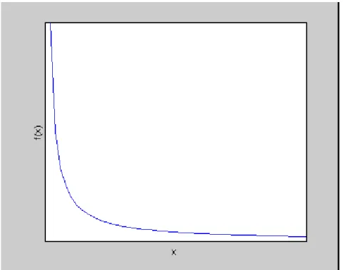
Fractal distribution is defined by the linearity of the power law form. It is characterized by the Pareto coefficient (Chen, 2003). Figure 1 shows an example of fractal distribution. The larger the coefficient, the more evenly distributed are the sizes of x. The distribution follows Zipf's law when the coefficient equals one. Gabaix (1999) stated that an independent growth process leads to Zipf's law. It implies that the probability distribution of the growth process is related to the value of the Pareto coefficient, which measures the level of dispersion.

3. Data and measurement

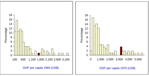
The data of world income is based on the real Gross Domestic Product per capita from the Penn World Table 6.0 for up to 140 countries in a thirty-nine year period (1960~1998). The world income inequality is measured based on various indicators introduced in Section 2. Figure 2 presents the distribution of income. The distribution of income is not symmetrical; it is rather close to two different kinds of fractal distributions. Diagrams of log of rank versus log of income are shown in Figure 3. The kinked point between the lines is getting apparent each year. Countries are classified into two groups according to the income level at the kinked point each year as shown in Figure 3. Group 1 contains nearly the top 16 percent higher income nations and Group 2 contains the remaining 84 percent lower income nations.1 There are strong negative linear correlations of log of rank versus log of income in both groups verified by Meta analysis; consequently, this linearity feature

1_{Nations in Group 1 belong to High-income OECD members except for Singapore, Hong Kong, and}

(6)

characterizes fractal distributions.2 The absolute value of the slope, the Pareto coefficient in Section 2, measures the level of dispersion. Moreover, the slope of line of the lower income group is significantly flatter than that of the higher income group. This is statistically examined by the Paired t test.3 It implies that per capita incomes of the higher income group distributes more evenly than those of the lower income group.

Gibrat’s law suggests that homogeneous growth processes lead the distribution converging into a Zipf pattern as fractal distributions (Gabaix, 1999); thus we inspect the growth feature of income. The average annual income growth rate versus the corresponding initial income is shown in Figure 4; the standard deviation of income growth rate versus initial income is shown in Figure 5. Both the average of and the standard deviation of the annual income growth rate of the higher income group are significantly less dispersed than those of the lower income group. The higher the initial income level, the lower the variant are both the average and the standard deviation of the annual income growth rate. This is statistically examined by Goldfeld-Quandt test which detects the presence of heteroscedasticity (see Table 1). Similarly, the standard deviation of the cross-sectional yearly income growth rate is significantly smaller in the higher income group4.

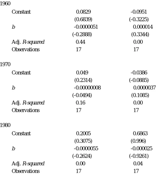
Generalized least squares are applied to regress the average (and the standard deviation) of the annual income growth rate on the initial income. The results overall and by groups are presented in Table 2, 3 and 4. Table 2 shows that the average income growth rate is independent of the initial income and approximates a constant. The standard deviation of the income growth rate is negatively related to the initial income. In Table 3 and Table 4, both the average of and the standard deviation of income growth rate in the two groups are not significantly related to the initial income. In the lower income group, the estimated constants in the regression of average income growth rate are significant in 1970 and 1980; and the estimated

2

Meta analysis tests the hypothesis that the correlation coefficient of log of rank versus log of income in each group is significantly smaller than -0.9 at the 0.01 significance level. The Fisher's Z statistics of Group 1 is -34.36, and the Fisher's Z statistics of Group 2 is -30.01 (Hedges and Olkin,1985; Lipsey and Wilson ,2001; Wolf, 1986).

3_{Paired t test concludes that the estimated Pareto coefficient of the higher income group is}

significantly larger than that of the lower income group at the 0.01 significance level. The test statistics is 23.65.

4_{Meta Analysis is applied to test the value of the correlation coefficient of the log of standard}

deviation of the cross-sectional yearly income growth versus log of income level. We find that the correlation coefficient is significantly smaller than -0.5 at the 0.01 significance level. The Fisher's Z

(7)

constants in the regression of the standard deviation of income growth rate are significant in 1960 and 1970. Both the average of and standard deviation of income growth rate are independent of the initial income in the lower income group. This result verifies Gibrat's law, considering the average Pareto coefficients in the lower income group is 1.07.5 The probability distribution of income growth rate in the lower income group is nearly homogeneous; accordingly, the Pareto coefficient is close to one. Different from the case of city growth, world income growth delivers Gibrat's law in the lower tail. Analyzing income distribution overall, despite group differences, may overlook some underlying features.

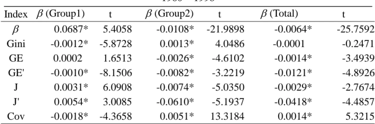
Inequality indexes are measured overall and within groups. The trends of indexes are displayed in Figure 6. In general, income inequality within Group 2 deviates more than that in Group1 except for the Pareto coefficient. Also, measures of inequalities overall are much closer to the measures of Group 2. This may be due to that the number of nations in Group 2 represents 84 percent of the total countries. Results from trend regressions of all indexes are presented in Table 5. In general, Group 2 and the total countries have a similar inequality trend tendency; inequality trends in Group 1 are significantly different from those in Group 2 examined by likelihood ratio test.6

The value of GE indexes, which measures the level of the dispersion of the country income relative to the world average income, has had a diminishing trend since 1976, the year of the OPEC recession, overall and in Group 2.8 The value of J and J’ indexes, which measures the level of dispersion of country income share relative to corresponding population share, has a similar diminishing trend since 1976 overall and in Group 2. Both GE and J indexes show that income distribution is tending to inequality at first and then changes to equality overall and in Group 2. However, income disparity in the higher income group shifts to relative equality first and tends to relative inequality, referring to the measures of Gini and the Pareto coefficient. The turning years in both groups are around 1976. The OPEC recession caused nearly reverse influences on the disparity in both developed and developing countries.

The Gini coefficient measured from the total countries oscillates and does not

5_{Gibrat's law refers to a growth process with common mean and common variance (homogeneity}

growth processes) that generates unity to the Pareto coefficient (Zipf’s laws).

6_{The likelihood ratio test shows that trend lines of the inequality indexes from the two groups of}

countries are significantly different at the 0.01 significance level. (Judge, 1988; Greene, 2000)

(8)

reveal a significant direction of trend. The Gini of Group 1 has a significantly negative trend, while to the contrary, the Gini coefficient of Group 2 has significantly a positive trend. Measuring Gini overall blurs the inequality trends of two substantially different groups. The indexes of all countries and Group 2 have similar trends except for the Gini. Mostly, trends of indexes in the two groups display significantly opposite directions.

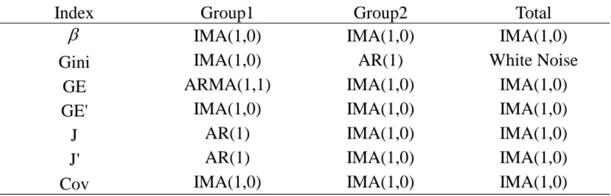
In addition, time-series analysis is applied to test the time-series features of all indexes in the two groups shown in Table 6. We find that the time-series characteristic of the inequality indexes overall is similar to that of Group 2; while the time-series characteristic of Group 1 is much more different. Results from trend regression and time-series analysis indicate that the time-series features of income distributions in the two groups are quite distinct.

Trends of average income and corresponding growth rate are displayed in Figure 7. Trends of population density and corresponding growth rate are shown in Figure 8. The disparity between the higher income group and the lower income group is getting severe with the development of economy overall. The nations at the top become richer relative to the nations at the bottom. The income growth rate of the lower income group vibrates much more than that of the higher income group. Population density of the higher income group is much lower than that of the lower income group; further, the trend of population density of the higher income group grows more slowly than that of the lower income group. Opposite to the dispersion of income growth rate, the growth rate of population density of the higher income group vibrates much more than that of the lower income group. The trend of income inequality within high density, lower income countries is diminishing with the increase of population density; conversely, the income inequality within low density, higher income countries increases slightly.

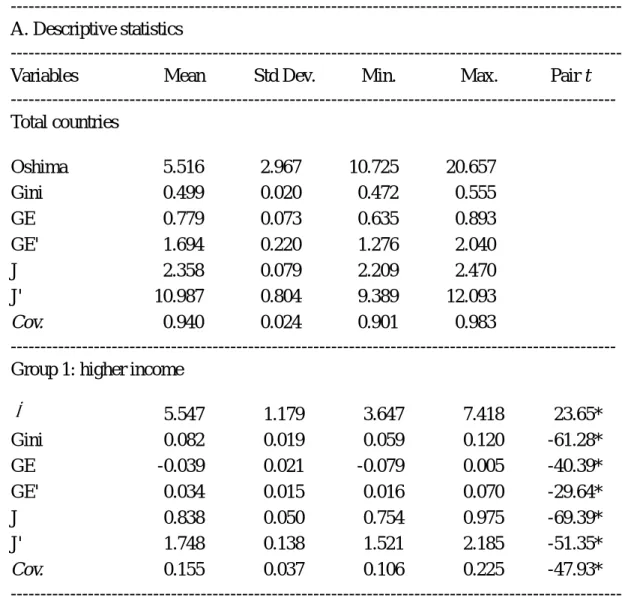
Various indexes rate the scale of inequalities from different aspects. The level of income inequalities measured by all indexes is significantly higher in Group 2 than that in Group 1. This is examined by the Paired t test. The descriptive statistics and the results of the Paired t test are shown in Table 7. The Pareto coefficient (β ) in Figure 3 is significantly larger in Group 1 than in Group 2. All the other inequality indexes are significantly smaller in Group 1 than those in Group 2. This implies that the incomes of lower income countries deviate significantly more than those of the higher income countries. The two groups of countries reveal distinct features in terms of scale and the trend of income inequality. The correlation matrix of all indexes is shown in Table 8. The Pareto coefficient (β ) is strongly negative when correlated to the Gini and the coefficient of variation. GE and J indexes overall and in Group 2 are highly linearly correlated; in Group 1, the relation is trivial

(9)

and insignificant.

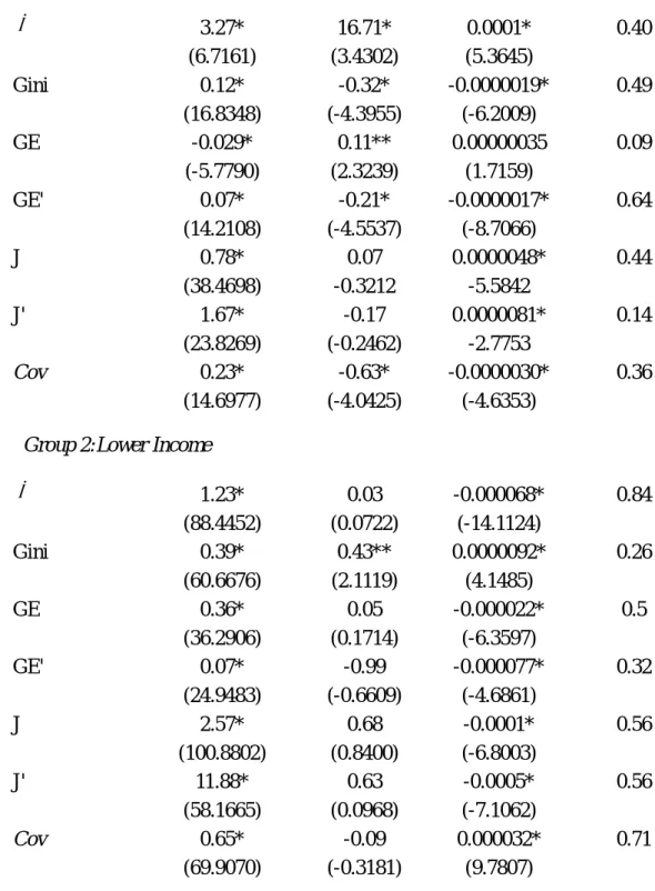
The relation between inequality and growth is examined by the regressions of various inequality indexes on the average income and mean income growth rate. The result is shown in Table 9. In general, the mean income growth rate does not have significant effects on most inequality indexes overall and in Group 2. On the contrary, in Group 1, mean income growth rate has a significant influence on most indexes except J and J’. The average income has a significant effect on almost all indexes in three regressions (Total, Group 1 and Group 2) except for Gini from total nations and GE in Group 1. The direction of the effect of the average income on various inequality indexes in Group 1 is opposite to that in the other two groups. In short, the relation between income growth and inequality in the higher income group demonstrates quite different result overall and in the lower income group. This again verifies that income distributions of the two groups possess distinctive features. There is a positive relationship between the level of economic development and the reduction of inequality except in those higher income countries.

(10)

4. Concluding remarks

The distribution of incomes is not symmetrically normal; rather, it is composed of two different scales of fractal distributions. Accordingly, national incomes are classified into the two groups. Pareto coefficients assessed separately in the two groups are significantly different, and indicate that distribution of per capita incomes are less dispersed in the higher income group than they are in the lower income group. Moreover, the higher is the initial income level, the lower is the variance in both the average of and the standard deviation of income growth rate. Income growth differs from the case of city growth in that income growth delivers Gibrat's law in the lower tail.

In addition to measuring income disparity overall, various inequality indexes are measured separately, for each group, to investigate the nature of income distribution between groups. We find that the overall indexes and those of Group 2 have similar trends. However, changes of inequality in the two groups have significantly opposite directions. Using Gini to measure overall income disparity blurs the tendencies of income inequalities between two substantially different groups. Both the GE and J indexes show that both income distribution overall and that of lower income nations tend initially towards greater inequality and then change, moving towards greater equality. Referring to the Gini and Pareto coefficient measures, income disparity in the higher income group, on the contrary, tends towards greater equality in the beginning and changes towards greater inequality. The year in which the trend reverses in both groups is around 1976, which is the year of OPEC recession. Higher oil prices caused a reversal in the tendencies of income disparity between developed and developing countries. Income inequalities result from economic growth differentials occurring between different countries over time.

Income inequalities within the two groups of nations reveal distinct features in terms of scale, trend, time-series attribute, and the relation to income growth and mean income. The properties of the lower income group are much closer to those of all countries as a whole. The disparity becomes critical between the two groups with the emergence of their divergent economic development and contrasts with the diminishing of inequality within the lower income countries. Increased integration promotes income disparities between groups; however, income disparity within the lower income group falls. There shows a trend of economic polarization between the two groups of countries rather than among countries overall. Our results suggest that measuring income inequality disregarding the nature of income distribution and analyzing income distribution overall despite differences between groups may overlook some underlying features.

(11)

References

Aaberge, R. (2001) Axiomatic Characterization of the Gini Coefficient and Lorenz Curve Orderings. Journal of Economic Theory 101:115-132

Atkinson, A.B. (1976) The Economics of Inequality. Clarendon Press. Oxford

Azzoni, Carlos R. (2001) Economic Growth and Regional Income Inequality in Brazil. The Annals of Regional Science 35:133-152

Bulir, Ales. (2001) Income Inequality: Does Inflation Matter? IMF Staff Papers 48 (1):139-159

Champernowne, D.G. and Cowell, F.A. (1998) Economic Inequality and Income Distribution. Cambridge University Press. Cambridge and New York

Chen, H.P. (2004) Path-Dependent Processes and the Emergence of the Rank Size Rule. The Annals of Regional Science, forthcoming

Chotikapanich, D. (1997) Global and Regional inequality in the Distribution of Income: Estimation with Limited and Incomplete Data. Empirical Economics 22:533-546

Cowell, F.A. (1995) Meqsuring Inequality. Prentice Hall-Harvester. London

Cowell, F.A. and Jenkins, S.P. (1995) How Much Inequality Can We Explain? A Methodology and an Application to the United States. The Economic Journal 105 (March):421-430

Fedorov, Leonid. (2002) Regional Inequality and Regional Polarization in Russia, 1990-1999. World Development 30(3):443-456

Firebaugh, Glenn. (1999) Empirics of World Income Inequality. American Journal of Sociology 104(6):1597-1630

Gabaix, X (1999) Zipf’s Law and the Growth of Cities. American Economic Review Papers and Proceedings LXXXIX:129-132

(12)

Judge, George G., ed. (1988) Introduction to the Theory and Practice of Econometrics. John Wiley & Sons. Second Edition, 1988

Hedges LV, Olkin I (1985) Statistical Methods for Meta-Analysis. Orlando. Academic Press

Korzeniewicz, Roberto P., and Timothy P. Moran. (1997) World-Economic Trends in the Distribution of Income, 1965-1992. American Journal of Sociology 102(4):1000-1039

Kuznets, Simon. (1955) Economic Growth and Income Inequality. American Economic Review 45(1):1-28

Kuznets, Simon. (1963) Quantitative Aspects of the Economic Growth of Nations, VII. Distribution of Income by Size. Economic Development and Cultural Change 11(2):1-80

Greene, William H. (2000) Econometric Analysis. Macmillan. Fourth Edition

Lall, S. V. and Yilmaz, S. (2001) Regional Economic Convergence: Do Policy Instruments Make a Difference? The Annals of Regional Science 35:153-166

Lipsey MW, Wilson DB (2001) Practical Meta-Analysis. Thousand Oaks, Calif., Sage Publications.

Lucas, RE, (1988) On the Mechanics of Development Planning. Journal of Monetary Economics 22(1):3-42

McCarthy, Linda. (2000) European Economic Integration and Urban inequalities in Western Europe. Environment and Planning A 32: 391-410

Milanovic, Branko. (2002) True World Income Distribution, 1988 and 1993: First Calculation Based on Household Surveys Alone. The Economic Journal 112:51-92

Morduch, J. and Sicular, T. (1996) Rethinking Inequality Decompositions, with Evidence from Rural China. Processed. Harvard University

(13)

Ravallion, M. and Chen, S. (1997) What Can New Survey Data Tell Us about Recent Changes in Distribution and Poverty? The World Bank Economic Review 11(2):357-382

Romer, PM. (1986) Increasing Returns and Long-Run Growth. Journal of Political Economy 94(5):1002-1037

Ryu, H.K. and Slottje, D.J. (1998) Measuring Trends in U.S. Income Inequality Theory and Application. Springer-Verlag Berlin Heidelberg

Schultz, T. Paul. (1998) Inequality in the Distribution of Personal Income in the World: How It is Changing and Why. Journal of Population Economics 11:307-344

Shorrocks, A.F. (1980) The Class of Additively Decomposable Inequality Measures. Econometrica 48(3):613-625

Solow, Robert M. (1956) A Contribution to the Theory of Economic Growth. Quarterly Journal of Economics 70:65-94

Theil, H. (1967) Economics and Information Theory. North-Holland. Amsterdam

Wolf FM (1986) Meta-Analysis: Quantitative Methods for Research Synthesis. Beverly Hills, Sage

Yorukoglu, Mehmet. (2002) The Decline of Cities and Inequality. AEA Papers and Proceedings May:191-197

(14)

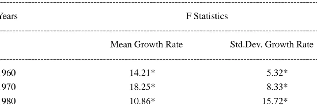
Table 1. The Goldfeld-Quandt Test

---

Years F Statistics

--- Mean Growth Rate Std.Dev. Growth Rate --- 1960 14.21* 5.32* 1970 18.25* 8.33* 1980 10.86* 15.72* --- Note: ₂ 1 2 2 S S F = .

(15)

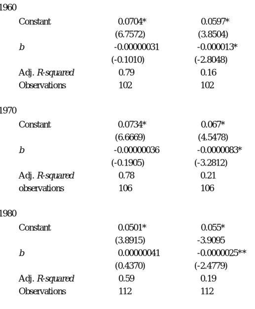
Table 2. Regression of the average and standard deviation of annual income growth rate on initial income

---

Average Growth Rate Standard.Deviation of Growth Rate

--- 1960 Constant 0.0704* 0.0597* (6.7572) (3.8504) b -0.00000031 -0.000013* (-0.1010) (-2.8048) Adj. R-squared 0.79 0.16 Observations 102 102 1970 Constant 0.0734* 0.067* (6.6669) (4.5478) b -0.00000036 -0.0000083* (-0.1905) (-3.2812) Adj. R-squared 0.78 0.21 observations 106 106 1980 Constant 0.0501* 0.055* (3.8915) -3.9095 b 0.00000041 -0.0000025** (0.4370) (-2.4779) Adj. R-squared 0.59 0.19 Observations 112 112 ---

Note:y =a+bx, where y is the average or the standard deviation of annual income growth rate, x is the initial income. Numbers in parentheses are t values.

The regression of generalized least squares is based on the result from Park test. *Significant at the 1% level.

(16)

Table 3. Regression of the average and standard deviation of income growth rate on initial income of group 1

---

--- 1960 Constant 0.0829 -0.0951 (0.6839) (-0.3225) b -0.0000051 0.000014 (-0.2888) (0.3344) Adj. R-squared 0.44 0.00 Observations 17 17 1970 Constant 0.049 -0.0386 (0.2314) (-0.0885) b -0.00000008 0.0000037 (-0.0494) (0.1085) Adj. R-squared 0.16 0.00 Observations 17 17 1980 Constant 0.2005 0.6863 (0.3075) (0.996) b -0.0000055 -0.000025 (-0.2624) (-0.9261) Adj. R-squared 0.00 0.04 Observations 17 17 ---

(17)

Table 4. Regression of the average and standard deviation of income growth rate on initial income of group 2

---

--- 1960 Constant 0.0419 0.0813** (1.7874) (2.4487) b 0.000016 -0.000023 (1.1794) (-1.1719) Adj. R-squared 0.52 0.18 Observations 85 85 1970 Constant 0.0518** 0.0823* (2.4261) (2.9900) b 0.0000065 -0.000012 (0.9836) (-1.4289) Adj. R-squared 0.55 0.23 Observations 89 89 1980 Constant 0.0517** 0.0084 (2.5598) (0.4082) b 0.00000001 0.0000044 (0.0044) (1.8997) Adj. R-squared 0.35 0.3 Observations 95 95 ---

*Significant at the 1% level. **Significant at the 5% level.

(18)

Table 5. Trend of Inequality

1960 ~ 1998

Index β (Group1) t β (Group2) t β (Total) t

β 0.0687* 5.4058 -0.0108* -21.9898 -0.0064* -25.7592 Gini -0.0012* -5.8728 0.0013* 4.0486 -0.0001 -0.2471 GE 0.0002 1.6513 -0.0026* -4.6102 -0.0014* -3.4939 GE' -0.0010* -8.1506 -0.0082* -3.2219 -0.0121* -4.8926 J 0.0031* 6.0908 -0.0074* -5.0350 -0.0029* -2.7674 J' 0.0054* 3.0085 -0.0610* -5.1937 -0.0418* -4.4857 Cov -0.0018* -4.3658 0.0051* 13.3184 0.0014* 5.3215 1960 ~ 1976

Index β (Group1) t β (Group2) t (Total) t

β 0.1550* 7.3395 -0.0161* -12.6064 -0.0100* -19.0138 Gini -0.0033* -8.7961 0.0035** 2.2828 0.0006 0.4431 GE 0.0022* 6.4437 0.0055* 12.8085 0.0040* 14.2382 GE' -0.0024* -4.7130 0.0244* 10.6795 0.0258* 12.3250 J 0.0015 1.2682 0.0130* 6.7688 0.0089* 12.4684 J' -0.0049 -1.2183 0.1056* 10.6834 0.0807* 12.5282 Cov -0.0062* -9.6316 0.0100* 13.6332 0.0017* 3.1491 1976 ~ 1998

Index β (Group1) t (Group2) t (Total) t

β -0.0527** -2.8031 -0.0071* -9.5216 -0.0048* -13.0036 Gini 0.0008* 3.7737 0.0013** 2.4347 0.0013* 3.2358 GE 0.0000 0.2740 -0.0078* -15.0143 -0.0052* -14.9110 GE' -0.0002 -1.5083 -0.0311* -9.6774 -0.0344* -17.4592 J 0.0025 1.7986 -0.0212* -16.9412 -0.0135* -13.3279 J' _0.0028 _{0.6098 -0.1721* -18.0875 -0.1357* -20.8877} Cov 0.0025* 5.4478 0.0031* 4.1292 0.0039* 10.8320

Note:y =a+bx, where y is inequality index; x is time trend. *Significant at the 1% level

(19)

Table 6. Time series analysis of measure of inequality

Index Group1 Group2 Total

β IMA(1,0) IMA(1,0) IMA(1,0)

Gini IMA(1,0) AR(1) White Noise

GE ARMA(1,1) IMA(1,0) IMA(1,0)

GE' IMA(1,0) IMA(1,0) IMA(1,0)

J AR(1) IMA(1,0) IMA(1,0)

J' AR(1) IMA(1,0) IMA(1,0)

(20)

Table 7 Descriptive Statistics and Pair t Test

--- A. Descriptive statistics

--- Variables Mean Std Dev. Min. Max. Pair t --- Total countries Oshima 5.516 2.967 10.725 20.657 Gini 0.499 0.020 0.472 0.555 GE 0.779 0.073 0.635 0.893 GE' 1.694 0.220 1.276 2.040 J 2.358 0.079 2.209 2.470 J' 10.987 0.804 9.389 12.093 Cov. 0.940 0.024 0.901 0.983 --- Group 1: higher income

β _5.547 _1.179 _3.647 _7.418 _23.65* Gini 0.082 0.019 0.059 0.120 -61.28* GE -0.039 0.021 -0.079 0.005 -40.39* GE' 0.034 0.015 0.016 0.070 -29.64* J 0.838 0.050 0.754 0.975 -69.39* J' 1.748 0.138 1.521 2.185 -51.35* Cov. 0.155 0.037 0.106 0.225 -47.93* --- Group 2: lower income

β _{1.071 0.128 0.903 1.328} Gini 0.407 0.027 0.350 0.471 GE 0.703 0.113 0.481 0.868 GE' 0.983 0.199 0.648 1.327 J 2.418 0.133 2.161 2.605 J' 10.625 1.071 8.598 12.122 Cov. 0.721 0.064 0.595 0.820 ---

Note: t is the test statistics for the Pair t Test.

n S d t d / = .

(21)

Table 8 Correlation Matrix

--- Total countries

---

Osh. Gini GE GE' J J' Cov.

Oshima 1.000 0.101 -0.354** -0.588* -0.245 -0.516* 0.696* Gini 0.101 1.000 -0.214 -0.210 -0.304 -0.276 0.446* GE -0.354** -0.214 1.000 0.936* 0.964* 0.960* -0.573* GE' -0.588* -0.210 0.936* 1.000 0.848* 0.976* -0.664* J -0.245 -0.304 0.964* 0.848* 1.000 0.907* -0.577* J' -0.516* -0.276 0.960* 0.976* 0.907* 1.000 -0.711* Cov. 0.696* 0.446* -0.573* -0.664* -0.577* -0.711* 1.000 --- Group 1 ---

β Gini GE GE' J J' Cov.

β 1.000 -0.965* 0.095 -0.803* 0.580* 0.347** -0.966* Gini -0.965* 1.000 -0.137 0.746* -0.520* -0.274 0.963* GE 0.095 -0.137 1.000 -0.266 0.009 -0.402** -0.186 GE' -0.803* 0.746* -0.266 1.000 -0.799* -0.505* 0.728* J 0.580* -0.520* 0.009 -0.799* 1.000 0.850* -0.489* J' 0.347** -0.274 -0.402 -0.505* 0.850* 1.000 -0.248 Cov -0.966* 0.963* -0.186 0.728* -0.489* -0.248 1.000 --- Group 2 --- β Gini GE GE' J J' Cov.

β 1.000 -0.537* 0.478* 0.434* 0.493* 0.527* -0.935* Gini -0.537* 1.000 -0.194 -0.147 -0.231 -0.238 0.545* GE 0.478* -0.194 1.000 0.976* 0.975* 0.990* -0.332** GE' 0.434* -0.147 0.976* 1.000 0.933* 0.963* -0.264 J 0.493* -0.231 0.975* 0.933* 1.000 0.985* -0.373** J' 0.527* -0.238 0.990* 0.963* 0.985* 1.000 -0.399** Cov -0.935* 0.545* -0.332** -0.264 -0.373** -0.399** 1.000 --- *Significant at the 1% level

(22)

Table 9. Inequality and growth (Tobit)

---

Inequality Index Constant b1 b2 R-square

---

Group I: Higher Income

β _3.27* _16.71* _0.0001* _0.40 (6.7161) (3.4302) (5.3645) Gini 0.12* -0.32* -0.0000019* 0.49 (16.8348) (-4.3955) (-6.2009) GE -0.029* 0.11** 0.00000035 0.09 (-5.7790) (2.3239) (1.7159) GE' 0.07* -0.21* -0.0000017* 0.64 (14.2108) (-4.5537) (-8.7066) J 0.78* 0.07 0.0000048* 0.44 (38.4698) -0.3212 -5.5842 J' 1.67* -0.17 0.0000081* 0.14 (23.8269) (-0.2462) -2.7753 Cov 0.23* -0.63* -0.0000030* 0.36 (14.6977) (-4.0425) (-4.6353)

Group 2:Lower Income

β _1.23* _0.03 _-0.000068* _0.84 (88.4452) (0.0722) (-14.1124) Gini 0.39* 0.43** 0.0000092* 0.26 (60.6676) (2.1119) (4.1485) GE 0.36* 0.05 -0.000022* 0.5 (36.2906) (0.1714) (-6.3597) GE' 0.07* -0.99 -0.000077* 0.32 (24.9483) (-0.6609) (-4.6861) J 2.57* 0.68 -0.0001* 0.56 (100.8802) (0.8400) (-6.8003) J' 11.88* 0.63 -0.0005* 0.56 (58.1665) (0.0968) (-7.1062) Cov 0.65* -0.09 0.000032* 0.71 (69.9070) (-0.3181) (9.7807) ---

Note: Numbers in parentheses are t values.

*Significant at the 1% level **Significant at the 5% level.

(23)

---

Inequality Index Constant b1 b2 R-square

--- Total Oshima 11.24* 25.86* 0.0012* 0.96 (68.9056) (2.8624) (31.1939) Gini 0.50* 0.23 0.00000011 -0.07 (81.7313) (0.6652) (0.0810) GE 0.37* 0.11 -0.0000083* 0.40 (51.7192) (0.2740) (-5.0832) GE' 1.96* 0.64 -0.000068* 0.58 (46.8568) (0.2782) (-7.1382) J 2.43* 0.61 -0.000018* 0.29 (123.817) (0.5584) (-3.9137) J' 11.89* 2.22 -0.0002* 0.51 (72.0462) (0.2429) (-6.2475) Cov 0.91* 0.59** 0.0000074* 0.48 (183.4586) (2.1410) (6.4796) ---

Note:y =a+b₁x₁+b₂x₂, where y is inequality index;x is the growth of mean ₁

income and x is the mean income. Numbers in parentheses are t values. 2 *Significant at the 1% level

(24)

(25)

0 2 4 6 8 10 12 14 16 18 100 600 1,100 1,600 2,100 2,600 3,100 GDP per capita 1960 (US$)

Percentage 0 2 4 6 8 10 12 14 16 18 0 1,000 2,000 3,000 4,000 5,000 GDP per capita 1970 (US$)

Percentage 0 2 4 6 8 10 12 14 16 18 0 2,500 5,000 7,500 10,000 12,500 GDP per capita 1980 (US$)

Percentage 0 2 4 6 8 10 12 14 0 7,200 14,400 21,600 28,800 36,000 GDP per capita 1998 (US$)

Percentage

(26)

0 1 2 3 4 5 0 1 2 3 4 5 6 7 8 9 Log(income) 1960 Log(rank) 0 1 2 3 4 5 0 1 2 3 4 5 6 7 8 9 Log(income) 1970 Log(rank) 0 1 2 3 4 5 0 1 2 3 4 5 6 7 8 9 10 Log(income) 1980 Log(rank) 0 1 2 3 4 5 6 0 1 2 3 4 5 6 7 8 9 10 11 Log(income) 1998 Log(rank)

(27)

0 0.02 0.04 0.06 0.08 0.1 0.12 0.14 0 500 1000 1500 2000 2500 3000 3500 Income 1960 (US$)

Average income growth rate

0 0.02 0.04 0.06 0.08 0.1 0.12 0.14 0 500 1000 1500 2000 2500 3000 3500 4000 4500 5000 5500 6000 Income 1970 (US$)

-0.02 0 0.02 0.04 0.06 0.08 0.1 0.12 0.14 0 1500 3000 4500 6000 7500 9000 10500 12000 13500 Income 1980 (US$)

-0.15 -0.1 -0.05 0 0.05 0.1 0.15 0.2 0.25 0 4000 8000 12000 16000 20000 24000 28000 32000 36000 40000 Income 1996 (US$)

(28)

0 0.03 0.06 0.09 0.12 0.15 0.18 0.21 0 500 1000 1500 2000 2500 3000 3500 Income 1960 (US$)

Standard deviation of income

growth rate 0 0.03 0.06 0.09 0.12 0.15 0.18 0.21 0.24 0 500 1000 1500 2000 2500 3000 3500 4000 4500 5000 5500 6000 Income 1970 (US$)

growth rate 0 0.04 0.08 0.12 0.16 0.2 0.24 0.28 0 1500 3000 4500 6000 7500 9000 10500 12000 13500 Income 1980 (US$)

growth rate 0 0.04 0.08 0.12 0.16 0.2 0.24 0 4000 8000 12000 16000 20000 24000 28000 32000 36000 40000 Income 1996 (US$)

growth rate

Figure 5. The standard deviation of income growth rate versus the initial income in 1960, 1980 and 1996.

(29)

Pareto coefficient 0 1.5 3 4.5 6 7.5 9 1960 1965 1970 1975 1980 1985 1990 1995 Year Group 1 Group 2 Total Gini 0 0.1 0.2 0.3 0.4 0.5 0.6 1960 1965 1970 1975 1980 1985 1990 1995 Year Group 1 Group 2 Total GE -0.1 0 0.1 0.2 0.3 0.4 0.5 1960 1965 1970 1975 1980 1985 1990 1995 Year Group 1 Group 2 Total GE ' -0.2 0.3 0.8 1.3 1.8 2.3 1960 1965 1970 1975 1980 1985 1990 1995 _Year Group 1 Group 2 Total

(30)

J 0 0.5 1 1.5 2 2.5 3 1960 1965 1970 1975 1980 1985 1990 1995 _Year Group 1 Group 2 Total J ' 0 2 4 6 8 10 12 14 1960 1965 1970 1975 1980 1985 1990 1995 Year Group 1 Group 2 Total Coefficient of Covariance 0 0.2 0.4 0.6 0.8 1 1.2 1960 1965 1970 1975 1980 1985 1990 1995 _Year Group 1 Group 2 Total

(31)

Mean income 0 5000 10000 15000 20000 25000 30000 1960 1965 1970 1975 1980 1985 1990 1995 Year Mean income Group 1 Group 2 Total

Mean income growth rate

-0.1 -0.05 0 0.05 0.1 0.15 0.2 1961 1966 1971 1976 1981 1986 1991 1996 Year

Mean income growth rate

Group 1 Group 2 Total

(32)

Population density 0 0.01 0.02 0.03 0.04 0.05 0.06 1960 1965 1970 1975 1980 1985 1990 1995 Year Population dens ity Group 1 Group 2 Total

Population density growth rate

-0.2 -0.15 -0.1 -0.05 0 0.05 0.1 0.15 0.2 0.25 1960 1965 1970 1975 1980 1985 1990 1995 Year

Population density growth

rate