Topological properties of incomplete WK-recursive networks

Topological Properties

of

Incomplete WK-Recursive Networks

Ming-Yang Su and Gen-Huey Chen Dyi-Rong Duh

Department of Computer Science and Information Engineering, Department of Elecuonic Engineering, Hwa Shia Junior College, Taipei, TAIWAN National Taiwan University, Taipei, TAIWAN

Abstract

The WK-recursive networks, which were originally proposed by Vecchia and Sanges, have suffered from the rigorous restriction on the number of nodes. Like the other incomplete network, the incomplete WK-recursive networks is proposed to relieve this restriction. In this paper, it is first shown that the structures of the incomplete WK-recursive networks are conveniently represented with multistage graphs. This representation can provide a unifbm look ut the incomplete WK-recursive networks. By its aid, we ( I ) compute the connectivities

of

the incomplete WK-recursive networks, ( 2 ) show that they are hamiltohian if their connectivities are greater than one, and ( 3 ) propa suficient and necessary condition for a hamiltonian path in an incompkte WK-recursive network with connectivity I .

1

Introduction

~ t, , : . i ,

In the recent decade, a number of networks ha$t.&en proposed in the literature 11. 5 , 15, 17, 18, 191. For these networks, many nice topological properties have been.derived and many efficient algorithms have been developed. However, a major defect of these networks

is

that they are not truly expansible. A network is expansible if no changes with respect to node configuration and link connections are necessary when it is expanded.

We have emphasized two topological advantages, i.e., expansibility and equal degree, with the consideration of easy implementation and low cost. Recently, the WK-recursive networks 1221 owning these two properties have been proposed. ll-icy offcr high degree of regularity, scalability and symmetry which very well conform to a modular design and implementation of distributed systems involving a large number of computing eleme.nts. A VLSI implementation of a

16-node WK-recursive network had been realized at the Hybrid Computing Research Center [22]. Later this prototype network had been further extended to 64 nodes [231. Some variants of the WK-recursive networks have been proposed recently [7,81.

Although the WK-recursive networks own many nice properties (see [4, 6, 9-11, 22, 231). there is a rigorous

restriction on the number of their nodes. As we will see in the next section, the number of nodes contained in a

WK-

recursive network is restricted to d , where d

is the degree and

t I S the level. Thus, as d = 4 ,

espa

3.47=49152 qgdas are

requiredqo expand from 7-level WK-recursive network to a &level WK-recursive network. Almost all of the networks mentioned earlier in this section suffered from the same problem. Therefore, some incomplete structures [12, 13, 14, 161 have been proposed as a soluhon to this problem.

In this paper, we define the incomplete WK-recursive networks that require

the

number of nodes

to

be a multiple of

d,

where d is the size of the basic building block. Since each basic building block of the WK-recursive networks contains d nodes, the incomplete WK-recursive networks can be expanded or contracted in arbitrary units of basic building blocks. We then compute the connectivities and hamiltonicity of the incomplete WK-recursive networks.

In the next section, the WK-recursive networks are reviewed and the incomplete WK-recursive networks are formally defined. The connectivities and hamiltonicity are discussed, respectivity, in Sections 3 and 4. Finally, this paper IS concluded with some remarks in Secuon 5.

2

WK-Recursive Networks

and

Incomplete

WK=Recursive Networks

The WK-recursive networks can be constructed recursively by grouping basic building blocks. Any complete graph can serve

as a

hasic building block. For convenience, we use K(d, t ) to denote a WK-recursive network of level

r

whose basic building blocks are each a d-node complete graph, where d>l and f > l . K(d, 1). which is the basic

building block, is a d-node complete graph, and K(d, t ) for t22 is composed of d K(d, t-1)’s which are connected as a complete graph. Each node of K(d, t ) has degree d and can be uniquely identified by a sequence of I digits. We define K(d, t ) formally

as

follows.

Definition 2.1. The node set of K(d, t ) is denoted by (al-lar+..alaO I a , € ( 0 , 1,

...,

d - 1 ) for O G s t - l } . Node adjacency is defined as follows: ar-lar-2

...

ala0 is adjacent to (1) a,-lat.2...nlb, where OSbld-1 and b;ea0, and (2) uz.lul-2

. . . u ; + ~ a ~ . l ( u ~ ) ~ ifa;;tai.l and aL.1=a;.2= ... = u l = u ~ , where ( u t ) ; represents i consecutive ud's. The links of ( 1) are named substiruling links and assigned label 0. The links of (2) are named ]Zipping links and assigned label i. The flipping links wiih label i are referred to as i-flipping links. Besides, there arc

open

links whose one end node is at, where Wu5.d-I, and

h e other end node is unspecified. The open links are labeled t .

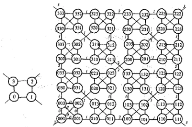
Since each node is incident with d-1 substituting links and one flipping link (or open link), K(d, t ) has degree d. The structures of K(4, 1) and K(4, 3) are illustrated in Figure 1. Intuitively, the substituting links are those within basic huilding blocks, the i-flipping links each connect two embedded K(d, i ) ' s , and the open links are left for future expansion. For example, let us consider the incident links of node 31 1 in Figure I . The one to node 133 is a 2-flipping link, and the others are substituting links.

Figure 1. The structures of K(4, 1) and ~ ( 4 , 3 ) .

Definition 2.2. Define ct-1ct-2

...

c,.K(d, r ) to be the induced subgraph of K(d, t ) by (cl.lcf.2 ... cp,l ... ala0 I ai E

(0, 1,

...,

d-1) for O%iSr-l}, ,where 1 9 3 - 1 and ct.l, Cr.2,

....

c r are all integers from {O, 1,

...,

d - 1 ) .

In Figure 1 , for example, 2O.K(4, 1) is the subgraph induced by (200, 201,202, 203).

Definition 2.3. Node u l . ~ a f - 2

...

ulao

is a k-frontier,

where Ilkst, if u k . 1 ~

...

=ul=ug.

Note that by Definition 2.3 a k-frontier is automatically an l-frontier, where 1 4 < k . Both end nodes of a k-flipping link

are k-frontiers. An embedded K(d, r ) contains one (r+l)- frontier and d-1 r-ffontiers.

Now, we begin to introduce the incomplete WK-recursive networks. The incomplete WK-recursive networks are subgraphs of the WK-recursive networks. For convenience, we use IK(d, t ) to denote an incomplete WK-recursive network with N nodes, where d f - ' d < d t is a multiple of d. The: restriction to N is because K ( d , 1 ) remains the basic

huilding block tor IK(d, t ) . The structure of IK(d, 2 ) with N nodes can he uniquely determined by the associated coefficient vector, as defined below

Definition 2.4. The coefjicient vector associated with an N-node I K ( d , I ) is a (t-l)-tuple (br-1, bt-2, ..., b l ) satisfying N=b,.idf-'+6t-2df-*+ ... +bid, where l<_b,.l<d- I and OGiSd- I for I <&I-2.

Let V(b,.l, b1.2.

...,

b l ) denote the node set of IK(d, f )

with coefficient vector (b(-l, 61-2,

....

61) and V(i.K(d, 2-11)

denote the node set of i . K ( d , f-l), where OGG-1. The set V(bf.l, br.2, ..., b l ) can be defined recursively as follows.

V(bt.1, br-2, ..., bl) = V(0-K(d, t- 1 ))+V( 1 .K(d, t - 1))+ ...

+V((bl-l- 1 ).K(d, t- 1 ))+V(br-i.(bt.z, br-3.

...,

b l ) ) ,

where

+

denotes a union operation and br-1.(bt-2, bt-3, ..., b ~ ) represents an Irf(d, t-1) with Coefficient vector (bf.2, br-3,

...,

bl) that is contained in bf-l.K(d, t-1) provided b,2#0. If br-2= bl.3

=

...

=b+O and b,-l?tO, where l<rSt-2, then bt-1.(bb.2,

b,-3,

...,

b l ) represents an IK(d, r ) with coefficient vector (

For example, the coefficient vector o f IK(5, 6) with 8225 nodes is (2, 3, 0, 4, 0) and its node set can be expressed as follows.

b,.2,

...,

61) that is contained in b,.lOt+'.K(d, r ) .

V(2, 3, 0, 4, 0 ) = V(O.K(5, 5))+V(l.K(5, 5))+V(2.(3, 0, 4, 0)) = V(O.K(5, 5))+V(l.K(5, 5))+V(20.K(5, 4))+V(21.K(5, 4)) +V(22.K(5, 4))+V(23.(0, 4, 0)) = V(O.K(5, 5))+V( l.K(5, 5))+V(20.K(5, 4))+V(21.K(5, 4))+V(22.K(5, 4))+V(230.(4, 0)) = V(O.K(5, 5))+V( 1 K(5, 5))+V(20.K(5, 4))+V(21.K(5, 4))+V(22.K(5,4))+V(2300.K(5, 2))+V(2301.K(5, 2))+V(2302.K(5, 2))+V(2303.K(5, 2))

The structure of IK(d, 2) with coefficient vector (b,.l, bt.2,

...,

61)

is

defined as follows.

Definition 2.5. IK(d, t ) with coefficient vector (bl.l,

b,.~,

...,

61) is the induced subgraph o f K(d, t ) by V(b,.], 61-2,

...,

b l ) .

See Figure 2 where the structure of IK(4, 3) with coefficient vector (3,2) is shown.

3

Connectivity

The connectivity of a connected network is defined as the minimum number of nodes whose removal can result in the network disconnected. Connectivity IS usually adopted as a

measure for fault tolerance in networks because Menger's theorem [3] states that the number of node-disjoint paths between two nodes of a network is at least its connectivity, Since 1K(d, I ) is a subgraph of K(d, t ) , the connectivity of the

former is not greater than the connectivity of the latter. The connectivity of K(d, t ) is known to he d-l 14). In this section, the connectivity of IK(d, t ) is computed. First, some necessary detinitions and lemmas are introduced.

I

Figure 2. The structures of IK(4.3) with

coefficient vector (3,2).

According to Definition 2.5, IK(d, t ) with coefficient vector (bl-l, br-2, ..., bl) contains b,.l embedded K(d, t-l)k, br-2 embedded K(d, t-2)'s.

...,

and bl embedded K(d, 1)'s. For 1SiSt-1, the b ; embedded K(d. i)'s are b,.lbr-z

...

b,+lO.K(d, i), bplbr-2..,.bi+i l . K ( d , i ) ,

...,

and br-1bt-2

...

b;+l(bi-l).K(d, i ) . Let G, represent the induced subgraph of IK(d, t ) with coefficient vector (bt.l, b,2, ..., b l ) by V(b,-l br-2

...

bi+l(bi-l ).K(d, i ) ) , and RY, where l<n<m<t-1, the

connectivity

o f

G,+G,-l+

...

+C,. Then, R;' is the connectivity of IK(d, t ) with coefficient vector (br-l, bt-2,

...,

bl). In Figure 2, for example, we have R:=2, R:=l, and the connectivity of theIK(4,3) is R:=2.

For easy reference, we refer to bt.lbr-z

...

b;+lr.K(d, i ) as the (r+l)th K(d, i ) within G, in the subsequent discussion, where OSrSbi-1. Besides, a coefficient vector ( b f - l , br-2,

...,

b l ) is written as @*.I, bl.2.

...,

bi, *), provided bl=b2=

...

=bi-l=O and bi+O. For example, ( 2 , 3, 0, 4, 0) is written as (2, 3, 0 , 4 , *), and (2, 3 , 4 ) is written as (2, 3 , 4 , *).

br-2.. bi+l O*K(d, i))+ V(br.1 bt-2.

..

bi+ll .K(d, i))+ .

..

+V(bt. 1

Lemma 3.1. For IK(d, I ) with coefficient vector (br-l,

m

bf.2,

...,

bi, *), R,=b,-1 ifb,>2, where 1SiimV-1.

Proof. C , can be regarded as a &-node complete graph with each node being a K(d, m). The connectivity of K(d, m ) is known to be d-1. Since at least b,-1 ( 4 1 ) nodes have to be removed in order to disconnect a bm-node complete graph, the connectivity of C, is bm-l. Hence, q = b m - l . Q.E.D.

Lemma 3.2. For IK(d. I ) with coefficient vector (bt-l, br-2,

....

bi, *), R;-,=min(b,-l, b,) if bm-121 and b,&l, where 1 li<mSt- 1.

Proof: We first assume h,<b,,.l. For O<jSb,-l. there is an m-flipping link between bf.Ibr-z... b,+j.K(d, m ) and h,. ~b,.?

...

b,J.K(d, n-1). There are several possihilities (and their combinations) to disconnect G,n+Gm-,. To isolate one or more nodes from a K(d. m- 1) or a K(d,

m )

requires removing at least d-1 nodes. To isolate one or more K(d.

m)'s

from G, requires removing at least b, nodes. To isolate one or more K(d, m-l)'s from Gm-l requires removing at least

f ~ , , . ~ -

1 nodes. To separate Gm.1 from

G,

requires removing at least bm nodes. Hence, the connectivity of G,+Gm.l is b,.

With similar arguments, the connectivity of Gm+C,-l can be proved 'to be b, if bm=bm-l, and b,.l if b,>b,.l. This

completes the proof. Q.E.D.

Lemma 3.3, For IK(d, I ) with coefficient vector ( & I , br-2, ..., bi, *), R m - t -b,+1 if bm+l>bm and b,<b,-l, and

min(bm+l,

b,, b,,.l)

else,

where bm+121, b,>O, bm.121, and 1 S i 4 n a - 2 .

Proof. There are five cases: ( 1 ) bm+lSbmSbm-l; ( 2 )

m + l -

bm+lZbmSbm-l; (3) bm+~<bm and bm>bm-l; (4) bm+l>bmr bm<bm-l, and b,+O: ( 5 ) b,=O, to be considered.

Case 1. bm+lSbmSbm-l.

Note that for i<j<r-l. there

are

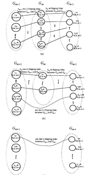
mintb), bj-1) j-flipping links corinecting C, and Gj-1. By Lemma 3.2, RZ+'=b,+l and Rt-,=bm. Since no link exists between Gm+l and G,.,

(see

Figure 3(a) where the links among each

Gj

are

omitted), the connectivity of Gm+l+Gm+Cm-I is bm+1.

Case 2. bm+12b,2bm.1.

and R m-l=bm-l. The connectivity of Gm+l+Gm+Gm-l is b,.1 with the arguments similar to Case 1.

Case 3. bm+l<bm and bm>b,-l,

By Lemma 3.2, R"+'=b,,z and R",I=b,-l. The connectivity of Cm+l+Gm+Gm-l is mintb,+l, bm.1) with the arguments similar to Case 1.

Case 4. bm+l>bm, b,<b,-l, and b,&.

By Lemma 3.2, R:+'=bm and R:-,=b,. There.are b,

(m+l )-flipping links, i.e., (br-l&f-~... bm+20(bm+l)m+l, b,.l

m

By Lemma 3.2, R::,+'=b,

br.2 ...bm+zbm+lOm+l), (br-1 br-2.. .bm+2 l ( b m + ~ ) ~ + ' . br.1 br.2

...

bm+zbm+l lm+')v

...)

and (b,-lbt-z...bm+2(bm-l )(bm+l)m+l, br-1

br.2...bm+2b,+l(b,-I)m+1), between G,+l and G , (see

Figure 3(b)). Besides, there is exactly one (m+l)-flipping link between Gm+l and Gm-l as explained as follows. There is an

(m+

1 )-flipping link, i.e., (bt.1 bt.2.. .bm+zbm(bm+l P + l l br- 1

br-2...bm+zbm+l (bmIm+1), connecting br-lbt-2

...

bm+2b,.K(d,

m + l ) and br.lbr-2

...

b,+2b,+lb,b,.K(d, m-1) which belong to C m + l and Cm-l, respectively. For j>bm, the link (br-lbr-2

because br.lbt.2

...

bm+2bnt+ljm+l is nnt a node i n the IK(d, t ) . Hencc. the connectivity O~G',+~+G~+G,.I is b,+l.

Case S.

o,,=o.

3(c)). The connectivity of G',,+I+G,+G,.J is 1 .

This case I S a degenerated case o f Case 4 (see Figure Q.E.D.

.. . , , , i

Figure 3. The pmofof Lemma 3.3. (a) Case 1 . (b) Case 4. (c) Case 5.

Lemma 3.4. For IK(d, t ) with coefficieni vector (b,.~. ..., b,,, r , ..., r . b,, ..., b , , * I (i.e., b,.l =bm.2= ...

=bn+l=r), where l l i i n < m i r - 1. m>n+2. b,>r, b,,>r. and OIr5d-2, R:=r+I. Moreover. there exists exactly one rn- flipping link between

G m

and G,, and n o other link exists between G, and Gv, where m<nSl-1 and

i<v<n.

proof BY Lemma 3.2,

q-l=~z::=

...

=R,, -r. It is not difficult to see that for n+lSckSm-2 and n+25IIm-l, no link exists between G, and C k and between Gn and GI. With the

arguments similar to Case 4 in the proof of Lemma 3.3, there

is exactly one m-flipping link, i.e., (br-lbt-2 ... bm+lr (b m I m , b,-1b?-2...b,+~b,r,), between G, and G,. Hence, the connectivity of Gm+Gm.l+

...

+G, is r + l .

Then we proceed to show that nd other link exists between G, and G,. W e first assume n t m and y;en, If a (x- flipping) link exists between G, and G,, its two end nodes should be br-lbt.z

...

bX+la(b,)* andb,lb,.z

...

b

some a i r . However, since x > m and a>r, bt.lbt-2

...

b,+lb,(aF is not a node in the IK(d, t). Similar1

proved that no link exists between G, and Cy

i S y a or m a - 1 and y=n.

n + l -

Q.E.D. Theorem 3.1. For IK(d, t ) with coefficient vector b,.z,

...,

bj, *), lIi<f-1, its connectivity, i.e., R;-' can be determined as follows.

(1) Ifi=t-l, then ~ ; ' = b , l - l .

(2) Otherwise, letting k=min{bf.l, b1..2,

...,

b i ) , R f ' = k i f b,.l=k or bi=k, and k+l else.

Proof. We prove this theorem by induction on i.

Induction basis. Lemmas 3.1, 3.2, and 3.3 show the validity of the theorem for i=t-1, t-2, and t-3, respectively.

Induction hypothesis. Assume the theorem is valid for i=m+l, where 11mIt-4. Let k'=min ( bl-l, bt.2, .._, bm+l ). Induction step. W e now discuss the.case of i=m. Three cases

are considered according to the value ofk'. Case 1. k'=bf-l.

In this case RL:l=bt.l. Since bl.1Sbf-2,

no

link emits from

GI-1 to G,, where mSjSt-3. Consequently, removing b,.I nodes will seperate Gt-t from G14+Gt-3+

...

+G,. W e first assume bm+l<bm. By Lemma 3.2 we have C'=b,+l. There are three possibilities (or their combinations) to disconnect

Gt-t+G1-2+ ... +Gm. One is io disconnect G, which requires removing at least bm+l nodes. Another is to seperate G, from

Gt.l+Gt-2+ ... +G,+l which requires removing at least bm+,

nodes. The other is to disconnect GI.1+G1.2+

...

+ G m + l which requires removing at least bt.1 nodes. Hence,

R , =min{b,.t, b , + ~ f = b ~ - l . Note that bt-l=min(bt.l, bf.2, ...,

On the other hand, i f b,+lsb,, $+l=bm by Lemma 3.2,

and no link emits from G , to GI, where m+2<l<t- 1 .

1- 1

Similarly, R:' can he determined as min(br.l, b,). Note that sincc bI.I=min(br.,, b1-2, ..., b m + l ) , min{b,.I, b,)=min(

!),-I, h 1 . z . ..., & + I . bm)

.

C a e 2. k'=b,+l.

hi this case R k y l = b m + l . If br-i=br-2=

...

=&,+I, the discussion is the same as Case 1 because b,.l =k'. Otherwise, let j = m i n ( I I m+Z<l<f-l and bpb,+l ). If bm+i<bm, by Lemma 3.4 there is aj-flipping link between G, and Gj. Also note that no link exists between G, and G, for s#j and

s#m+l. If b,+lzb,, no link exists between G, and G, for

s # m + l . With the arguments similar to Case 1. it can be

proved that $l=bm+l+1 and b,+l=minIbt-l, bt-2,

....

bm+L7 b,) if bm+l<bm, and Rk'=b, and b,=min(b,.l, br-2,

...,

b,+l.

&,I

else.

Case 3. k'#bf.1 and k'itb,+i.

We assume k'=b,, where m + l < r < f - l . In this case R;:,=b,+l. Letj=max{ E I m < k r and bpb,]. By Lemma 3.4, no link exists between G, and Gi, wherej<slf-1. With the arguments similar to Case 1, it can be proved that (1) if bm+lSb,, Rt'=b,+l and b,=min(bf-l, bl-2,

...,

b,,

...,

b,+l, b,); (2) if bm+l>bm and b&r+l, R, =bm and b,=min(bt-l, bf.z,

...,

b,,

...,

bm+l, b,

1

; (3) if bm+l> b, and b,>b,+l, R"'=b,+I m and bimin{b,.l, bf-2,

...,

b,,

...,

b,+l, b,).

Q.E.D. 1-1

We have the following corollary immediately.

Corollary 3.1. For IK(d, t) with coefficient vector (

br-1, bf-2,

...,

bi, *), letting k=min( b,, bm-l,

...,

b n ) , where

lSi9wn51-1, b,&, and b,&, R,"=k if b,=k or b,=k, and k+l else.

For iSncmY-1, an m-flipping link between G, and G, is called a jumping m-flipping link if m-n>l. Note that by

Lemma 3.4 the flipping links of an IK(d, t ) witEl coefficient

vector (bf-l, bI-2,

...,

bi, *) can be determined from its coefficient vector. We take IK(6, IO) with coefficient vector

(4, 3, 4, 2, 1, 1, 3, *) as an illustrative example. There are two jumping flipping links. One is between the 4th K(6, 9) within Gc, and the 4th K(6, 7) within G7, and the other is

between the 2nd K(6, 6) within Gg and the 2nd K(6, 3) within G3. An easy way to determine jumping flipping links is that for any local minimal value, say b,, in the sequence bf.l, bf-2, ..., bi, there exists a jumping (m-flipping) link between G, and G,, where i<r<t-1 and m=min ( I I r<llt- 1

and bpb,) and n=max(l I i S k r and bpb,), i f m and n exist. This link connects the (b,+l)th K(d, m ) and the (b,+l)th K(d,

n ) . All non-jumping flipping links exist between G , and Gm-l, where icm5r-1. More specifically, min(b,, bm-l) m- flipping links connect thejth K(d, m ) within G, and thejth K(d, m-1) within G,.1 for all l<Fmin(bm, bm-1).

4

Hamiltonicity

A cycle (path) in a network IS called a hamiltonran cvcle (path) i f i t contans every node of the network exactly once A

network is hamrlfonian i f it contains a hamltonian cycle A hamiltonian network can embed a ring with unit expansion and unit dilation. In this section, we show that IK(d, I) with connectivity greater than one is hamiltonian. Moreover, we propose a sufficient and necessary condition for a hamltonian path in an IK(d, I ) with connectivity one. Chen and Duh [41 have shown that K(2, t ) contains a hamiltonian path, and K(d, t) contains a hamltonian cycle for &3. Moreover, they have shown the following result.

Lemma 4.1. [4] There is one hamiltonian path between any two r-frontiers in K(d, f).

Since IK(2, t ) has a linear structure, it contains

a

hamiltonian path. In this section, we concentrate our attention on the hamiltonicity of IK(Q I) for d>3. First we adapt Lemma 4.1 to

IK(d,

I).

Lemma 4.2. There are two hamiltonian paths, one between 0' and 1' and the other between O(b,-l)f-l and l(l~[-l)~-l, in IK(d, 1 ) with coefficient vector *), where bt.122.

Proof: A hamiltonian path between 0' and 1' can be constructed as follows:

0' -+(H,1-1) O(bt-l-l)f-l

-+

(bf-I-l)Of-' j ( H . f - 1 ) (b,-i-l)(bf-1-2)~-' -+ (bf.1-2)(bt-i-l)f-1 +[H,f-l) (br-1-2) (bf-i-3)'-' 3 (b,-1-3)(b1-1-2)'-' -+(M,f-l) "' + ( H , f - i )

21'-' 12l-l +(H+J-~) It,

where

-+

indicates a flipping link and + ( ~ . ~ - l ) indicates a hamiltonian path i n a K(d, f-1). A hamltonian path between O(bf-l)f-i and l(bf-l)f-i can be obtained by substituting O( bf.l)f-l and l ( b , - ~ ) ~ - l , respectively, for 0' and 1' in the construction above. The correctness is assured by Lemma

4.1. Q.E.D.

Lemma 4.3. There are two node-disjoint paths, one between O(bf-l)f-l and 0' and the other between l(b[-~)'-~ and

If, in IK(d, f ) with coefficient vector (&I, *), where br.1>2,

such that they contam every node of the K ( d , 2 ) exactly once. Proof. There are b,-l K(d, t-lys, i.e., O.K(d, f - I ) , l.K(d, f - l ) , 2.K(d, f-l),

...,

and (br-l-l) K(d, f - l ) , contained

In the

IK(d, I ) . Clearly, O(bf-l)f-l, Of, l(bt-l)f-l, and 1' are all (1-1)-

frontiers, We consmct two node-disjoint paths according to the following two cases.

By Lemma 4.1, there is one hamiltonian path between O ( h r - , ) r - l and 0' in O.K(d, 2 - 1 ) . Likewise, there is one hamiltonian path hetween l(hl.l)f-l and 1' in l.K(d, 1-1). These two paths are node-disjoint, and they contain every node of the IK(d, 2 ) exactly once.

Case 2. b,1>2.

Note that O.K(d, t - 1 ) is composed of OO,K(d, t-2), Ol.K(d, t-2), 02.K(d, t-2), ..., and O(d-1). K(d, t-2), and

I,K ( d, t - 1 ) is composed of lO.K(d, t-2), lI.K(d, t-2), 12.K(d, t-2),

...,

and l(d-l),K(d, t-2). A path between O( br.1 )r-i and 0' is constructed as follows:

-+(HJ.~) 0&f.l(bf.1+1)'-2 -+ O(b&l+1)(b&1)'-2

- + [ H , f - 2 ) 0(b,l+1)(bt.1+2)'-2

-+

0(bf.1+2)(bt.1+1)'-2

+(HJ-~) ". +[H&2) o(d-1)@-2 -+ 00(d-1)f-2 -+(H,f-2)

o',

where

-+

indicates a flipping link and +(H,tJ) indicates a hamiltonian path in a K(d, f-2). The hamiltonicity is assured by Lemma 4.1. Actually this path contains every node of 0

O(d-l).K(d, t-2),'and OO.K(d, t-2) exactly once.

consmcted as the concatenation of the following

four

paths: b,.l.K(d, t-2), O(bt.l+l).K(d, t-2), O(b,1+2).K(d, t-2), ,..,

On the other hand, a path between l(bt-l)r-l and l C is

(1) 'l(bi.l)f-i ~ ( H J - 2 ) lbf-l(br-1+1)f-2 3 1(bt.l+1)(bt.l)f-2 +(H,f.2) 1(bf-1+1)(b&1+2)'-2

-+

1(b,-]+2)(b&1+1 j ( H . f - 2 ) ' " "(H.1-2) l(d-1)0f-2

-+

10(d-1)f-2 "[H,r.2) I @ * 0Ir-'; ( 2 ) 01'-l + - ( H , t - 2 ) 012L-2

+

021r-2 - + ( H , f - 2 ) 023f-2

-+

032'-2 + ( H , t - 2 ) "" j ( H , 1 . 2 ) O(bt-1-2)(br-l-l ) r - 2

*

O(bt.l-1)(bt-1-2)f'2 *(H,&2) O(6f-1-l)f-1 -$ (bf-1- 1 )Of-';

(3) (bt-1-1

)or-'

j ( H . t . 1 ) (b(.1-1)(bt-1-2)'-' -+ (b(-1-2)(bt-1- I)'-' +(H,i-l) (b~i-2)(bf-i-3)~-' -+(H,f-l) ..' *(H,f-l) 32'-'

+

23'-' -+(H,t-l) 21'-'+ 12"';

(4) 12'-' +(HJ-~) 1 2 3 ' ~ ~ 132I-2 + ( H , J - ~ ) 134f-2

143'-2 + ( H , f - 2 )

...

j ( H J - 2 ) 1(bf-1-2)(bf-1-1)t-2 4

l(bt.1-l)(br.1-2)'-~ +-(H,r.2) l(bt-l-l)l'-'

+

1 l(bt-1- l)r-2 +(H,f-2) 1'9

where ihe hamiltonicity is assured by Lemma 4.1. Path (1) contains all nodes of lbf-l.K(d, t-2). I ( bf-l+l).K(d, t-21, -., l(d-l)-K(d, t-2), and lO.K(d, t-2). Path (2) contains ail nodes of OI.K(d, t-21, 02K(d, f-21,

...,

and O(bz-l-I).K(d, t- 2). Path (3) contains all nodes of (br-l-l).K(d, f-l), (bf-l-2 ).K(d, t-l),

....

and 2,K(d, t - I ) . Path (4) contains all nodes

oJ

12.K(d, f-2). 13.K(d,t-2),

...,

l(bt.l-l).K(d, t-21, and 1 I.K(d, t-2). All nodes appear in these paths exactly once. It is not difficult to check that the two paths we have constructed

between O(bc-l)'-l and Of and between l(bc-l)f-i and 1' are

node-disjoint, and they contain every node of the IK(d, t )

exactly once. To illustrate the construction, Figure 4 shows two node-disjoint paths. one between 033 and 000 and the other between 133 and 1 1 1, i n IK(4, 3) with coefficient

vector (3. *). Q.E.D.

Figure 4. Two nodedisjoint paths, one between 033 and 000 and the other between 133 and 1 I 1 In IK(4.3) with coefficient vector (3.4

A necessary condition €or a hamiltinian graph is that its

connectivity must be greater than 1. In the following, we show that the latter is also a sufficient condition for a hamiltonian IK(d, t).

Theorem 4.1. An IK(d, t). where &3, 1s hamiltonian if its connectivity is greater than 1.

Proof. Suppose ( h - 1 , br-2,

...,

b,, *) is the coefficient

vector of the IK(d, f ) and R:-'>l. If i=t-1, by Theorem 3.1

we have bf.1>3. The IK(d, 1 ) is composed of bf_l K(d, t - 1 ) ' s

that are connected as a b,-l-node complete graph. By the ad

of Lemma 4.1, it is not difficult to see that there exists a hamiltonian cycle in the M(d, t). So, in the rest of the proof, we assume K i d - 1 . By Theorem 3.1 we have &t-122 and b,22. By Lemma 4.2, there exists a path between O(b,.,)~-J and l(bt-#-i which contains every node of Gf-l exactly once, and there exists a path between bf-~bt-2...br+10~+i and 6t-l b, 2... br+l lr+l which contains every node of G, exactly once. Since R:-'>l, we have b,>l for all i<m<Z-l. A hamltonian cycle in the IK(d, t ) is constructed according to the following two cases.

Case 1. b&2 for all ianet- 1.

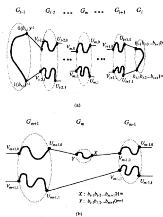
Lemma 4.3 assures that for k m c t - I , there exist two node-disjoint paths i n G,, one between Um,~=br-1bt.2

b,+lO(b,)m and Vm,0=b1-~br-2

...

bm+iOmfl and the other between Um,l=br-lbr-2

...

bm+l l(b,), and Vm,l=bf-lbt-2 .

bm+1lm+l, such that they contain every node of G, exactly once. A hamiltonian cycle in the IK(d, t ) is thus formed as

( O ( ~ , . I ) ' - ~ , Vr-2.0) and ( l ( h t . i F I , VI.2,1) define two ( t - I ) - nipping links;

( U i + l . o . h , . l h t . ~ . . . b , + l c ) i + ~ ) and ( U i + l , l , br.~hr.? ...

/ ~ , + ~ l i + ~ ) dcfine two (i+l)-tlipping links;

(U,,.o. V,.l,o) and (U,,,, Vn7.1,1) define two m-flipping links. where i+lcm<t-l.

Case 2. bm=l for

one or

more m's between i and f - 1 .

We assume b,,=l for exactly

one

m . The extension to

multiple m's is very straightforward. According to Lemma 4.1, there exists

a

path between X=br.lbt-2

..

.bm+lOlm and Y=hr-lbr-2 ... bm+lOm+i which contains every node of G, exactly once. As shown in Figure 5(b), there is an (m+l)- flipping link between Um+l,O and Y , an m-flipping link between

X

and Vm-l,O, and a jumping (m+l)-flipping link between Um+l,l and V m - l , l . A hamiltonian cycle in the M(d,

t ) can be constructed similar to Case 1.

Q.E.D.

,... .. .,

,- I

. . -,.,-,.C..bm+lOm+l

(b)

Figure 5. The proof of Theorem 4.1. (a) Case. 1. (b) Case 2

Theorem 4.1 guarantees a hamiltonian cycle in IK(d, t ) with d23 if its connectivity is greater than 1. For IK(d, t) with

connectivity 1, there is no hamiltonian cycle, and there is not necessarily a hamiltonian path. For example, no hamiltonian path exists in IK(4,4) with coefficient vector (1, 2, 1, *). In

what foliows, we identify the class of lK(d, f)'s with

connectivity 1 which contain a hamiltonian path.

For IK(d, t! with coefficient vector (h,.,, h,.?, ..,, h;. * I and R;'=l, we can partition it into hlocks. C;k is a b/oc.k 1 1

bk#O and ( R Y ' = l

or

b k + l = O ) and ( R i * , = l or l ~ k . ~ = O ) .

G m + G m - i + ... +G,, where b , d , b n d and m x , is a block ifR:>I and (R:+'=1 or bm+1=0) and (R:+l=l

or

b,+1=0). The partition can be easily done by examining the coefficient vector. As an illustrative example let us consider IK(6, 10) with coefficient vector (1, 2, 1, 2, 0, 1, *). By Lemma 3.4, there are two jumping flipping links. One is between the 2nd K(6, 8) within G8 and the 2nd K(6, 6) within G6, and the other is between the first K(6, 6) within G6 and the first K(6, 4) within G4. Clearly G9 and G4 are two blocks because

R ~ = I and b5=0, respectively. ~ 8 + ~ 7 + ~ 6 is another block because R:=2, R:=l, and b5=O. Hence IK(6, 10) with coefficient vector (1. 2, 1, 2, 0 , 1 , *) can be partitioned into

{G9,

Gs+G7+G6, G4}. Intuitively, if each G, (4SjS9) with b,& is regarded as a node, then the flipping links between G9

and Gs and between G6 and G4 are two bridge6 I21, and each block is either a single node or a maximal biconnected component in the resulting graph. The following two lemmas have proven in [20].

Lemma 4.4.[20] An IK(d, t ) with connectivity 1 contains

a

hamiltonian path if it consists of one

or

two blocks.

Lemma 4.5.[20] Consider

an

IK(d, t) with coefficient vector (&,-I, b,-2,

...,

bi, *) and Ri-'=l that contains three or more blocks. There is a hamiltonian path in the IK(d, t ) if and only if for each block, say Gm+Gm-l+

...

+G,, in the IK(d,

t ) , no b,+l, b,, b,.l, ..., b,, bS.1 exist such that br+l E { O , l ) , bi.br.l=

...

=b,=2, b,.l E { O , I ) , and r-s+l is odd, where

m H - I , n#i, and nSsSrS m.

Combining Lemmas 4.4 and 4.5, we have

a

necessary and sufficient condition for a hamiltonian path in

an

IK(d, t ) with connectivity 1.

Theorem 4.2. For IK(d, t) with coefficient vector (bl.i, bl.z, ..., b,, *) and Rf'=l, it contains a hamiltonian path if and only if either of the following two conditions holds: ( I ) it contains one or two blocks;

(2) for each block, say Gm+Gm.l+

...

+G,, in the IK(d, t),

no b,l, &,, b r - l ,

...,

b,, b,.l exist such that &,+I E (0,

I}, b,=br-l=

...

=b,=2, b , . l E (0, l}, and r-s+l is odd, where m#t-1, n#i, and n S S r S m.

5

Concluding Remarks

Deriving topological properties for incomplete networks is

that complete networks of different sizes preserve great

topological similarity, whereas incomplete networks may have a significant difference i n their topologies. For example, K(d,

I ) looks very similar to K(d, r-I), whereas two I K ( d 0's with different coefficieiit vectors may look very unlike i n their topologies. Many of topological properties of the incomplete

star networks [13], 1161 are still unknown, although they have been well solved for the star networks [l]. Most of the results obtained for the incomplete

star

networks are restricted to a special case: N=c&!, where N is the number of nodes.

In this paper, we have shown i t very convenient to

represent the structure of an incomplete WK-recursive networks by a "multistage-like" graph G,-l+Gt.2+

...

+G;.

This representation provides a uniform look at the incomplete WK-recursive networks, and thus facilitates the derivation of many properties. By the aid of this representation, we have computed the connectivities and hamiltonicity. Moreover, we have suggested a tight upper bound on the diameters. The methods adopted in this paper are different from Chen and Duh's for the WK-recursive networks [4]. Readers who are interested in the incomplete WK-recursive networks

are

refered to [20] and I211 for more results. Precisely, using the prune-and-search technique a linear-time algorithm for computing the diameters can be found i n [20], and a distributed shortest-path routing algorithm can be found in 1211.

References

S. B. Akers and B. Krishnamurthy, "A group-theoretic model for symmetry interconnection networks," IEEE Trans.

on

Computers, vol. 38, no. 4, pp. 555-566, 1989.

J. Bondy and U. Murthy, Graph Theory with Applications, Macmillan Press, 1976.

F. Buckley and F. Harary, Distance in Graph, Addison- Wesley, 1990.

G . H. Chen and D. R. Duh, "Topological properties, communication, and computation on WK-recursive networks," Networks, vol. 24, no. 6, pp. 303-317, 1994.

P. Corbett, "Rotator graphs: an efficient topology for point-to-point multiprocessor networks," IEEE Trans.

on

Parallel and Distributed Systems, vol. 3, no. 5, pp.

D. R. Duh and G . H. Chen, "Topological properties of

WK-recursive networks," J . of Parallel and Distributed Computing, vol. 23, pp. 468-474, 1994.

R. Fernandes, "Recursive interconnection networks for multicomputer networks," in Proc. of rhe Int. Conf.on Parallel Processing, vol. 1, pp. 76-79, 1992.

R. Fernandes and A. Kanevsky, "Hierarchical WK- recursive topologies for multicomputer systems," in Proc. of the Int. Conf.on Parallel Processing, vol. 1, 622-626, 1992.

pp. 315-318, 1993.

[Y] R . Fernandes and A. Kanevsky, "Substructure allocation in recursive interconnection networks," in Proi'. of the int. Conf.on Parallel Processing. vol. I . (101 R. Fernandes. D. K. Griesen, and A. Kanevsky. "Efficient routing and broadcasting in recursive interconnection networks," in Proc. ofthe Int. Conf.on Parallel Processing, 1994, pp. 51-58.

[ I l l R. Fernandes, D . K. Friesen, and A. Kanevsky, "Embedding rings in recursive networks," in Proc. of Int. Symp. on Parallel and Distributed Processing, Oct. 1121 H. P. Katseff, "Incomplete hypercubes," IEEE Trans.

on

Computers, vol. C-37, no. 5, pp. 604-608, 1988. [13] S . Latifi and N. Bagherzadeh, "Incomplete star: an

incrementally scalable network based on the s t k graph," IEEE Trans.

on

Parallel

and

Distributed Systems, vol. 5 , no. 1, pp. 97-102, 1994.

[14] S . Ponnuswamy and V. Chaudhary, "Embedding of

cycles in rotator and incomplete rotator graphs," in P r o c . of Int. Symp. on Pafallel and Distributed Processing, Oct. 1994, pp. 603-610.

[ 151 F. P. Preparata and J . Vuillemin, "The cube-connected cycles: a versatile network for parallel computation," Communications

of

the ACM, vol. 24, no. 5, pp. 300- 309, 1981.

[16] C. P. Ravikumar, A. Kuchlous, and G . Manimaran, "Incomplete star graph: an economical fault-tolerant interconnection network," in Proc. of h k . C o n f .

on

Parallel Processing, vol. 1, 1993, pp. 83-90,

[17] Y. Saad and M. H. Schultz, "Topological propekes of

hypercubes," IEEE Transactions

on

Computers, vol. 37, no. 7, pp. 867-872, 1988.

[18] M. R. Samatham and'D. K. Pradhan, T h e . d e Bruijn

multiprocessor networks: a versatile parallel' processing and sorting networks for VcSI,*' IEEE Trans. on Computers, vo!. 38, pp. 567-581, 1989.

[19] H. S. Stone, "Parallel processing with the perfect shuffle," IEEE Trans. on Computers, vol. 20, no. 2,

[20] M. Y. Su, G . H. Chen, and D. R. Duh, "Topological properties of incomplete WK-recursive networks," Tech. Rep. NTUCSIE 95-06, National, Taiwan University, Taipei, Taiwan, MarchJ995.

[21] M. Y . Su, G . H. Chen, and D. R. Duh, "A shortest- path routing algorithm for the incomplete WK-recursive networks," Tech. Rep. NTUCSIE 95-07, National Taiwan University, Taipei, Taiwan, July 1995. [22] G. D. Vccchia and C . Sangcs, "A recursively scalable

network VLSI implementation," Future Generation Computer Systems, vol. 4, no. 3, pp. 235-243, 1988. [23] G . D. Vecchia and C. Sanges, "An optimized

broadcasting technique for WK-recursive topologies," Future Generation Computer Systems, vol. 4, no. 3, 1993, pp. 319-322.

1994, pp. 273-280.

pp. 153-161, 1971.