用於高傳輸率渦輪碼之交錯器設計

全文

(1)國立交通大學電信工程學系博士論文用於高傳輸率渦輪碼之交錯器設計 Inter-Block Permutation Interleaver Design for High Throughput Turbo Codes 研究生：鄭延修指導教授：蘇育德. 中. 華. 民. 國九十六年十月.

(2) 用於高傳輸率渦輪碼之交錯器設計 Inter-Block Permutation Interleaver Design for High Throughput Turbo Codes 研究生：鄭延修. Student: Yan-Xiu Zheng. 指導教授：蘇育德. Advisor: Yu Ted Su. 國立交通大學電信工程學系博士論文 A Dissertation Submitted to Institute of Communication Engineering College of Electrical and Computer Engineering National Chiao Tung University in Partial Fulfillment of the Requirements for the Degree of Doctor of Philosophy in Communication Engineering Hsinchu, Taiwan 2007 年 10 月.

(3) 用於高傳輸率渦輪碼之交錯器設計研究生：鄭延修. 指導教授：蘇育德. 國立交通大學電信工程研究學系. 中文摘要渦輪碼以其優異的性能獲得通訊界的青睞，但為達到較佳的效能，渦輪碼需要進行較多次的遞回運算並搭配較長的交錯器，也因此造成較長的解碼延遲。因此我們提出一種系統化的交錯器設計流程去解決解碼延遲與解碼效能之間的兩難。我們的設計考量代數特性與硬體限制。從代數特性的觀點來看，此設計利用較短的交錯器去建構較長的交錯器以保持較佳的碼距特性，我們所提出的交錯器還可額外滿足高解碼率與平行解碼的硬體限制，其中包括避免記憶體衝突，有限的網路複雜度以及較簡單的記憶體控制線路。所提出的交錯器有較簡單的代數形式，也允許較有彈性的平行度並較容易適應各種不同的交錯器長度。就算並非應用於平行解碼，在相同的交錯器長度下，本設計亦提供較佳的碼距特性。我們將區塊間交錯重排交錯器分成方塊式與串接式，針對兩者我們為重量為二的輸入序列推導碼重邊界，此推導亦給了我們設計區塊間重排交錯器的參考依據，我們另外證明為了達成好的碼重性質並避免記憶體競爭的代數性質。針對方塊式區塊間重排交錯器，我們提出記憶體配置函數去描述與提供具彈性的解碼器平行度與支援高基數後驗機率解碼器。網路導向設計概念解決了平行解碼架構下網路複雜度的問題。我們亦提出有效率的交錯器設計流程去做大範圍的交錯器設. i.

(4) 計。我們亦用一個超大型積體電路設計去展現本設計確可同時兼顧高速與低複雜並提供較好的錯誤率。串接式區塊間交錯排列交錯器是針對導管型解碼架構而設計，此架構非常適合高解碼率應用但須付出複雜度的代價。為了得到複雜度與解碼率的最佳折衷點，我們提出了一個動態結構。我們處理其所面對的解碼排程與記憶體控制問題，我們亦介紹了一種新穎的結合冗餘檢測碼與正負號檢測的終止機制，在一個較佳的解碼排程，記憶體控管與終止機制下，我們可以減少硬體複雜度並在較短的平均解碼延遲下達成更好的錯誤率。為了描述各種遞回式解碼排程與分析其特性，我們發展了一個圖形工具稱為多階層元素圖，基於這個新工具，我們推導了可提供較佳錯誤率與使用較少記憶體的新解碼排程，基於完整性，我們亦展出非規則性打洞樣式去提供更好的錯誤率。. ii.

(5) Inter-Block Permutation Interleaver Design for High Throughput Turbo Code Student: Yan-Xiu Zheng. Advisor: Yu T. Su. Institute of Communications Engineering National Chiao Tung University. Abstract With all its remarkable performance, the classic turbo code (TC) suffers from prolonged latency due to the relatively large iteration number and the lengthy interleaving delay required to ensure the desired error rate performance. We present a systematic approach that solves the dilemma between decoding latency and error rate performance. Our approach takes both algebraic and hardware constraints into account. From the algebraic point of view, we try to build large interleavers out of small interleavers. The structure of classic TC implies that we are constructing long classic TCs from short classic TCs in the spirit of R. M. Tanner. However, we go far beyond just presenting a new class of interleavers for classic TCs. The proposed inter-block permutation (IBP) interleavers meet all the implementation requirements for the parallel turbo decoding such as memory contention-free, low routing complexity and simple memory addressing circuitry. The IBP interleaver has simple algebraic form; it also allows flexible degrees of parallelism and is easily adaptable to variable interleaving lengths. Even without high throughput demand, the IBP design is capable of improving the distance property with increased equivalent interleaving length but not the decoding delay except for the initial blocks. We classify the IBP interleavers into block and stream ones. For both classes we derive codeword weight bounds for weight-2 input sequences that give us important iii.

(6) guidelines for designing good IBP interleavers. We prove that the algebraic properties required to guarantee good distance properties satisfying the memory contention-free requirement as well. For block IBP interleavers, we propose memory mapping functions for flexible parallelism degrees and high-radix decoding units. A network-oriented design concept is introduced to reduce the routing complexity in the parallel decoding architectures. We suggest efficient interleaver design flows that offer a wide range of choices in the interleaving length. A VLSI design example is given to demonstrate that the proposed interleavers do yield high throughput/low complexity architecture and, at the same time, give excellent error rate performance. The stream-oriented IBP interleavers are designed for the pipeline decoding architecture which is suitable for high throughput applications but has to pay the price of large hardware complexity. In order to achieve optimal trade-off between hardware complexity and decoding throughput, a dynamic decoder architecture is proposed. We address the issues of decoding schedule and memory management and introduce the novel stopping mechanisms that incorporate both CRC code and sign check. With a proper decoding schedule, memory manager and early-stopping rule, we are able to reduce the hardware complexity and achieve improved error rate performance with a shorter average latency. In order to describe various parallel and pipeline iterative decoding schedules and analyze their behaviors, we develop a graphic tool called multi-stage factor graphs. Based on this new tool we derive a new decoding schedule which gives compatible error rate performance with less memory storage. For completeness, we show some irregular puncturing patterns that yield good error rate performance.. iv.

(7) 論. 文. 致. 謝. 感謝指導教授蘇育德這幾年的指導與對論上的繕改，讓這本論文不至遺漏。也感謝口試委員趙啟超、林茂昭、韓永祥、楊谷章、蘇賜麟、鍾嘉德、王忠炫、陳伯寧教授對論文的建議，讓本論文更為完整。在此亦對由李鎮宜，張錫嘉教授與其所領導的 OCEAN 團隊至上感謝，能夠跟貴團隊合作打造渦輪碼晶片的晶片，讓我的設計得以實現，深感榮幸。最後亦感謝工研院由蕭昌龍領軍的 TW4G 團隊，在其中與貴團隊的合作讓本論文內容得以更貼近工業界的需求。. v.

(8) Contents Chinese Abstract. i. English Abstract. iii. Acknowledgements. v. Contents. vi. List of Figures. xii. List of Tables. xix. Glossary. xx. 1 Introduction. 1. 1.1. Turbo decoding . . . . . . . . . . . . . . . . . . . . . . . . . . . . . . . .. 1. 1.2. Performance analysis and graph codes . . . . . . . . . . . . . . . . . . . .. 3. 1.3. Low latency/high performance interleavers . . . . . . . . . . . . . . . . .. 4. 1.4. Statement of purpose: main contributions . . . . . . . . . . . . . . . . .. 7. 1.5. Existing interleavers as instances of IBP interleaver . . . . . . . . . . . .. 9. 1.6. Overview of chapters . . . . . . . . . . . . . . . . . . . . . . . . . . . . .. 10. 2 Fundamentals 2.1. 13. Digital communication system . . . . . . . . . . . . . . . . . . . . . . . .. 14. 2.1.1. 15. Discrete memoryless channel model . . . . . . . . . . . . . . . . . vi.

(9) 2.1.2. Mapper and de-mapper . . . . . . . . . . . . . . . . . . . . . . . .. 16. 2.1.3. Error control system . . . . . . . . . . . . . . . . . . . . . . . . .. 17. Convolutional code . . . . . . . . . . . . . . . . . . . . . . . . . . . . . .. 17. 2.2.1. Mathematical notations . . . . . . . . . . . . . . . . . . . . . . .. 17. 2.2.2. Encoder . . . . . . . . . . . . . . . . . . . . . . . . . . . . . . . .. 18. 2.2.3. State space, state diagram and trellis representation . . . . . . . .. 20. 2.2.4. Termination . . . . . . . . . . . . . . . . . . . . . . . . . . . . . .. 22. 2.2.5. Soft output decoding algorithm for convolutional code. . . . . . .. 24. Turbo code . . . . . . . . . . . . . . . . . . . . . . . . . . . . . . . . . .. 29. 2.3.1. Encoder . . . . . . . . . . . . . . . . . . . . . . . . . . . . . . . .. 30. 2.3.2. Decoder . . . . . . . . . . . . . . . . . . . . . . . . . . . . . . . .. 31. 2.4. Factor graph . . . . . . . . . . . . . . . . . . . . . . . . . . . . . . . . . .. 33. 2.5. Convergence analysis . . . . . . . . . . . . . . . . . . . . . . . . . . . . .. 35. 2.5.1. EXIT chart . . . . . . . . . . . . . . . . . . . . . . . . . . . . . .. 35. 2.5.2. Density evolution . . . . . . . . . . . . . . . . . . . . . . . . . . .. 37. 2.6. High throughput turbo decoder architecture . . . . . . . . . . . . . . . .. 37. 2.7. Notations . . . . . . . . . . . . . . . . . . . . . . . . . . . . . . . . . . .. 38. 2.7.1. 38. 2.2. 2.3. Definitions . . . . . . . . . . . . . . . . . . . . . . . . . . . . . . .. 3 Inter-block permutation interleaver. 40. 3.1. Inter-block permutation turbo code . . . . . . . . . . . . . . . . . . . . .. 41. 3.2. Inter-block permutation interleaver . . . . . . . . . . . . . . . . . . . . .. 42. 3.3. IBP properties . . . . . . . . . . . . . . . . . . . . . . . . . . . . . . . . .. 45. 3.3.1. First property: invariant permutation . . . . . . . . . . . . . . . .. 46. 3.3.2. Second property: periodic permutation . . . . . . . . . . . . . . .. 47. Constraints on the intra-block permutations . . . . . . . . . . . . . . . .. 50. 3.4.1. TP-IBPTC . . . . . . . . . . . . . . . . . . . . . . . . . . . . . .. 51. 3.4.2. TB-IBPTC . . . . . . . . . . . . . . . . . . . . . . . . . . . . . .. 53. 3.4. vii.

(10) 3.4.3 3.5. C-IBPTC . . . . . . . . . . . . . . . . . . . . . . . . . . . . . . .. 54. TB-IBPTC bounds of codeword weights for weight-2 input sequences . .. 55. 3.5.1. The achievable weight-2 lower bound . . . . . . . . . . . . . . . .. 56. 3.5.2. Analytical results . . . . . . . . . . . . . . . . . . . . . . . . . . .. 60. 4 Block-oriented inter-block permutation interleaver. 63. 4.1. The parallel turbo decoder architecture and memory contention . . . . .. 64. 4.2. Block-oriented IBPTC . . . . . . . . . . . . . . . . . . . . . . . . . . . .. 66. 4.2.1. B-IBP interleaver . . . . . . . . . . . . . . . . . . . . . . . . . . .. 67. 4.2.2. Parallelization method in the B-IBP manner . . . . . . . . . . . .. 71. 4.2.3. Parallelization method in the reversed B-IBP manner . . . . . . .. 75. 4.2.4. Generalized maximal contention-free and intra-block permutation. 77. 4.2.5. High-radix APP decoder and intra-block permutation . . . . . . .. 80. Network-oriented interleaver design . . . . . . . . . . . . . . . . . . . . .. 82. 4.3.1. Network-oriented B-IBP design . . . . . . . . . . . . . . . . . . .. 83. 4.3.2. Butterfly network . . . . . . . . . . . . . . . . . . . . . . . . . . .. 83. 4.3.3. Barrel shifter network . . . . . . . . . . . . . . . . . . . . . . . .. 88. B-IBP interleaver supports variable information length . . . . . . . . . .. 89. 4.4.1. Shortening and puncturing . . . . . . . . . . . . . . . . . . . . . .. 90. 4.4.2. Pruning . . . . . . . . . . . . . . . . . . . . . . . . . . . . . . . .. 91. 4.4.3. Comparison between shortening and pruning . . . . . . . . . . . .. 91. An interleaver design . . . . . . . . . . . . . . . . . . . . . . . . . . . . .. 94. 4.5.1. Interleaver description . . . . . . . . . . . . . . . . . . . . . . . .. 94. 4.5.2. Comparison to 3GPP LTE QPP . . . . . . . . . . . . . . . . . . .. 95. 4.6. Implementation . . . . . . . . . . . . . . . . . . . . . . . . . . . . . . . .. 96. 4.7. Simulation results . . . . . . . . . . . . . . . . . . . . . . . . . . . . . . .. 98. 4.7.1. The interleaver design . . . . . . . . . . . . . . . . . . . . . . . .. 98. 4.7.2. Shortening and puncturing . . . . . . . . . . . . . . . . . . . . . . 100. 4.3. 4.4. 4.5. viii.

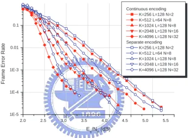
(11) 4.7.3. Separate and continuous encoding . . . . . . . . . . . . . . . . . . 101. 5 Stream-oriented inter-block permutation interleaver. 106. 5.1. Stream-oriented IBP interleaver and the associated encoding storage . . . 107. 5.2. Stream-oriented IBPTC encoding and the associated storage . . . . . . . 108. 5.3. Pipeline decoder and the associated message-passing on the factor graph 110. 5.4. Bound and constraints modification for S-IBP interleaver . . . . . . . . . 111. 5.5. Codeword weight upper-bounds of stream-oriented IBPTC . . . . . . . . 114 5.5.1. The upper-bound for weight-2 input sequences . . . . . . . . . . . 116. 5.5.2. The upper-bound for weight-4 input sequences . . . . . . . . . . . 118. 5.5.3. Interleaving gain comparison . . . . . . . . . . . . . . . . . . . . . 121. 5.6. Stream-oriented IBP . . . . . . . . . . . . . . . . . . . . . . . . . . . . . 121. 5.7. Modified semi-random interleaver . . . . . . . . . . . . . . . . . . . . . . 121. 5.8. Simulation Results . . . . . . . . . . . . . . . . . . . . . . . . . . . . . . 123 5.8.1. Covariance and convergence behavior . . . . . . . . . . . . . . . . 124. 5.8.2. Error probability performance . . . . . . . . . . . . . . . . . . . . 126. 6 Dynamic IBPTC decoder and stopping criteria 6.1. 6.2. 6.3. 134. IBP turbo coding system with stopping mechanism . . . . . . . . . . . . 135 6.1.1. System model . . . . . . . . . . . . . . . . . . . . . . . . . . . . . 135. 6.1.2. Iterative decoder with variable termination time . . . . . . . . . . 137. 6.1.3. Graphical representation of an IBPTC and CRC codes . . . . . . 141. Dynamic decoder and the associated issues . . . . . . . . . . . . . . . . . 141 6.2.1. Dynamic decoder . . . . . . . . . . . . . . . . . . . . . . . . . . . 142. 6.2.2. Decoding delay . . . . . . . . . . . . . . . . . . . . . . . . . . . . 143. 6.2.3. Memory contention and decoding schedule for multiple ADUs . . 146. 6.2.4. Memory management . . . . . . . . . . . . . . . . . . . . . . . . . 148. Multiple-round stopping tests . . . . . . . . . . . . . . . . . . . . . . . . 152. ix.

(12) 6.4. 6.3.1. A general algorithm . . . . . . . . . . . . . . . . . . . . . . . . . . 153. 6.3.2. T1.m: the m-round CRCST . . . . . . . . . . . . . . . . . . . . . 154. 6.3.3. T2.m: the m-round SCST . . . . . . . . . . . . . . . . . . . . . . 155. 6.3.4. T3.m: the m-round hybrid stopping test (MR-HST) . . . . . . . . 156. 6.3.5. Genie stopping test . . . . . . . . . . . . . . . . . . . . . . . . . . 156. Simulation results . . . . . . . . . . . . . . . . . . . . . . . . . . . . . . . 157. 7 Multi-stage factor graph 7.1. 7.2. 163. Multi-stage factor graph . . . . . . . . . . . . . . . . . . . . . . . . . . . 164 7.1.1. LDPC code . . . . . . . . . . . . . . . . . . . . . . . . . . . . . . 165. 7.1.2. S-IBPTC . . . . . . . . . . . . . . . . . . . . . . . . . . . . . . . 169. Multi-stage factor sub-graph . . . . . . . . . . . . . . . . . . . . . . . . . 172 7.2.1. LDPC code . . . . . . . . . . . . . . . . . . . . . . . . . . . . . . 173. 7.2.2. S-IBPTC . . . . . . . . . . . . . . . . . . . . . . . . . . . . . . . 174. 7.2.3. Discussion . . . . . . . . . . . . . . . . . . . . . . . . . . . . . . . 175. 7.3. Causal multi-stage sub-graph . . . . . . . . . . . . . . . . . . . . . . . . 176. 7.4. A memory-saving schedule for S-IBPTC . . . . . . . . . . . . . . . . . . 179. 7.5. Simulation results . . . . . . . . . . . . . . . . . . . . . . . . . . . . . . . 181. 8 Conclusions. 183. A Proof of Lemma 3.6. 185. B Proof of Lemma 3.7. 187. C Proof of Theorem 3.3. 188. D Proof of Theorem 5.10. 190. E Puncturing Patterns. 197. x.

(13) Bibliography. 198. About the Author. 217. xi.

(14) List of Figures 1.1. An inherent IBP structure can be found in most practical interleavers. . .. 2.1. (a) The block diagram of a generic digital communication system; (b) the. 10. block diagram of a simplified channel model; (c) the block diagram of a discrete memoryless channel model. . . . . . . . . . . . . . . . . . . . . .. 14. 2.2. (a) The controller canonical form; (b) The observer canonical form. . . .. 18. 2.3. (a) The encoder associated with G(D) = (D + D2 , 1 + D + D2 ); (b) state diagram; (c) trellis segment. . . . . . . . . . . . . . . . . . . . . . . . . .. 2.4. 21. (a) The block diagram of turbo code encoder; (b) the block diagram of turbo code decoder. . . . . . . . . . . . . . . . . . . . . . . . . . . . . . .. 30. 2.5. An example of a turbo code factor graph. . . . . . . . . . . . . . . . . . .. 34. 2.6. The parallel turbo decoder architecture. . . . . . . . . . . . . . . . . . .. 38. 2.7. a) The block diagram of a decoding module for one iteration; (b) The block diagram of the pipeline decoder. . . . . . . . . . . . . . . . . . . .. 39. 3.1. The block diagram of inter-block permutation turbo code encoder. . . . .. 41. 3.2. (a) Inter-block permutation interleaver; (b) Reversed inter-block permutation interleaver (c) Sandwich inter-block permutation interleaver. . . .. 43. 3.3. Partition of equivalence classes; L = 66, Tc = 9. . . . . . . . . . . . . . .. 56. 3.4. Set mapping; N1 = 3, N2 = 6 and n = 8. . . . . . . . . . . . . . . . . . .. 59. 3.5. The weight 2 lower bound for the Scrambling function. 1+D2 . 1+D+D2. 3.6. The weight 2 lower bound for the Scrambling function. 1+D+D3 . 1+D2 +D3. xii. . . . . . . . . . . .. 61 62.

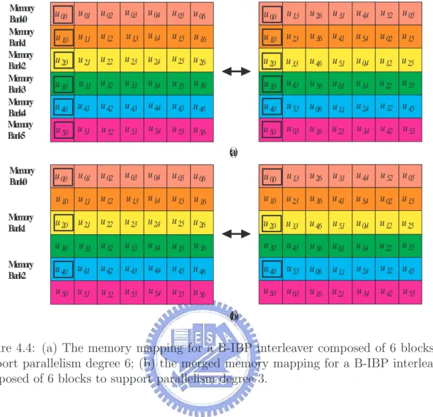
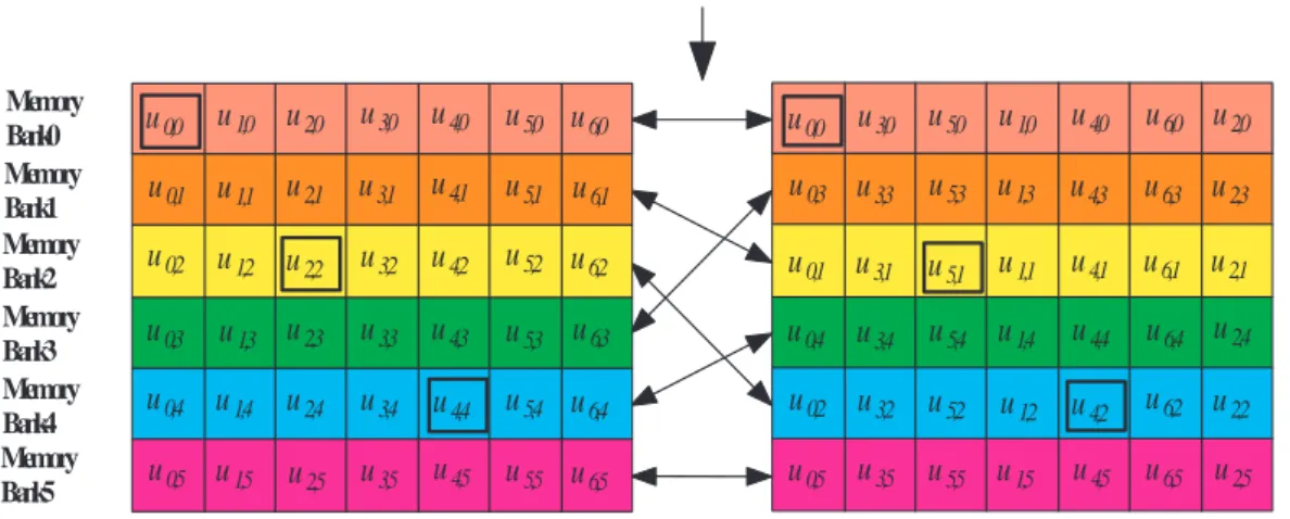
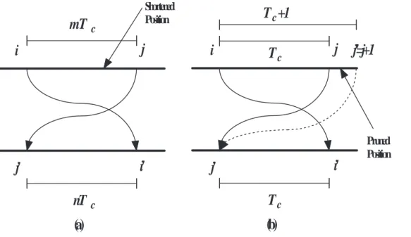
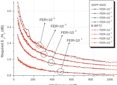
(15) 1+D2 +D3 +D4 . 1+D+D4. . . .. 3.7. The weight 2 lower bound for the Scrambling function. 4.1. (a) The block diagram of the parallel turbo decoder architecture with. 62. parallelism degree 4; (b) memory contention; (c) memory contention-free.. 65. 4.2. The block diagram of a block-oriented IBPTC encoder. . . . . . . . . . .. 67. 4.3. An example of block-oriented IBP interleaving. . . . . . . . . . . . . . . .. 68. 4.4. (a) The memory mapping for a B-IBP interleaver composed of 6 blocks to support parallelism degree 6; (b) the merged memory mapping for a B-IBP interleaver composed of 6 blocks to support parallelism degree 3. .. 4.5. The reversed memory mapping for the B-IBP interleaver composed of 7 blocks to support parallelism degree 3. . . . . . . . . . . . . . . . . . . .. 4.6. 4.9. 76. (a) Two connected trellis segments referring to Fig. 2.3 (c); (b) The merged trellis segment for the radix-4 APP decoder. . . . . . . . . . . . .. 4.8. 76. The block diagram of the asymmetric parallel turbo decoder architecture with 4 memory banks and 3 APP decoders. . . . . . . . . . . . . . . . .. 4.7. 74. 81. An example of butterfly network-oriented turbo code decoder architecture with parallelism degree 8. . . . . . . . . . . . . . . . . . . . . . . . . . .. 84. Multiple steams decoding. . . . . . . . . . . . . . . . . . . . . . . . . . .. 86. 4.10 An example of barrier shifter network-oriented turbo code decoder architecture with parallelism degree 8. . . . . . . . . . . . . . . . . . . . . . . 4.11 Weight-2 and 4 error events for a turbo code.. . . . . . . . . . . . . . . .. 89 92. 4.12 Influence of the weight-2 error events for both shortening and pruning strategy. . . . . . . . . . . . . . . . . . . . . . . . . . . . . . . . . . . . .. 93. 4.13 Frame error rate comparison for our implementation. . . . . . . . . . . .. 97. 4.14 Chip photo [112]. . . . . . . . . . . . . . . . . . . . . . . . . . . . . . . .. 98. 4.15 The B-IBP interleaver vs. 3GPP Rel’6 interleaver with the length ranging from 40 to 1000 bits. . . . . . . . . . . . . . . . . . . . . . . . . . . . . . 100. xiii.

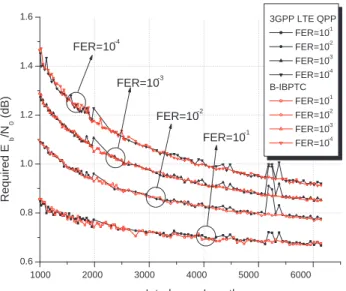
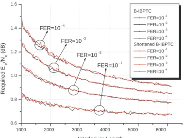
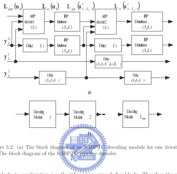
(16) 4.16 The B-IBP interleaver vs. 3GPP Rel’6 interleaver with the length ranging from 1000 to 6144 bits. . . . . . . . . . . . . . . . . . . . . . . . . . . . . 101 4.17 The B-IBP interleaver vs. 3GPP LTE QPP interleaver with the length ranging from 40 to 1000 bits. . . . . . . . . . . . . . . . . . . . . . . . . . 102 4.18 The B-IBP interleaver vs. 3GPP LTE QPP interleaver with the length ranging from 1000 to 6144 bits. . . . . . . . . . . . . . . . . . . . . . . . 103 4.19 The shortening and puncturing effect for the B-IBP interleaver with the length ranging from 40 to 1000 bits. . . . . . . . . . . . . . . . . . . . . . 103 4.20 The shortening and puncturing effect for the B-IBP interleaver with the length ranging from 1000 to 6144 bits. . . . . . . . . . . . . . . . . . . . 104 4.21 The comparison between the separate and continuous encoding for code rate 1/2. . . . . . . . . . . . . . . . . . . . . . . . . . . . . . . . . . . . . 104 4.22 The comparison between the separate and continuous encoding for code rate 3/4. . . . . . . . . . . . . . . . . . . . . . . . . . . . . . . . . . . . . 105 5.1. (a) Conventional inter-block permutation (S = 1); (b) Storage saving inter-block permutation (S = 1). . . . . . . . . . . . . . . . . . . . . . . . 109. 5.2. (a) The block diagram of an S-IBPTC decoding module for one iteration; (b) The block diagram of the S-IBPTC pipeline decoder. . . . . . . . . . 111. 5.3. The time diagram of the pipeline decoder with 4 APP decoders or Imax = 2.112. 5.4. A factor graph representation for an S-IBPTC encoded system with the S-IBP span 1. . . . . . . . . . . . . . . . . . . . . . . . . . . . . . . . . . 113. 5.5. Partition of equivalence classes into subsets; L = 68, Λ = 27, Tc = Ts = 3. 117. 5.6. Pre- and post-interleaving nonzero coordinate distributions of weight-4 input sequences that result in low-weight S-IBPTC codewords. . . . . . . 119. 5.7. Covariance between a priori information input and extrinsic information output. . . . . . . . . . . . . . . . . . . . . . . . . . . . . . . . . . . . . . 125. xiv.

(17) 5.8. Exit chart performance of the S-IBPTC and the classic TC at different Eb /N0 ’s. . . . . . . . . . . . . . . . . . . . . . . . . . . . . . . . . . . . . 126. 5.9. SNR evolution chart behavior of the S-IBPTC and the classic TC at different Eb /N0 ’s. . . . . . . . . . . . . . . . . . . . . . . . . . . . . . . . 127. 5.10 A comparison of covariance of bit-level and symbol-level IBP. . . . . . . . 128 5.11 BER performance of the S-IBPTCs with interleaver delay ≈ 800, block size L = 402 and interleaver span S = 1 and the classic TCs with block sizes L = 400, 800.. . . . . . . . . . . . . . . . . . . . . . . . . . . . . . . 129. 5.12 BER performance of the S-IBPTCs with interleaver delay ≈ 800, block size L = 265 and interleaver span S = 2 and the the classic TCs with block sizes L = 400, 800 are also given. . . . . . . . . . . . . . . . . . . . 130 5.13 BER performance of S-IBPTCs and the classic TC with interleaver delay 1320 and the 3GPP interleaver. . . . . . . . . . . . . . . . . . . . . . . . 131 5.14 BER performance of S=IBPTCs and the classic TC with interleaver delay 1320 and the modified semi-random interleaver. . . . . . . . . . . . . . . 132 5.15 Influence of the interleaver span on the BER performance for various SIBPTCs with interleaver delay 1320. . . . . . . . . . . . . . . . . . . . . 132 5.16 BER comparison of S-IBPTCs and the 3GPP defined turbo code of various block sizes. . . . . . . . . . . . . . . . . . . . . . . . . . . . . . . . . 133 5.17 A comparison of S-IBPDTC applying bit-level and symbol-level IBP with DTC using both Log-MAP and MAX Log-MAP APP decoders. . . . . . 133 6.1. The block diagram of the proposed VTT-APP decoder applied IBP turbo coding system.. 6.2. . . . . . . . . . . . . . . . . . . . . . . . . . . . . . . . . 136. A graph representation for a CRC and S-IBPTC encoded system with interleaving span S = 1. . . . . . . . . . . . . . . . . . . . . . . . . . . . 138. 6.3. The block diagram of IBPTC dynamic decoder. . . . . . . . . . . . . . . 142. xv.

(18) 6.4. A comparison of exemplary decoding schedules for classic TC and SIBPTC when decoding 7 blocks with 2 iterations (four decoding rounds). The numbers in the two rectangular grid-like tables represent the order the APP decoder performs decoding. . . . . . . . . . . . . . . . . . . . . 144. 6.5. A multiple zigzag decoding schedule for an S-IBPTC with the span S = 1. 147. 6.6. A joint memory management and IBPTC decoding procedure. . . . . . . 150. 6.7. Flow chart of a general m-round stopping test. . . . . . . . . . . . . . . . 155. 6.8. Block error rate performance of various stopping tests; no memory constraint; Dmax = 30 DRs. . . . . . . . . . . . . . . . . . . . . . . . . . . . 158. 6.9. Average APP DR performance of various stopping tests; Dmax = 30 DRs, no memory constraint. . . . . . . . . . . . . . . . . . . . . . . . . . . . . 159. 6.10 The effect of memory constraint and management on the block error rate performance. Curves labelled with infinite memory are obtained by assuming no memory constraint; “fixed DRs” implies that no early stopping test is involved.. . . . . . . . . . . . . . . . . . . . . . . . . . . . . . . . 160. 6.11 Average APP DR performance for various decoding schemes and conditions. Curves labelled with infinite memory are obtained by assuming no memory constraint; “fixed DRs” means no early-stopping condition is imposed. . . . . . . . . . . . . . . . . . . . . . . . . . . . . . . . . . . . . 161 6.12 Block error rate performance of a classic TC using various STs; L = 800 bits and Dmax = 30 DRs. . . . . . . . . . . . . . . . . . . . . . . . . . . . 162 6.13 The effect of various STs on the average APP DR performance of a classic TC with L = 800 and Dmax = 30 DRs. . . . . . . . . . . . . . . . . . . . 162 7.1. (a) Factor graph representation of an LDPC code; (b) the grouped factor graph; (c) node grouping.. . . . . . . . . . . . . . . . . . . . . . . . . . . 167. 7.2. Multi-stage factor graph for conventional BP algorithm. . . . . . . . . . . 168. 7.3. Multi-stage factor graph for horizontal-shuffled BP. . . . . . . . . . . . . 169 xvi.

(19) 7.4. Multi-stage factor graph for the new scheduled BP which reduces cycle effect. . . . . . . . . . . . . . . . . . . . . . . . . . . . . . . . . . . . . . 170. 7.5. Factor graph representation of a CRC- and S-IBPTC-coded communication link. . . . . . . . . . . . . . . . . . . . . . . . . . . . . . . . . . . . . 171. 7.6. (a) Node grouping; (b) grouped factor graph. . . . . . . . . . . . . . . . . 172. 7.7. A multi-stage factor graph for the S-IBPTC pipeline decoding schedule. . 173. 7.8. A multi-stage factor graph for the new S-IBPTC decoding schedule. . . . 174. 7.9. (a) The multi-stage factor sub-graph associated with Fig. 7.9; (b) the multi-stage factor sub-graph associated with Fig. 7.3; (c) the multi-stage factor sub-graph associated with Fig. 7.4; (d) the initial multi-stage factor sub-graph associated with Fig. 7.4. . . . . . . . . . . . . . . . . . . . . . 175. 7.10 (a) The multi-stage factor sub-graph extracted from Fig. 7.7; (b) the multi-stage factor sub-graph extracted from Fig. 7.8. . . . . . . . . . . . 176 7.11 (a) The sub-graph of the MSFG shown in Fig. 7.7; (b) the sub-graph of the MSFG shown in Fig. 7.8; (c) the causal multi-stage sub-graph associated with the MSFG shown in Fig. 7.7; (d) the causal multi-stage sub-graph associated with the MSFG shown in Fig. 7.8. . . . . . . . . . . 177 7.12 (a) Padded virtual nodes retain the regularity of the CMSSG for the beginning nodes on the MSFG; (b) padded virtual nodes retain the regularity of the CMSSG for the last nodes on the MSFG. . . . . . . . . . . . . . . 178 7.13 A memory saving schedule for the S-IBPTC. . . . . . . . . . . . . . . . . 179 7.14 The beginning stages on the partial MSFG associated with Fig. 7.13. . . 180 7.15 BER performance as a function of SNR for three decoding schedules. . . 182 7.16 Average APP decoding round number performance as a function of SNR for three decoding schedules. . . . . . . . . . . . . . . . . . . . . . . . . . 182 E.1 Frame error rate comparison between regular and irregular puncturing patterns for code rate=3/4 3GPP Rel’6 turbo code. . . . . . . . . . . . . 199 xvii.

(20) E.2 Frame error rate comparison between regular and irregular puncturing patterns for code rate=3/4 B-IBPTC. . . . . . . . . . . . . . . . . . . . . 199 E.3 Frame error rate comparison between 3GPP Rel’6 turbo code and BIBPTC for code rate=3/4 irregular puncturing pattern. . . . . . . . . . . 200 E.4 Frame error rate comparison between regular and irregular puncturing patterns for code rate=4/5 3GPP Rel’6 turbo code. . . . . . . . . . . . . 200 E.5 Frame error rate comparison between regular and irregular puncturing patterns for code rate=4/5 B-IBPTC. . . . . . . . . . . . . . . . . . . . . 201 E.6 Frame error rate comparison between 3GPP Rel’6 turbo code and BIBPTC for code rate=4/5 irregular puncturing pattern. . . . . . . . . . . 201 E.7 Frame error rate comparison between regular and irregular puncturing patterns for code rate=8/9 3GPP Rel’6 turbo code. . . . . . . . . . . . . 202 E.8 Frame error rate comparison between regular and irregular puncturing patterns for code rate=8/9 B-IBPTC. . . . . . . . . . . . . . . . . . . . . 202 E.9 Frame error rate comparison between 3GPP Rel’6 turbo code and BIBPTC for code rate=8/9 irregular puncturing pattern. . . . . . . . . . . 203. xviii.

(21) List of Tables 3.1. (α, β) for some RSC codes. . . . . . . . . . . . . . . . . . . . . . . . . . .. 60. 4.1. Throughput and latency analysis for 8 APP decoders . . . . . . . . . . .. 87. 4.2. Throughput and latency analysis for 16 APP decoders . . . . . . . . . .. 88. 4.3. Parallelism degree corresponding to various data lengths K and the supported number of interleavers. . . . . . . . . . . . . . . . . . . . . . . . .. 94. 4.4. Butterfly B-IBP sequences and the corresponding generator polynomials. 95. 4.5. Double prime interleaver parameters . . . . . . . . . . . . . . . . . . . .. 96. 4.6. Comparison to different turbo decoder designs . . . . . . . . . . . . . . .. 99. 5.1. S-IBP Algorithm . . . . . . . . . . . . . . . . . . . . . . . . . . . . . . . 122. E.1 Puncturing patterns for code rate=3/4. . . . . . . . . . . . . . . . . . . . 198 E.2 Puncturing patterns for code rate=4/5. . . . . . . . . . . . . . . . . . . . 198 E.3 Puncturing patterns for code rate=8/9. . . . . . . . . . . . . . . . . . . . 198. xix.

(22) Glossary. 3GPP 3GPP LTE ADU APP ARP ASIC AWGN B-IBP B-IBPTC BCH BCJR BER BLER C-IBPTC CE CP CRC CRC-SC ST CRCST CMSSG D-IBPTC DWW DPSK DR DRP DSP DTC DVB-RCS DVB-RCT EXIT ESD FER IBP IBPTC. Third Generation Partnership Project Third Generation Partnership Project Long Term Evolution A Posteriori Probability Decoding Unit A Posteriori Probability Almost Regular Permutation Application Specific Integrated Circuit Additive White Gaussian Noise Block-Oriented Inter-Block Permutation Block-Oriented Inter-Block Permutation Turbo Code Bose-Chaudhuri-Hocquenghem Bahl-Cocke-Jelinek-Raviv Bit Error Rate Block Error Rate Continuous Inter-Block Permutation Turbo Code Cross Entropy Cyclic Prefix Cyclic Redundancy Check Cyclic Redundancy Check-Sign Check Stopping Test Cyclic Redundancy Check Stopping Test Causal Multi-Stage Sub-Graph Discontinuous Inter-Block Permutation Turbo Code Decoding Window Width Differential Phase Shift Keying Decoding Round Dithered Prime Permutation Digital Signal Processing Duo-Binary Turbo Code Digital Video Broadcast-Return Channel Satellite Digital Video Broadcast-Return Channel Terrestrial Extrinsic Information Transfer Extended Stopping Decision Frame Error Rate Inter-Block Permutation Inter-Block Permutation Turbo Code. xx.

(23) ID-BICM IN ISI LDPC Log-MAP MAP MAX Log-MAP MIMO MMSE MR-HST MRST MSFG MSFSG MU OFDM QAM QPP RDR RS RSC S-C-IBPTC S-IBP S-IBPDTC S-IBPTC S-TB-IBPTC S-TP-IBPTC SC SCST SNR SOVA SRID ST SV SVST SWAPP TB-IBPTC TC TCM TP-IBPTC VTT VTT-APP. Iterative Decoding Bit-Interleaved Coded Modulation Iteration Number Inter-Symbol Interference Low Density Parity Check Logarithmic Maximum a Posteriori Maximum a Posteriori Maximum Logarithmic Maximum a Posteriori Multiple Input Multiple Output Minimum Mean Square Error Multiple-Round Hybrid Stopping Test Multiple-Round Stopping Test Multi-Stage Factor Graph Multi-Stage Factor Sub-Graph Memory Unit Orthogonal Frequency Division Modulation Quadrature Amplitude Modulation Quadratic Permutation Polynomial Repeated Decoding Round Reed-Solomon Recursive Systematic Convolutional Code Stream-Oriented Continuous Inter-Block Permutation Turbo Code Stream-Oriented Inter-Block Permutation Stream-Oriented Inter-Block Permutation Duo-Binary Turbo Code Stream-Oriented Inter-Block Permutation Turbo Code Stream-Oriented Tail-Biting Inter-Block Permutation Turbo Code Stream-Oriented Tail-Padding Inter-Block Permutation Turbo Code Sign Check Sign Check stopping Test Signal to Noise Ratio Soft Output Viterbi Algorithm Single Round Interleaving Delay Stopping Test Soft Value Soft Value Stopping Test Sliding-Window a Posteriori Probability Tail-Biting Inter-Block Permutation Turbo Code Turbo Code Trellis Coded Modulation Tail-Padding Inter-Block Permutation Turbo Code Various Termination Time Various Termination Time-a Posteriori Probability. xxi.

(24) Chapter 1 Introduction The invention of turbo codes by Berrou et al. in the early 1990s [13] has ignited a revolution within the coding research community. The underlying turbo principle has since crossed the borderline of coding theory and made far-reaching impacts on various scientific disciplines like communications, computer science, statistics, physics and bioinformatics, to name just a few.. 1.1. Turbo decoding. The now classic turbo code is composed of two identical short recursive systematic convolutional codes and a random-like interleaver. A message sequence and its interleaved version are separately encoded by two component encoders and the resulting codeword consists of the original sequence (systematic part) and two parity sequences. Each parity sequence along with the systematic part or its interleaved version forms a conventional convolutional codeword. The original decoder proposed by Berrou et al. has a serial structure with identical a posteriori probability (APP) decoders. Maximum a posteriori probability (MAP) algorithm [8] is iteratively applied to decode each convolutional code and produce reliability estimates about the systematic bits. The reliability estimate, which is universally called extrinsic information now, generated by one APP decoder is interleaved or de-interleaved and then passed on to the other APP decoder for use as the a priori information needed 1.

(25) in its MAP decoding. Such a turbo-like iterative feedback decoding procedure divides the formidable task of maximum likelihood (ML) decoding of the complete codeword into much simpler subtasks of computing the log-likelihood ratio (extrinsic information) associated with each systematic bit locally and exchanging this information between each other. It turns out this turbo decoding scheme is very effective and the resulting performance comes very close to that of the corresponding ML decoder. Because of its outstanding performance and moderate hardware complexity, the class of turbo codes has found its way into industrial standards like 3GPP [1, 2, 3], IEEE 802.16 [56], DVB-RCS/RCT [37, 38], etc. The turbo decoding process was formulated by Hagenauer et al. [50] as a softin soft-out inference process that accepts soft inputs–including a priori and channel values–and generate soft outputs which consists of the a priori and channel values and the extrinsic values. The extrinsic value is then used as an a priori value for the ensuing decoding round. The turbo decoding procedure and the way the extrinsic information is passed is often referred to as the turbo principle. This principle has been applied to construct and decode serial concatenated convolutional codes [10], turbo TCMs [84], turbo BCH codes [109], turbo product codes or block turbo codes (BTCs) [81, 80], turbo Reed-Muller codes [109], and asymmetric turbo codes [91] (which has different component convolutional codes and offers better performance). Replacing the inner code of a serial concatenated coding system by a differential phase shift keying modulator or signal mapper, one obtains turbo DPSK [53] or iterative-decoded bit-interleaved coded modulation (ID-BICM) [72, 71]. Modelling a channel with memory as a linear FIR filter or equivalently a finite-state machine so that the combination of coding and channel effects becomes a serial concatenated system with the channel performing inner coding, one can detect the received signal by iteratively equalizing the channel effect and then decoding, resulting in turbo equalization [36], turbo space-time processing [6] and turbo (iterative) MIMO detection [7], [19]. By using more than two component codes and. 2.

(26) multiple interleavers, Boutillon and Gnaeding [22] investigated the structure of multiple turbo codes. Replacing the one-to-one permutation function by a many-to-one mapping, Frey and MacKay [45] proposed the so-called irregular turbo codes. stream-oriented turbo code was proposed by Hall [51], a pipeline architecture was studied in [101].. 1.2. Performance analysis and graph codes. The reasons for the extraordinary performance of the TC, although unclear initially, has been unraveled through many excellent and intensive research efforts. Benedetto and Montorsi [9] showed that the iterative (turbo) decoding algorithm is capable of achieving near-ML performance and the error rate performance improves as the interleaver length increases. They also found that the interleaver length can be traded with component code’s complexity and that the number of nearest neighbors rather than the minimum distance dominates the performance, at least when SNR is small. Perez et al. [74] analyzed the TC ensemble (over all possible interleavers), examined the code’s distance spectrum and came to a similar conclusion that the error floor occurs at moderate to high SNR is due to the relatively small free distance of the component code and its excellent performance at low SNR is resulted from spectrum thinning. They found that the low weight codewords, in particular those generated by weight-2 input sequences, dominate the error rate performance especially at the error floor region. The convergence behavior of the turbo decoding algorithm was analyzed by Richardson [82, 83] from a geometric viewpoint. He also suggested a density evolution approach to compute the thresholds for low density parity check (LDPC) codes. The concept of density evolution was later extended to be applicable to turbo codes [82]. The analysis of El Gamal and Hammons [39] is based on the fact that the extrinsic values at the output of an APP decoder is well approximated by Gaussian random variables and channel values are also Gaussian distributed when the only noise source is AWGN–an observation first noticed by Wiberg [108]. As a Gaussian distribution is completely char3.

(27) acterized by its first two moments, the density evolution information can be replaced by SNR transfer. Both [39] and Divsalar et al. [34] use similar SNR measures to study the convergence of turbo decoders. Extrinsic information transfer (EXIT) chart [27, 28] proposed by ten Brink plots the increase of extrinsic information through the component decoders based on the measure of mutual information between extrinsic information and the associated information symbol or code symbol. A special class of graphs called factor graphs [60, 42] can be used to describe the behavior and structure of a turbo-like algorithm. A factor graph decomposes the algorithmic structure into function nodes and variable nodes with edges connecting these function nodes. McEliece et al. [66] discovered the connection between the turbo decoding algorithm and the belief propagation (BP) algorithm in artificial intelligence. The graphic and BP interpretations of the turbo decoder have great impacts and opened new arenas on many fronts: new decoding algorithms, schedules and new (graph) codes were proposed, a unified view on iterative decoding algorithm, Kalman filter, the forwardbackward, Baum-Welch, and Viterbi algorithms become possible, connection between turbo codes and LDPC codes was established, that amongst coding theory, statistical inference, physics was exploited to the benefits of all involved research communities .. 1.3. Low latency/high performance interleavers. The role played by the interleaver in determining the decoding latency, weight distributions and performance of a TC is of critical importance. A TC usually employs a block-oriented interleaving so that the message-passing process associated with an iterative decoder is confined to proceed within a block. The performance of such a TC improves as the block size increases. This is in part due to the fact that the range (interleaving length) of the extrinsic information collected for decoding increases accordingly. But the interleaving size along with the number of iterations are the dominant factors that determine the decoding latency and complexity which, in turn, are often the main 4.

(28) concerns that precluding the adoptability of such codes in high rate communication or storage applications. The semi-random interleaver [44] increases the codeword weights corresponding to the weight-2 input sequences but not those for weight-4 input sequences. The code matching interleaver of [40] considers the influence of component codes and extended the optimization criterion to include the weight-4 input sequences, yielding performance superior to that based on a semi-random interleaver. The methods proposed in [54, 86] are based on the analysis of the correlation of extrinsic information resulted from cycles in the code graph. They design interleaving rules to reduce the cycle effect and obtain slightly-improved performance. A common shortcoming of these interleaver designs is their lack of an algebraic structure. A look-up table is therefore needed in implementation. Structural interleavers are now abundant: 3GPP Rel’99 and Rel’6 interleaver [1, 2], dithered relative prime interleaver [30, 31], dithered golden interleaver (DRP) [30], almost regular permutation (ARP) [12, 37, 38, 56], quadratic polynomial permutation (QPP) [90, 85, 92, 93, 3], to name the important ones. These interleavers are generated by few parameters and the corresponding storage requirements are moderate. Besides a simple algebraic structure, we notice a recent trend indicating that high throughput (¿ 100 Mbps) turbo decoders [3, 56] are in great demand. The low latency/high throughput applications require that the interleaver be such that the corresponding turbo code is parallel decodable. Some design issues arise because of this requirement. Firstly, we notice that since a parallel decoder consists of many APP decoders, each responsible for decoding a (non-overlapping) part of the incoming block, these decoders would simultaneously and periodically access the memory banks that store the extrinsic information and channel values through hardwires. Thus the parallel decodable requirement implies that the interleaver structure must be memory contentionfree and allow simple interconnecting network for hardwire routing. Next, practical. 5.

(29) system design concerns call for flexible degrees of parallelism and arbitrary continuous interleaving length so that one has flexible choice on both the number of APP decoders and the frame (packet) size. Random interleavers, although offer satisfactory error rate performance, incur serious memory contention. Implementing temporary memory buffer [49] to avoid memory contention is a viable solution but the storage grows linearly with the number of APP decoders. Resolving the contention by a sophisticated memory mapping function [95] requires a table for each interleaving length. The table requires memory storage for addressing and memory control which results in extra hardware complexity. A large number of interleaving lengths thus need many memory addressing tables and causes increased hardware complexity. New industrial standards such as 3GPP [1, 2, 3], DVBRCS/RCT [37, 38], IEEE 802.16 [56] do not favor this approach for the demand of large number of interleavers and low complexity memory addressing. A variable length interleaver structure that resolves memory contention with on-fly generated memory mapping function is an efficient and welcome approach. Some of the existing interleavers like the DRP, ARP and QPP do have simple algebraic structures and possess the memory contention-free property, the DRP even yields a minimum distance that is close to the known upper bound, resulting in outstanding performance especially for frame error rate below 10−6 . However, none of them takes into account the other requirements which are of concern mainly to the circuit design community. A fully-connected network can be used but the complexity grows in proportion to the square of the parallelism degree. The average routing length also increases, bringing about longer routing latency and higher power consumption. The network configuration is close related to the interleaving/deinterleaving rule used. Irregular routing control should be avoid as it necessitates complex controlling signalling. For more detailed discussion on the routing network complexity and network configuration signalling please. 6.

(30) refer to [78, 68, 67, 33]. Memory addressing also depends on interleaver design. [70, 95, 96] have investigated the memory addressing and permutation table storage problems. 3GPP Rel’99 and Rel’6 [1, 2] applies the prime interleaver as the intra-row permutation and this interleaver needs storage for the permutation table of each row. The intramemory bank addressing induces storage complexity if the table can not be generated on-fly. Therefore 3GPP LTE QPP [3] avoids the storage and replaces the interleaver. Popular hardware-friendly designs that avoids the above-mentioned storage requirement ARP [12, 37, 38, 56] and QPP [90, 85, 92, 93, 3]. Some parallelization methods are suggested in [49, 20, 98, 97].. 1.4. Statement of purpose: main contributions. The above discussion shows designing the interleaver for a TC for wireless applications has to consider both error rate performance and hardware/memory complexity. The main purpose of this thesis is to present a systematic and unified interleaver design flow and guideline that enable one to construct an interleaver of arbitrary practical lengths which not only meet all the above requirements but also guarantee little or no performance loss with respect to the that achievable by the best known code of the same or comparable interleaving lengths. To distinguish the TC without any constraints and the TC applying out interleaver, we refer the former class as the classic TC. The structure we propose is called inter-block permutation (IBP) interleaver. The IBP technique can be regarded as a simple way to build a larger interleaver based on smaller interleavers. It performs an extra inter-block permutation on those blocks that have already been interleaved by intra-block permutation. As the interleaver along with the component code determines the structure of classic TC, the concept of IBP interleaver is also similar to Tanner’s approach for constructing a large (long) code with small codes. The proposed interleaver structure is general enough to encompass all known important interleavers as special cases yet viable for generating new solutions. 7.

(31) We summarize the main contributions of our work documented in this thesis as follows. 1. We present a unified approach and design flow to build interleavers that not only have good distance properties but also meet all the major implementation requirements for high throughput turbo decoders. More specifically, the resulting interleaver structure (i) is maximum memory contention-free, (ii) allows low complexity routing network structure and simple signalling circuits, (iii) offers flexible choice in the degrees of parallelism, (iv) is easily tailored to serve the continuous interleaving length requirement, (v) supports the high-radix APP decoder structure and (v) includes all existing good interleavers as its subclasses. 2. For a stream-oriented application, our technique overcomes the dilemma between increasing the range of message exchange and extrinsic information collection and reducing the interleaving size (and therefore the decoding delay). It outperforms classic TCs with the same decoding delay and offers new design choices and tradeoffs that are unavailable for classic TC design. 3. We derive codeword weight bounds for weight-2 and weight-4 input sequences. More importantly, we use these bounds and computer simulations to prove that the advantages mentioned in 1-2 are achieved with little or no loss in error rate performance. 4. We present a dynamic corporative pipelined decoder structure that incorporate an efficient memory manager and a class of highly reliable early-stopping rules. The proposed decoder structure gives improved performance with reduced latency and memory requirement. 5. For non-parallel decoding, the IBP interleaver is still capable of reducing the decoding latency while maintaining satisfactory performance.. 8.

(32) 6. A graphic tool called multistage factor graphs is developed to analyze the behavior of parallel and pipelined decoding schedules. It is applied to design a new pipelined decoding schedule with reduced memory requirement and can also be used to design better schedule for decoding LDPC codes.. 1.5. Existing interleavers as instances of IBP interleaver. For a classic TC using an IBP interleaver, the encoder partitions the incoming data sequence into L-bit blocks upon which the IBP interleaver performs intra-block and then inter-block permutations. For example, the IBP interleaver may move contents of a block either to coordinates within the same block or to its 2S immediate neighboring blocks so that the IBP-interleaved contents of a block are spread over a range of 2S + 1 blocks centered at the original block. Such an IBP interleaver is said to have the (left or right) IBP span S. For any reasonable good interleaver of size N , partitioning each N -bit group into L = ⌊N/W ⌋-bit blocks immediately transforms the interleaving rule into an IBP structure like that shown in Fig. 1.1. Such a structure can also be found in other codes such as product codes. Consequently, all classic TCs and product codes can be regarded as subclasses of inter-block permutation turbo codes (IBPTCs). There are, however, two major distinctions between classic TCs and most other subclasses of IBPTCs. Firstly, for a classic TC with an interleaving length of W blocks, encoding within each disjoint group of W consecutive blocks is continuous across blocks while a product code encodes each row (column) separately (discontinuously). More specifically, the product code encoder divides information stream into multiple blocks and independently encodes each block. In general, the class of IBPTCs can encode each block either separately or continuously. Secondly, an interleaver used in a classic TC, after the above virtual regular partition, usually yields a non-regular local interleaving structure, i.e., the interleaving. 9.

(33) Pre-Permutation. 1. 2. 4. 3. b 1,1. b 1,2. b 1,3. b 1,4. b 2,1. b 2,2. b 2,3. b 2,4. b 3,1. b 3,2. b 3,3. b 3,4. b 4,1. b 4,2. b 4,3. b 4,4. b 1,4. b 2,1. b 3,2. b 4,3. b 2,4. b 1,1. b 4,2. b 3,3. b 3,4. b 4,1. b 1,2. b 2,3. b 4,4. b 3,1. b 2,2. b 1,3. 1. 2. 3. 4. Post-Permutation Figure 1.1: An inherent IBP structure can be found in most practical interleavers.. relation between a block and other blocks in the same group does not follow the same permutation rule. In contrast, product codes and the proposed IBPTCs have much more regular local interleaving structures. An appropriate regular local interleaving (and deinterleaving) structure makes implementation easier and, as mentioned before, provides properties that are useful for parallel decoding, e.g., (memory access) contention-free and simple routing requirement. Moreover, with or without parallel decoding, as the examples in Section 6.2 show, it also results in reduced decoding delay. Regular (identical) local interleaving structure supports large range of interleavers, makes the resulting IBP interleaver expandable and minimize the associated implementation cost, e.g. 3GPP LTE QPP [3], IEEE 802.16 [56].. 1.6. Overview of chapters. In order that this thesis be self-contained we provide major background material related to our work in Chapter 2. Two fundamental guidelines are provided in Chapter 3 for constructing IBP interleavers with good distance and maximum contention free properties. The first rule demands that the IBP rule be block-invariant and identical intra-block permutation e used. The second rule implies that the permutation should be periodic within its span. Following these and other minor guidelines we are able to. 10.

(34) construct interleavers that meet most of the hardware requirements while maintaining good distance properties. Searching for large range of interleaving lengths also become easier. We divide the class of IBP interleavers into block-oriented IBP (B-IBP) interleaver and stream-oriented IBP (S-IBP) interleaver. The B-IBP interleavers are treated in Chapter 4 while Chapter 5 deals with the stream-oriented IBP (S-IBP) interleavers. The B-IBP interleavers include popular interleavers such as the ARP and QPP and usually have hardware constraints more stringent than those on stream ones. Encoding variable information lengths with the same hardware architecture. We suggest simple memory mapping functions that support flexible choices in the number of memory banks and APP decoders. An alternate decomposition of an IBP rule called reverse IBP manner offers additional flexibility. In order to support the high-radix APP decoder and the generalized maximum memory contention-free property, we impose two constraints on the intrablock permutation and obtain simple and easily generated memory mapping functions. Our network-oriented design allows low complexity butterfly network and simple routing control signalling. To deal with variable message lengths without throughput loss, a shortening and puncturing algorithm is proposed to maintain both performance and hardware implementation edge. We provide an interleaver design with the interleaving length ranging from 40 to 6144 bits. A VLSI implementation example based on this design with a specific interleaving length of 4096 bits is also given. We prove that our S-IBP interleaver construction gives larger codeword weight upperbounds for the weight-2 and weight-4 input sequences than those of classic TCs with the same interleaver latency. Our S-IBP interleaver is well suited to pipeline decoder architectures [101]. To improve both hardware/memory efficiency and error rate performance we propose a dynamic decoder architecture which includes a memory manager and an early-stopping mechanism. The decoder also admits new decoding schedules and offers trade-off between throughput and hardware/memory complexity.. 11.

(35) In Chapters 6 we discuss issues concerning the pipelined decoders. Early-stopping in iterative decoding is an critical and very practical issue. Regarding the iterative decoding as an instance of sequential decision processes, early-stopping reduces the number of iterations (and thus the computation complexity/power) at high SNR without performance loss at low SNR. CRC code, sign check, soft value (cross entropy) are some of the more popular stopping schemes [50, 88, 65, 4]. The CRC code offers more reliable stopping decision than other schemes do at the cost of increased overhead and reduced bandwidth efficiency. The proposed multiple-round stopping mechanism enhances the stopping reliability with a smaller overhead, leading to the improved latency and error rate performance. Judicial design of decoding schedules is crucial for the parallel or pipeline turbo decoding. Conventional factor graphs are incapable of describing such decoding schedules for turbo codes and LDPC codes. In Chapter 7, we develop a new graphic tool called the multi-stage factor graphs to describe the the time-evolving message-passing and evaluate the performance of various decoding schedules for the parallel and pipeline decoders. A good decoding schedule is important in rendering satisfactory performance, e.g., the horizontal shuffled belief propagation algorithm [63] outperforms conventional belief propagation algorithm [60] in terms of the number of iterations required to achieve a desired error rate performance. Multi-stage factor graphs can be used to show the cycle effect and design new decoding schedule to avoid short cycles. We propose a novel decoding schedule for a stream-oriented IBPTC that requires much less memory storage and slightly increased computation but yields similar error rate performance. Finally, in Chapter 8 we summarize the main results of our work.. 12.

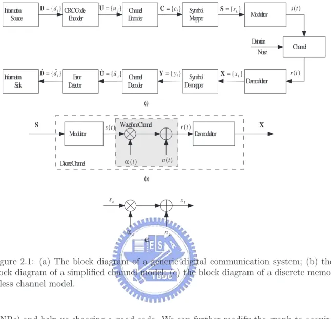
(36) Chapter 2 Fundamentals This chapter provides the backgrounds of this thesis. Channel coding embedded in a digital communication system [79] overcomes channel impairments, e.g. thermal noise, multi-path fading, etc. Turbo code [13] is an important candidate among these channel coding schemes. This code possesses better error rate performance comparing with the convolutional code with constraint length 41 [79] and can apply iterative decoding algorithm with less complexity to achieve the performance comparing to the Viterbi algorithm. The algorithm adopts maximum a posteriori (MAP) [8] algorithm to generate the extrinsic information for successive decoding as the a priori information and corrects errors after several iterations. In order to further reduce implementation complexity, many researches [50, 104] focus on the MAP algorithm simplification. Due to high performance with low computation complexity, many standards adopt turbo code, e.g. 3GPP Rel’99 and Rel’6 [1, 2], 3GPP LTE [3], DVB-RCS[37], DVB-RCT[38] etc. 3GPP LTE further requires the throughput exceeding 100Mbps and high throughput turbo decoder architecture becomes important topic; interleaver determines the implementation complexity and error rate performance. Theoretical performance analysis and codes characteristics are also of our interest. The factor graph [60, 42] expounds the structure of turbo code and some decoding algorithms are derived. Given the graph and decoding algorithm, the extrinsic information transfer (EXIT) chart [27, 28] and density evolution [34] explain the convergence behavior at various signal-to-noise ratios. 13.

(37) D = { d i } CRCCode. Information Source. Encoder. U = {u j } Channel Encoder. C = {c l }. Symbol Mapper. S = {s k }. Modulator. Distortion Noise Dˆ = {dˆi }. Information Sink. Error Detector. Uˆ = {uˆ j }. Y = { yl }. Channel Decoder. Symbol De-mapper. X = { xk }. s (t ). Channel. r (t ) De-modulator. (a). S Modulator. s (t ) WaveformChannel. α (t ). DiscreteChannel. X. r (t ) De-modulator. n (t ) (b). sk. xk. αk. (c). nk. Figure 2.1: (a) The block diagram of a generic digital communication system; (b) the block diagram of a simplified channel model; (c) the block diagram of a discrete memoryless channel model.. (SNRs) and help us choosing a good code. We can further modify the graph to acquire some distance bounds [75] which dominate the performance at high SNR. The following sections detail these implemental and theoretical backgrounds.. 2.1. Digital communication system. Fig. 2.1 (a) shows a generic digital communication system block diagram which includes three parts: 1) channel; 2) modulation, demodulation, mapper and de-mapper; 3) error correction and detection. Channel imposes non-ideal effects and distorts the modulated continuous waveform. Demodulator and de-mapper convert the distorted waveform into samples. Error correction recovers these samples and renders decoded 14.

(38) sequences. At last error detection verifies the correctness of decoded sequences. The following subsections will elaborate these three parts.. 2.1.1. Discrete memoryless channel model. A memoryless discrete channel model is characterized by a multiplicative distortion and a complex AWGN in Fig. 2.1 (c) and the received sample is xk = αk · zk + nk ,. (2.1). where A = {αk } and N = {nk } are identical independent Rayleigh (Rician) distributed random variables and complex Gaussian distributed random variables with C(0, N0 ) respectively. This model can replace channel, modulator and de-modulator in Fig. 2.1 (a). We combine modulator and demodulator to construct a discrete channel model which is shown in Fig. 2.1 (b). The thermal noise introduced by component devices can be modelled by the white Gaussian random process. As for the non-selective fading [79], we model fading process α(t) as a Rayleigh or Rician distributed random process and the value is almost invariant during each symbol period. As we apply a perfect channel interleaver between de-mapper and channel decoder, the correlation between adjacent modulation symbols diminishes after channel de-interleaving. Since the fading attenuation is uncorrelated and the thermal noise is white, the channel model can be further simplified as shown in Fig. 2.1 (c). Time domain dispersive multi-path fading effect introducing inter-symbol interference (ISI) also can be modelled by a memoryless discrete channel model as we apply orthogonal frequency division modulation (OFDM). OFDM applies a cyclic-prefix (CP) to maintain the longest path delay within the interval of the CP and we can sample a symbol period without interferences from other symbols and the ISI effect disappears. The frequency domain amplitude attenuation incurred from all paths can be modelled as a Rayleigh distributed random variable if there is no line of sight. If there is a line 15.

(39) of sight, the distribution is Rician distributed probability density function (pdf). The model in Fig. 2.1 (c) can be re-applied. The shadowing effect is a long-term effect and generally lasts more than one coding block. The effect can be modelled into the noise strength. Therefore the simplified memoryless discrete channel model properly covers most scenarios and this thesis will apply this model as our simulation assumption.. 2.1.2. Mapper and de-mapper. Mapper bridges channel encoder and modulator; de-mapper generates log-likelihood or log-likelihood ratio for code bits corresponding to a sample xk . Mapper maps n code bits into a modulated symbol Sm ∈ S by a mapping rule Φ : {bm,0 , bm,1 , . . . , bm,n−1 } → Sm ,. (2.2). where bi,j ∈ {0, 1} and |S| = 2n . Based on the mapping rule, de-mapper can apply maximum a posteriori (MAP) algorithm to generate a log-likelihood ratio of the tth code bit corresponding to the ith mapping bit as P. bm,i =0,bm,j ,j6=i. L(ct ) = log P. bm,i =1,bm,j ,j6=i. p(Sm |xk ). p(Sm |xk ). .. (2.3). L(ct ) is generally applied as yt to the following channel decoder. We further consider binary phase shift keying (BPSK) and the mapping rule is Φ:. ½. b0,0 = 0 → S0 = +1 . b1,0 = 1 → S1 = −1. (2.4). If P (ct = 0) = P (ct = 1) = 0.5 and the pdf of x given Sm and channel attenuation α is pX|Sm ,α (x|Sm , α) = √. 1 2πσ 2. exp−. (x−αSm )2 2σ 2. (2.5). with σ 2 = N0 /2, the log-likelihood ratio in eqn. (2.3) with k = t becomes L(ct ) = log. pX|S0 ,α (xt |S0 , αt ) p(S0 ) 4αt xt p(S0 |xt , αt ) = log + log = . p(S1 |xt , αt ) pX|S1 ,α (xt |S1 , αt ) p(S1 ) N0 16. (2.6).

(40) 2.1.3. Error control system. Error correction and detection are two main error control functions. Error correction function applies channel encoder and decoder to overcome channel distortion. Channel encoder generates coded sequence and channel decoder recovers the distorted sequence after channel corruption. Convolutional code, turbo code, LDPC code and Reed-Solomon code are now popular error correction codings. Error detection function generally relies on a cyclic redundancy check (CRC) code [109]. The CRC code encoder adds the error check parities behind information sequence and error detection function verifies the consistency between the decoded information sequence and parities. If the error verification fails, error control system discards decoded sequence or requests retransmission to render higher successful transmission probability. These two functions enhance and guarantee data transmission robustness via channel corruption.. 2.2. Convolutional code. Convolutional code encoder features simple structure which can be realized by finite shift registers and adders and is shown in Fig. 2.2. The codeword length is not stringently constrained comparing to the block code, e.g. RS code. The simple structure results in that the Viterbi algorithm [103, 41], soft decoding algorithm, is applicable and the resultant performance is better than the performance of RS code. In order to expound the code structure, we provide some mathematical notations at first.. 2.2.1. Mathematical notations. Denote by F2 [D] the ring of binary polynomials, where the power of D is nonnegative P∞ i and the coefficients are in Galois field GF (2), e.g. p(D) = i=0 pi D ∈ F2 [D] and. pi ∈ GF (2). Multiplication of two polynomials is a polynomial multiplication with coefficient operation performed under GF (2). Since the power of D is nonnegative, 1 is the only only element with its inverse and F2 [D] is a ring. 17.

(41) c. ... F1. F0. u. σ1 Q0. .... F2. σ2 Q1. σ3. Fm. σm. ... .... Q2. F m-1. Q m-1. Qm. F1. F0. ... (a). u. ... F m-1. Fm. σm Qm. σ m −1 Q m-1. .... F m-2. σ m−2. .... Q m-2. c. σ1. ... Q1. Q0. ... (b). Figure 2.2: (a) The controller canonical form; (b) The observer canonical form.. F2 (D) denotes the field of binary rational functions. Each element in F2 (D) is expressed by elements. x(D) , y(D). x(D) y(D). where each pair x(D), y(D) ∈ F2 [D] with y(D) 6= 0. Apparently all. ∈ F2 (D) are invertible and they form a field.. a×b We further denote by Fa×b 2 [D] and F2 (D) the a × b matrix of ring of binary polyno-. mials and the a×b matrix of the field of binary rational functions respectively. All entries a×b in X a×b (D) ∈ Fa×b (D) ∈ Fa×b 2 [D] and Y 2 (D) belong to F2 [D] and F2 (D) respectively.. If a = 1, the notations are simplified as Fb2 [D] and Fb2 (D).. 2.2.2. Encoder. A rate R = a/b convolutional code encodes input sequence u = u0 u1 u2 . . . and generates code sequence c = c0 c1 c2 . . . , where ui = {u1i , u2i , · · · , uai } and cj = {c1j , c2j , · · · , cbj }. 18.

(42) A sequence can be represented by the delay operator D (D-transform), and we have u(D) = u0 + u1 D + u2 D2 + · · · ,. (2.7). c(D) = c0 + c1 D + c2 D2 + · · · ,. (2.8). where u(D) ∈ Fa2 [D] and c(D) ∈ Fb2 [D]. The encoder input and output relation can be expressed as c(D) = u(D)G(D),. (2.9). where G(D) ∈ Fa×b 2 (D) is a transfer function matrix. The matrix has a form G(D) = Q−1 (D)F(D) = (Q0 + Q1 D + · · · + Qm Dm )−1 (F0 + F1 D + · · · + Fm Dm ),. (2.10). a×b where Q(D) ∈ Fa×a 2 [D] and F(D) ∈ F2 [D]. The polynomial matrix Q(D) is a diagonal. matrix with Q0 = Ia , Ia is an a × a identity matrix, i.e. the elements off the diagonal entries are zero. The matrix G(D) can be realized in the controller canonical form shown in Fig. 2.2 (a). Observer canonical form is another way in realizing transfer function matrix. We substitute eqn. (2.10) into eqn. (2.9) to render c(D) = u(D)(F0 + F1 D + · · · + Fm Dm ) + c(D)(Q1 D + · · · + Qm Dm ).. (2.11). Fig. 2.2 (b) shows the corresponding linear circuit which is the observer canonical form for a convolutional code encoder. Both controller and observer forms realize the transfer function matrix. From the above description, we give a formal definition of a convolutional code as follows. Definition 1 A code rate R = a/b (binary) convolutional code encoder over the field of rational functions F2 (D) is a linear mapping Φcc : Fa2 (D) → Fb2 (D) u(D) 7→ c(D) 19.

(43) which can be represented as c(D) = u(D)G(D), where G(D) ∈ Fa×b 2 (D) is an a × b transfer function matrix of rank a and c(D) is a code sequence generated from the information sequence u(D). Systematic recursive convolutional code is of our further interest. The systematic code has information bits in a code sequence and the transfer function matrix G(D) can be G(D) = [Ia R(D)], a×(b−a). where R(D) ∈ F2. (2.12). (D). The recursive code generates large number of nonzero code. bits if u(D)Q−1 (D) ∈ / Fa2 [D]. For both structures, we gives definitions as below. Definition 2 A rate R = a/b convolutional code encoder whose information sequence appears unchanged among the code sequences is called a systematic encoder. Definition 3 A rate R = a/b convolutional code encoder whose transfer function matrix G(D) has Q(D) 6= Ia is a recursive encoder.. 2.2.3. State space, state diagram and trellis representation. The encoder shown in Fig. 2.2 (a) is finite state machine and the values in registers characterize the state space Σ, i.e. σ = (σ1 , σ2 , · · · , σm ) ∈ Σ. When information sequence is input, the state varies with time. In order to record the state change, we t further define the state at time t as σ t = (σ1t , σ2t , · · · , σm ) ∈ Σ. The input and output. relation at the time t is σ t+1 = σ t A + ut B,. (2.13). ct = σ t C + ut D,. (2.14). where A is the (m × m) state matrix, B is the (a × m) control matrix, C is the (m × b) observation matrix and D is the (a × b) transition matrix [64]. These two equations 20.

(44) u 1 / c 1c 2 0/00. c u t1. 1 t. 00. 1/01. σt. σ2 c t2. 10. 00. 0/00 1/01. 01. 0/11 1/10. 01. 10. 0/11 1/10. 10. 11. 0/00 1/01. 11. 01 0/11. 1/10. 11. 0/00. σ 1σ 2. 1/01. 00. σ 1σ 2. (b). (a). σ t +1. 0/11. 1/10 σ1. u t1 / c t1c t2. (c). Figure 2.3: (a) The encoder associated with G(D) = (D + D2 , 1 + D + D2 ); (b) state diagram; (c) trellis segment.. are state space representation of a convolutional code encoder and show the state time evolution involving an input information sequence. Two kinds of graphical representations, state diagram and trellis diagram, can characterize the encoding and facilitate decoding algorithm derivation. The state diagram draws the state transition of the encoder. If there is a transition from the state σ to state σ ′ , we draw a directed edge from state σ to state σ ′ and note “input information bits/output code bits” on the edge to represent input/output relations. However the state diagram does not represent the state transition involving with time. We draw a trellis segment associate with states σ t and σ t+1 . If there is a transition from state σ t to state σ t+1 , we plot a directed edge from state σ t to state σ t+1 and note “input information bits/output code bits” on the edge. Then we connect trellis segments into a trellis diagram to represent input information sequence, code sequence and state transition sequence involving with time. Owing to the trellis representation, the Viterbi [103, 41] and BCJR [8] algorithms are easily visualized and demonstrated.. 21.

(45) Example 1 Fig. 2.3 (a) shows a rate R = 1/2 convolutional code with the transfer function matrix G(D) = (D + D2 , 1 + D + D2 ), where the associated the state matrix, control matrix, observation matrix and transition matrix are A=. ·. 0 1 0 0. ¸. , B=. £. ¤. 1 0 ,C =. ·. 1 1 1 1. ¸. , and D =. £. ¤ 0 1 .. (2.15). Figs. 2.3 (b) and (c) depict the graphical representations. According to eqns. (2.13) and (2.14), we draw the state diagram shown in Fig. 2.3 (b). A trellis segment associated with σ t and σ t+1 is plotted in Fig. 2.3 (c). Given an initial state condition and a termination scheme, a complete trellis diagram can be obtained by connecting these trellis segments.. 2.2.4. Termination. Tail-padding and tail-biting are two popular termination methods for a convolutional code encoding an information sequence of finite length L. The tail-padding terminates codeword at a specific state by padding bits and avoids an unknown end state on decoder side. The tail-biting keeps the initial state and end state the same and the decoder can guess the both states. However the first scheme decreases code rate and the second scheme induces extra decoder computational complexity. The tail-padding assigns extra bits behind an information sequence to terminate the end state to all zero state. The bit assignment is different for the recursive and nonrecursive convolutional codes. For the non-recursive code, we pad a · m zeros behind an information sequence and the end state becomes the all zero state. However padding a · m zeros behind an information sequence does not guarantee the end state being the all zero state for the recursive code. In order to find the padding bits for the recursive code, we can solve the following equation with σ L+m = 0 to obtain the padding bits. 22.

(46) (˜ uL , u ˜L+1 , · · · , u ˜ L+m−1 ).. σ L+1 = σ L+2 =. σLA + σ L+1 A + .. .. u ˜L B L+1 u ˜L B. (2.16). σ L+m = σ L+m−1 A + u ˜ L+m−1 B Solving the eqn. (2.16) seems hard but the padding bits can be acquired easier. Take the P L+i encoder shown in Fig. 2.2 (a) as an example, the padding bits are u ˜ L+j = m Qi , i=1 σj where 0 ≤ j < m.. The tail-biting for a non-recursive convolutional code acquires the end state by flushing the tail bits of an information sequence into an encoder. Because the encoder is non-recursive, the end state only depends on the last a · m bits of an information sequence. We can flush (uL−m , uL−m+1 , · · · , uL−1 ) into an encoder and initial state is P (m−1)−s σ0 = σL = m−1 . Take the encoder shown in 2.2 (a) as an example, the s=0 us BA initial state is (uL−m , uL−m+1 , · · · , uL−1 ).. The tail-biting method for the recursive code requires double computation complexity to encode information sequence twice: the first encoding obtains the initial state and the second encoding generates a codeword. Denote by σ t,[zi] and σ t,[zs] the zero-input solution and the zero-state solution. Eqn. (2.13) implies σ t = σ t,[zi] + σ t,[zs] = σ 0 At +. t−1 X. us BA(t−1)−s = σ 0 At + σ t,[zs] .. (2.17). s=0. The zero-state solution is σ t,[zs] = have. Pt−1. s=0. us BA(t−1)−s . When t = L and σ 0 = σ L , we. σ 0 = σ L = σ 0 AL + σ L,[zs] .. (2.18). If the matrix I + AL is invertible, we have the initial state as ¡ ¢−1 σ 0 = σ L,[zs] I + AL .. (2.19). The encoder acquires the zero-state solution σ L,[zs] by inputting information sequence and calculates the initial state σ 0 by eqn. (2.19). Then the encoder applies the initial state σ 0 to generate a codeword. 23.