Predicting Daily Stock Returns: A Lengthy Study of the Hong Kong and Tokyo Stock Exchanges
15
0
0
全文
(2) 38. International Journal of Business and Economics. efficiency applies in short-term forecasting of closing returns of traded securities listed on the Hong Kong and Tokyo exchanges. For a long time, management scientists and financial forecasters studied the sources of variations in the behavior of stock returns for firms listed on established financial markets. By the early 1970s, many suggested that stock markets were basically unpredictable. Fama (1970) provided an early, definitive statement of this position. Historically, the random walk theory of stock returns was preceded by theories relating movements in the financial markets to the business cycle. A wellknown example is the interest shown by John Maynard Keynes in the variation in stock returns over the business cycle. According to Skidelsky (1992) “Keynes initiated what was entitled an Active Investment Policy, which coupled investing in real assets (a revolutionary concept at the time) with constant switching between short-dated and long-dated securities, based on predictions of changes in interest rates (Skidelsky, 1992, p. 26). Many studies of these phenomena appeared in the financial time series literature after that time. For example, Goh and Kok (2006) provided a simple model incorporating intraday seasonality that produced lower forecast errors than a random walk model for data of the Malaysian stock exchange. One important issue is the empirical analysis of financial time series to determine if returns on risky assets are serially independent. This is a requirement of the EMH in its weak form, i.e., the current stock prices fully reflect all the past stock price information. A precise formulation of an empirically refutable EMH must be model specific. Historically the majority of such tests focused on the predictability of common stock returns. Hence, we classify most studies under the paradigm of the “random walk theory” of stock market prices. In addition, the Monday effect (and other daily effects) in daily stock returns and indexes for these daily stock returns are found in Cho et al. (2007), Couts and Hayes (1999), Mehidian and Perry (2001), Pettengill (2003), and Steeley (2001). For the most part, these studies found strong evidence of Monday and other calendar effects in the index of stock returns in the exchanges studied. We focus in the this study on stock returns in two of the largest Asian markets to determine if such effects exist for individual firms as well as stock indexes. These markets are important because they are mature Asian financial markets and sources of information about them are both clean and available. If calendar effects exist, we may comment on the operational characteristics of these markets. 2. Background and Rationale Capital market efficiency is an important research topic since Fama (1955, 1970) explained these principles as a portion of the hypothesis involving capital market efficiency. Following this work many capital markets researchers devoted themselves to investigating the randomness of stock price movements. They sought to demonstrate the efficiency of capital markets but found market inefficiencies by identifying systematic and permanent variations in stock market returns..
(3) Jeffrey E. Jarrett. 39. Lucas (1978) theoretically explained the stochastic behavior of the equilibrium asset process in a single good under a “pure exchange economy with identical consumers,” which included that one can construct rigorous economic models that do not possess the random character of stock prices as well as those that do. We investigate those that do not. Using variance-ratio statistical tests, Lo and MacKinley (1988) rejected the hypothesis that prices follow random walks for daily and weekly returns. They found no empirical evidence against the random walk hypothesis for monthly returns. They determined, however, that portfolio returns of the New York Stock Exchange (NYSE) and the American Stock Exchange stocks exhibit significant first-order serial correlations while security returns present negative first-order autocorrelation, although statistically not significant. These results corroborated French and Roll (1986). Lo and MacKinley (1990) indicated that a positive serial correlation sign between portfolios and stocks may be explained by lead-lag serial correlation across securities. Poterba and Summers (1988) found negative serial autocorrelation in monthly returns for a NYSE value-weighted index during the period 1926–1985. Lo and Mackinley (1988) obtained different results for a different time period. Jarrett and Kyper (2005a) found that many time series of closing prices of US stocks exhibited a unit root identified by the augmented Dickey-Fuller test. Hamori and Takihisa (2002) examined non-seasonal unit roots to achieve stationarity in stock price indexes of G7 nations. Moreover, calendar or time effects contradict the weak form of the EMH. The weak form of the EMH refers to the notion that the market is efficient in past returns and volume information and we do not predict stock return movements accurately using historical information. If no systematic patterns exist, stock returns may be time invariant. By contrast, if variation in the time series of daily returns exist, market inefficiency is probably present and investors may earn abnormal rates of return not in line with the degree of risk they undertake (Francis, 1993). In addition, a large number of studies in the literature on predicting prices of traded securities confirm to some degree that patterns exist in stock market returns and prices. We know interest rates, dividend yields, and a variety of macroeconomic variables exhibit clear business cycle patterns. The emerging literature concerning studies of US securities include Balvers et al. (1990), Breen et al. (1990), Campbell (1987), Fama and French (1989), and Pesaran and Timmermann (1995). Granger (1992) provides a survey of methods and results. Studies in the UK include Clare et al. (1994, 1995), Black and Fraser (1995), and Pesaran and Timmermann (2000). Further, Caporale and Gil-Alana (2002) pointed out that the degree of predictability of US stock returns depends on the process followed by the error term. The expansion of time series analysis as a discipline permits one to analyze stock market prices in ways not previously explored. What is the predictability of the error term and is there predictability in daily stock market returns? Peculiar problems arise when daily patterns are present in stock price data. We know that stock prices possess patterns known as daily effects. For example, Kato (1990a) found patterns in stock returns in Japanese securities. He observed low Tuesday and high Wednesday returns within weekly prices. If a week did not have trading on a.
(4) 40. International Journal of Business and Economics. Friday, the following Monday would have low returns, indicating transference of the pattern that would have occurred on Friday. A second study by Kato (1990b) found considerable anomalies on the Tokyo Stock Exchange, which is an organized exchange similar to the ones in North America. Some studies focused on the investigation of time series components of equity returns and the predictability of these returns. Ray et al. (1997) investigated a sample of 15 firms and found both permanent and temporary systematic components in individual time series of stock market returns of firms over a lengthy period. Moorkejee and Yu (1999) investigated seasonality in stock returns on the Shanghai and Shenzen stock markets. They documented seasonal patterns on these exchanges and the effects these factors have on risk in investing in securities listed on these exchanges. In addition, they observed that risk in investing relates to the predictability of security returns. Rothlein and Jarrett (2002) also investigated the presence of calendar seasonality in Japanese stock returns, which affect the prices of these securities. They documented seasonality in 55 randomly selected time series from the Tokyo Stock Exchange from 1975 to 1992. In addition, they indicated the accuracy of forecasts or predictions of these firms’ prices are seriously decreased if one does not recognize the patterns in the time series. Kubota and Takehara (2003) investigated whether the activity of financial firms creates value and/or risk for the economy within the asset pricing framework. They used stock return data from non-financial firms listed in the Tokyo Stock Exchange. Their value-weighted index was augmented with the index of firms from the financial sector. They estimated the multivariate asset pricing model with these two indices. We note that their procedure simultaneously accounted for cross-holding phenomena among Japanese firms, especially between the financial and nonfinancial sectors. Their financial sector model helps explain the return and risk structure of Japanese firms during the so-called “double-bubble” period, indicating some predictability in closing prices of Japanese securities. Jarrett and Kyper (2005b) indicated how patterns in monthly stock prices have predictable patterns. This study differs in that we examine the predictable patterns in the closing daily prices of stock prices. We do not study the effects of cross-holding on the Japanese markets (Yonezawa and Miyake, 1998) nor on how the Hong Kong market achieved the status of number two in Asia after Japan (Ho, 1998). We go further than Caporale and Gil-Alana (2002) because we attempt to determine the patterns in daily prices of listed securities. Caporale and Gil-Alana (2002) tested for unit roots in the stock market though, unlike this study, they tested this hypothesis within fractionally integrated alternatives. Fractional differencing is generally employed to predict long-term rather than short-term properties of time series. Shum and Tang (2005) explained additional factors such as contemporaneous market excess returns relating to variation in several Asian stock markets. Finally, Jarrett and Kyper (2006) studied the predictability of daily returns on more than 50 firms listed on US stock exchanges and concluded that daily variation exists and is predictable. This model is similar to Aesii (2006), who studied Italian stock.
(5) Jeffrey E. Jarrett. 41. exchanges. Last, we do not study special events such as insider trading (Wong et al., 2000) in these Asian exchanges. 3. Methodology and Models The predictive model for measuring the effects of changes in the day of the week on closing prices of a security is: Y = b0 + b1W1 + b2W2 + b3W3 + b4W4 + b5W5 + ε ,. (1). where Y is the daily return for the security (dretwd); W2 , W3 , W4 , and W5 are dummy variables for Tuesday, Wednesday, Thursday, and Friday (taking the value 1 for the specified day and 0 otherwise); and ε is a zero-mean error term. Note we borrow from the methodology employed by Jarrett and Kyper (2006) in their study of firms listed on US stock exchanges. We collected data on firms listed on the Hong Kong Stock Exchange from 1980 to 2002. These data are from the Pacific Basin Financial Markets Research Center (PACAP) at the University of Rhode Island. Also, we collected from the same source the time series for the Tokyo Stock Exchange from 1975 to 2004. The data were for Japanese firms listed on this Tokyo Stock Exchange data base. Other Asian exchanges are considerably smaller than the two studied; however, Singapore can no longer be considered a small exchange. Data for Shanghai and Shenzhen are not available at this time from the same source. Although one study suggests costs of trading in Chinese stock markets are available for study (Tian et al., 2002), our study period included the latest available data at the beginning of this study. Each year studied contained more than 300 days of data for each firm included in the data base. Hong Kong data contained more than 600 firms and Tokyo data contained more than 2600 firms. Hence, we concluded that sufficient data was available for an extensive analysis. PACAP collects data from the stock exchanges themselves so their data is the same as if one were to follow the end of day data for each trading day for each exchange. The methodology for reporting these data are thus the same as if the researchers collected the data themselves on a day-to-day basis. Since the Tokyo Stock Exchange traded on Saturday until 1990, another dummy variable W6 was included in the model for years 1975 to 1989 for Saturday trading days (along with the coefficient b6 ). In addition, we considered a second predictive based on data from the same source: Y = b0 + b1 X 1 + b2 X 2 + b3 X 3 + b4 X 4 + b5 X 5 + b6 (trdvol) + b7 (trdval) + ε ,. (2). where Y is the daily return for the security (dretwd); X 2 , X 3 , X 4 , and X 5 are dummy variables for Tuesday, Wednesday, Thursday, and Friday (taking the value 1 for the specified day and 0 otherwise); trdvol is the volume of daily trade; trdval is the value of daily trade; and ε is a zero-mean error term. The second model permits further explanation of the sources of variation in daily stock market returns. In this way, we examine patterns in daily returns after.
(6) 42. International Journal of Business and Economics. accounting for these other sources of variations in returns. Again, since the Tokyo Stock Exchange traded on Saturday until 1990, we include another dummy variable X 6 (and corresponding coefficient). 4. Results Estimation results for the ordinary least squares (OLS) models for Hong Kong time series data sets are presented in Table 1 for the response variable daily returns, dretwd. For the Hong Kong data set, the tests for significance of the dummy variables for day of the week indicate interesting results. P-values (in parentheses) are very close to 0 for almost all coefficients of the dummy variables. The exceptions include Thursday in 1980, Wednesday in 1984, Thursday in 1986, Tuesday in 1988, Thursday in 1988, Thursday in 1998, Wednesday in 1999, and Tuesday and Thursday in 2001. There is no clear explanation to this except to note the principle that if one does enough tests a certain number will show significance by chance alone. The total number of exceptions was thus small in comparison to the number of tests of significance for the regression coefficients performed. Fvalues for the test of overall regression for every year except 1984 were highly significant. The Durbin-Watson (DW) statistic for each regression was large enough for us to conclude that no significant serial correlation was present in the data. The conclusion for the DW statistics adds to the validity of the significance tests for the regression coefficients and tests for overall regression. These results indicate that for the Hong Kong Stock Exchange each day of the week has a separate regression resulting in five parallel lines when plotted. Plots of residuals (not shown) did not suggest violation of the usual assumptions concerning the error term (i.e., linearity, homoscedasticity, and serial correlation) for OLS regression. Regression results are always subject to limitations on the sample study period and the elements (firms) under study. However, the compelling results indicate for the Hong Kong Stock Exchange that there is a dayof-the-week effect on the closing prices of securities. We note that the notion that closing prices of securities for these firms in the Hong Kong markets follow random walks is dubious. We do not dispute that these markets do not function well nor do we conclude that consistent abnormal profits based on public or historical information are common. Model 2 regression results (Table 2) are very similar to those for Model 1. Although two additional variables, trdvol and trdval, included in the regression results are for the most part significant, the estimated coefficients are small, and the vast majority of coefficients for the daily dummy variables remain highly significant. Again this indicates that our notion that there are daily effects on the returns to Hong Kong stocks for the sample period studied is supported. Also, the weak form of the EMH is not supported..
(7) 43. Jeffrey E. Jarrett Table 1. Hong Kong Stock Exchange (Model 1) Intercept 1980 1981 1982 1983 1984 1985 1986 1987 1988 1989 1990 1991 1992 1993 1994 1995 1996 1997 1998 1999 2000 2001 2002. W2. W3. W4. W5. F-value. 0.00627. −0.00431. −0.00155. 0.00008. −0.00292. 10.21. (0.0001). (0.0001). (0.0645). (0.9205). (0.0006). (0.0001). −0.00350. 0.00181. 0.00828. 0.00516. 0.01227. 69.82. (0.0001). (0.0311). (0.0001). (0.0001). (0.0001). (0.0001). −0.00745. 0.00568. 0.01103. 0.00394. 0.01008. 69.73. (0.0001). (0.0001). (0.0001). (0.0001). (0.0001). (0.0001). −0.00317. 0.00449. 0.00496. 0.00603. 0.00787. 24.32. (0.0001). (0.0001). (0.0001). (0.0001). (0.0001). (0.0001). 0.00302. −0.00036. −0.00140. 0.00004. −0.00113. 1.6. (0.0001). (0.623). (0.0598). (0.9615). (0.1198). (0.1713). 0.00300. −0.00324. −0.00072. 0.00241. −0.00163. 23.65. (0.0001). (0.0001). (0.2427). (0.0001). (0.0080). (0.0001). 0.00309. 0.00054. 0.00009. 0.00151. 0.00118. 2.78. (0.0001). (0.3426). (0.8676). (0.0077). (0.0382). (0.0254). −0.00564. 0.00808. 0.01357. 0.00667. 0.0113. 101.77. (0.0001). (0.0001). (0.0001). (0.0001). (0.0001). (0.0001). 0.00015. 0.00199. 0.00400. −0.00034. 0.00393. 66.62. (0.5582). (0.0001). (0.0001). (0.3417). (0.0001). (0.0001). −0.00354. 0.00876. 0.00510. 0.00468. 0.00572. 90.68. (0.0001). (0.0001). (0.0001). (0.0001). (0.0001). (0.0001). −0.00254. 0.00580. 0.00465. 0.00264. 0.00541. 64.57. (0.0001). (0.0001). (0.0001). (0.0001). (0.0001). (0.0001). −0.00286. 0.00333. 0.00402. 0.00571. 0.00717. 172.76. (0.0001). (0.0001). (0.0001). (0.0001). (0.0001). (0.0001). −0.00038. 0.00159. 0.00312. −0.00010. 0.00529. 119.58. (0.1078). (0.0001). (0.0001). (0.0021). (0.0001). (0.0001). 0.00156. 0.00125. 0.00338. 0.00159. 0.00109. 28.52. (0.0001). (0.0001). (0.0001). (0.0001). (0.0011). (0.0001). −0.00277. 0.00177. 0.00124. −0.00056. 0.00264. 39.37. (0.0001). (0.0001). (0.0001). (0.0584). (0.0001). (0.0001). −0.00089. 0.00203. 0.00247. 0.00121. 0.00260. 23.53. (0.0001). (0.0001). (0.0001). (0.0001). (0.0001). (0.0001). 0.00184. 0.00176. 0.00052. −0.00005. 0.00045. 10.09. (0.0001). (0.0001). (0.1179). (0.8731). (0.1684). (0.0001). 0.00196. −0.00822. 0.00213. −0.00706. 0.00523. 356.42. (0.0001). (0.0001). (0.0001). (0.0001). (0.0001). (0.0001). −0.00236. 0.00202. 0.00441. −0.00110. 0.00383. 37.62. (0.0001). (0.0002). (0.0001). (0.0447). (0.0001). (0.0001). 0.00422. −0.00271. −0.00010. 0.00467. −0.00210. 57.92. (0.0001). (0.0001). (0.8454). (0.0001). (0.0001). (0.0001). −0.00172. 0.00292. 0.00106. −0.00095. 0.00766. 75.48. (0.0001). (0.0001). (0.0569). (0.0878). (0.0001). (0.0001). 0.00085. 0.00152. −0.00112. 2.0E−06. 0.00836. 3.25. (0.6972). (0.6187). (0.7131). (0.9993). (0.0059). (0.0114). −0.00097. 0.00180. 0.00025. 0.00361. 0.00091. 28.72. (0.0005). (0.0001). (0.5234). (0.0001). (0.0193). (0.0001). DW 1.848 1.935 1.98 1.977 1.973 1.89 1.754 1.525 1.808 1.972 1.755 1.941 1.83 1.877 1.938 1.983 1.981 1.943 1.829 1.912 1.963 2.001 2.095.
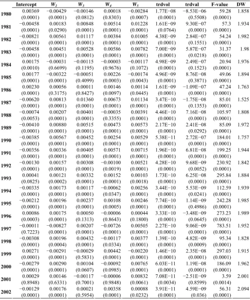
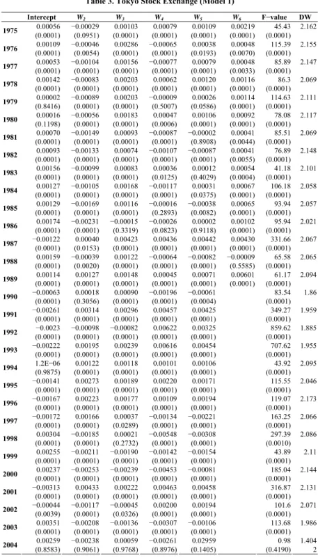
(8) 44. International Journal of Business and Economics Table 2. Hong Kong Stock Exchange (Model 2). 1980 1981 1982 1983 1984 1985 1986 1987 1988 1989 1990 1991 1992 1993 1994 1995 1996 1997 1998 1999 2000 2001 2002. Intercept 0.00369 (0.0001) −0.00458 (0.0001) −0.00821 (0.0001) −0.00458 (0.0001) 0.00175 (0.0010) 0.00177 (0.0001) 0.00230 (0.0001) −0.00620 (0.0001) −0.00074 (0.0053) −0.00410 (0.0001) −0.00385 (0.0001) −0.00356 (0.0001) −0.00130 (0.0001) 0.00041 (0.0825) −0.00335 (0.0001) −0.00212 (0.0001) 0.00086 (0.0003) −0.00011 (0.7223) −0.00308 (0.0001) 0.00271 (0.0001) −0.00279 (0.0001) 0.00029 (0.8948) −0.00129 (0.0001). W2 −0.00429 (0.0001) 0.00183 (0.0290) 0.00561 (0.0001) 0.00451 (0.0001) −0.00031 (0.6699) −0.00322 (0.0001) 0.00056 (0.3175) 0.00813 (0.0001) 0.00207 (0.0001) 0.00880 (0.0001) 0.00567 (0.0001) 0.00336 (0.0001) 0.00157 (0.0001) 0.00121 (0.0002) 0.00173 (0.0001) 0.00196 (0.0001) 0.00175 (0.0001) −0.00827 (0.0001) 0.00196 (0.0004) −0.00291 (0.0001) 0.00290 (0.0001) 0.00146 (0.6331) 0.00176 (0.0001). W3 −0.00146 (0.0812) 0.00848 (0.0001) 0.01117 (0.0001) 0.00528 (0.0001) −0.00115 (0.1195) −0.00051 (0.4099) 0.00011 (0.8427) 0.01360 (0.0001) 0.00401 (0.0001) 0.00515 (0.0001) 0.00452 (0.0001) 0.00405 (0.0001) 0.00308 (0.0001) 0.00332 (0.0001) 0.00117 (0.0001) 0.00237 (0.0001) 0.00050 (0.1313) 0.00207 (0.0001) 0.00432 (0.0001) −0.00029 (0.5831) 0.00104 (0.0607) −0.00117 (0.7001) 0.00021 (0.5954). W4 0.00018 (0.8303) 0.00514 (0.0001) 0.00384 (0.0001) 0.00586 (0.0001) −0.00003 (0.9676) 0.00226 (0.0003) 0.00146 (0.0097) 0.00673 (0.0001) −0.00035 (0.3355) 0.00473 (0.0001) 0.00254 (0.0001) 0.00571 (0.0001) −0.00100 (0.0019) 0.00152 (0.0001) −0.00062 (0.0347) 0.00108 (0.0005) −0.00006 (0.8643) −0.00726 (0.0001) −0.00117 (0.0334) 0.00442 (0.0001) −0.00092 (0.0985) −0.00006 (0.9848) 0.00358 (0.0001). W5 −0.00284 (0.0007) 0.01228 (0.0001) 0.01005 (0.0001) 0.00782 (0.0001) −0.00117 (0.1072) −0.00174 (0.0043) 0.00114 (0.0445) 0.01134 (0.0001) 0.00391 (0.0001) 0.00573 (0.0001) 0.00529 (0.0001) 0.00715 (0.0001) 0.00521 (0.0001) 0.00103 (0.0018) 0.00256 (0.0001) 0.00246 (0.0001) 0.00044 (0.1800) 0.00505 (0.0001) 0.00377 (0.0001) −0.00220 (0.0001) 0.00765 (0.0001) 0.00832 (0.0061) 0.00088 (0.0232). trdvol 1.77E−08 (0.0001) 1.61E−09 (0.0764) 4.38E−09 (0.0001) 7.00E−09 (0.0001) 4.98E−09 (0.0001) 4.96E−09 (0.0001) 1.61E−09 (0.0001) 3.47E−10 (0.0001) 4.46E−10 (0.0001) 2.17E−10 (0.0001) 5.38E−11 (0.0001) 1.96E−10 (0.0001) 4.28E−10 (0.0001) 1.73E−10 (0.0001) 3.44E−10 (0.0001) 7.74E−10 (0.0001) 3.33E−10 (0.0001) 2.27E−10 (0.0001) 1.39E−10 (0.0001) 1.46E−10 (0.0001) 6.03E−11 (0.0001) 7.08E−11 (0.0034) 3.91E−11 (0.0001). trdval F-value −8.53E−06 59.28 (0.5508) (0.0001) 9.30E−07 57.3 (0.0001) (0.0001) 2.84E−07 54.24 (0.1551) (0.0001) 5.87E−07 31.37 (0.0218) (0.0001) 2.49E−07 20.94 (0.1523) (0.0001) 8.76E−08 49.06 (0.3871) (0.0001) −1.09E−07 47.24 (0.0001) (0.0001) −1.75E−08 85.01 (0.1353) (0.0001) 7.16E−08 105.97 (0.0001) (0.0001) 2.41E−08 85.09 (0.0292) (0.0001) 2.72E−07 184.01 (0.0001) (0.0001) 6.81E−08 199.25 (0.0001) (0.0001) 9.68E−09 230.92 (0.0052) (0.0001) 6.25E−08 295.84 (0.0001) (0.0001) 5.53E−09 112.59 (0.0241) (0.0001) 1.14E−09 242.28 (0.4986) (0.0001) −3.48E−09 273.23 (0.0645) (0.0001) 9.06E−09 783.51 (0.0001) (0.0001) 4.82E−09 95.34 (0.0009) (0.0001) 2.35E−08 297.03 (0.0001) (0.0001) 1.19E−08 186.09 (0.0001) (0.0001) −2.51E−09 3.59 (0.8599) (0.0014) 4.59E−09 56.31 (0.036) (0.0001). DW 1.858 1.934 1.982 1.98 1.976 1.894 1.763 1.525 1.808 1.972 1.757 1.944 1.842 1.884 1.939 1.985 1.989 1.952 1.828 1.915 1.962 2.001 2.094. Table 3 contains the results of applying Model 1 to the data for years 1975 through 2004 for Tokyo Stock Exchange. Our results for Model 1 are similar to those for Hong Kong. Only nine of the coefficients for the daily dummy variable were not highly significant. Four of these occurred in 2004, suggesting exceptional circumstances that year. Due to the largeness of sample sizes, F-values were significant except for year 2004. Again the DW statistics were large enough (except for 2004) to support the validity of the significance tests for the coefficients. Thus, for the time period covered and sample firms studied, we again conclude that there are calendar effects and the weak form of EMH is in question..
(9) 45. Jeffrey E. Jarrett Table 3. Tokyo Stock Exchange (Model 1). 1975 1976 1977 1978 1979 1980 1981 1982 1983 1984 1985 1986 1987 1988 1989 1990 1991 1992 1993 1994 1995 1996 1997 1998 1999 2000 2001 2002 2003 2004. Intercept 0.00056 (0.0001) 0.00109 (0.0001) 0.00053 (0.0001) 0.00142 (0.0001) 0.00002 (0.8416) 0.00016 (0.1198) 0.00070 (0.0001) 0.00093 (0.0001) 0.00156 (0.0001) 0.00127 (0.0001) 0.00129 (0.0001) 0.00174 (0.0001) −0.00122 (0.0001) 0.00159 (0.0001) 0.00114 (0.0001) −0.00063 (0.0001) −0.00261 (0.0001) −0.0023 (0.0001) −0.00222 (0.0001) 1.2E−06 (0.9875) −0.00141 (0.0001) −0.00167 (0.0001) −0.00172 (0.0001) 0.00304 (0.0001) 0.00255 (0.0001) 0.00237 (0.0001) −0.00313 (0.0001) −0.00044 (0.0039) 0.00351 (0.0001) 0.00259 (0.8583). W2 −0.00029 (0.0951) −0.00046 (0.0054) −0.00104 (0.0001) −0.00083 (0.0001) −0.00089 (0.0001) −0.00056 (0.0001) −0.00149 (0.0001) −0.00133 (0.0001) −0.00099 (0.0001) −0.00105 (0.0001) −0.00169 (0.0001) −0.00231 (0.0001) 0.00040 (0.0153) −0.00039 (0.0020) 0.00127 (0.0001) 0.00018 (0.3056) 0.00314 (0.0001) −0.00098 (0.0001) 0.00195 (0.0001) 0.00122 (0.0001) 0.00273 (0.0001) 0.00223 (0.0001) 0.00166 (0.0001) −0.00185 (0.0001) −0.00211 (0.0001) −0.00253 (0.0001) 0.00433 (0.0001) −0.00117 (0.0001) −0.00208 (0.0001) −0.00238 (0.9061). W3 0.00103 (0.0001) 0.00286 (0.0001) 0.00156 (0.0001) 0.00203 (0.0001) 0.00203 (0.0001) 0.00183 (0.0001) 0.00093 (0.0001) 0.00074 (0.0001) 0.00083 (0.0001) 0.00168 (0.0001) 0.00116 (0.0001) −0.00015 (0.3319) 0.00423 (0.0001) 0.00122 (0.0001) 0.00148 (0.0001) 0.00090 (0.0001) 0.00296 (0.0001) −0.00082 (0.0001) 0.00239 (0.0001) 0.00118 (0.0001) 0.00189 (0.0001) 0.00177 (0.0001) 0.00037 (0.0289) 0.00021 (0.2732) −0.00190 (0.0001) −0.00239 (0.0001) 0.00222 (0.0001) −0.00045 (0.0326) −0.00136 (0.0001) 0.00059 (0.9768). W4 0.00079 (0.0001) −0.00065 (0.0001) −0.00077 (0.0001) 0.00062 (0.0001) −0.00009 (0.5007) 0.00047 (0.0006) −0.00087 (0.0001) −0.00107 (0.0001) 0.00036 (0.0125) −0.00117 (0.0001) −0.00016 (0.2893) −0.00026 (0.0823) 0.00436 (0.0001) −0.00064 (0.0001) 0.00045 (0.0001) −0.00196 (0.0001) 0.00457 (0.0001) 0.00622 (0.0001) 0.00616 (0.0001) 0.00101 (0.0001) 0.00220 (0.0001) 0.00109 (0.0001) −0.00134 (0.0001) −0.00548 (0.0001) −0.00142 (0.0001) −0.00453 (0.0001) 0.00463 (0.0001) 0.00200 (0.0001) −0.00307 (0.0001) −0.00261 (0.8976). W5 0.00109 (0.0001) 0.00038 (0.0193) 0.00079 (0.0001) 0.00120 (0.0001) 0.00026 (0.0586) 0.00106 (0.0001) −0.00002 (0.8908) −0.00087 (0.0001) 0.00012 (0.4029) 0.00031 (0.0375) −0.00038 (0.0082) 0.00002 (0.9118) 0.00442 (0.0001) −0.00082 (0.0001) 0.00071 (0.0001) −0.00061 (0.0004) 0.00425 (0.0001) 0.00325 (0.0001) 0.00454 (0.0001) 0.00106 (0.0001) 0.00171 (0.0001) 0.00194 (0.0001) −0.00221 (0.0001) −0.00308 (0.0001) −0.00154 (0.0001) −0.00081 (0.0001) 0.00458 (0.0001) 0.00194 (0.0001) −0.00106 (0.0001) 0.02959 (0.1405). W6 F−value 0.00219 45.43 (0.0001) (0.0001) 0.00048 115.39 (0.0070) (0.0001) 0.00048 85.89 (0.0033) (0.0001) 0.00116 86.3 (0.0001) (0.0001) 0.00114 114.63 (0.0001) (0.0001) 0.00092 78.08 (0.0001) (0.0001) 0.00041 85.51 (0.0044) (0.0001) 0.00041 76.89 (0.0055) (0.0001) 0.00054 41.18 (0.0004) (0.0001) 0.00067 106.18 (0.0001) (0.0001) 0.00065 93.94 (0.0001) (0.0001) 0.00102 95.94 (0.0001) (0.0001) 0.00430 331.66 (0.0001) (0.0001) −0.00009 65.58 (0.5585) (0.0001) 0.00601 61.17 (0.0001) (0.0001) 83.54 (0.0001) 349.27 (0.0001) 859.62 (0.0001) 707.62 (0.0001) 43.92 (0.0001) 115.55 (0.0001) 119.07 (0.0001) 163.25 (0.0001) 297.39 (0.0010) 43.89 (0.0001) 185.04 (0.0001) 316.87 (0.0001) 101.6 (0.0001) 113.68 (0.0001) 0.98 (0.4190). DW 2.162 2.155 2.147 2.069 2.111 2.117 2.069 2.148 2.101 2.058 2.057 2.021 2.067 2.065 2.094 1.86 1.959 1.885 1.955 2.095 2.046 2.173 2.066 2.086 2.11 2.144 2.131 2.071 1.986 1.404 2.
(10) 46. International Journal of Business and Economics Table 4. Tokyo Stock Exchange (Model 2). 1975 1976 1977 1978 1979 1980 1981 1982 1983 1984 1985 1986 1987 1988 1989 1990 1991 1992 1993 1994 1995 1996 1997 1998 1999 2000 2001 2002 2003 2004. Intercept −0.00023 (0.0702) 0.00032 (0.0064) −0.00011 (0.3136) 0.00050 (0.0001) −0.00042 (0.0001) −0.00045 (0.0001) 0.00037 (0.0001) 0.00056 (0.0001) 0.00093 (0.0001) 0.00052 (0.0001) 0.00072 (0.0001) 0.00133 (0.0001) −0.00139 (0.0001) 0.00140 (0.0001) 0.00065 (0.0001) −0.00124 (0.0001) −0.00323 (0.0001) −0.00280 (0.0001) −0.00289 (0.0001) −0.00052 (0.0001) −0.00198 (0.0001) −0.00226 (0.0001) −0.00183 (0.0001) 0.00271 (0.0001) 0.00173 (0.0001) 0.00157 (0.0001) −0.00345 (0.0001) −0.00068 (0.0001) 0.00300 (0.0001) −0.00175 (0.9040). W2 −0.00037 (0.0319) −0.00053 (0.0011) −0.00113 (0.0001) −0.00095 (0.0001) −0.00093 (0.0001) −0.00063 (0.0001) −0.00155 (0.0001) −0.00138 (0.0001) −0.00109 (0.0001) −0.00112 (0.0001) −0.00177 (0.0001) −0.00237 (0.0001) 0.00036 (0.0285) −0.00044 (0.0005) 0.00113 (0.0001) 0.00010 (0.5701) 0.00301 (0.0001) −0.00103 (0.0001) 0.00186 (0.0001) 0.00116 (0.0001) 0.00270 (0.0001) 0.00213 (0.0001) 0.00164 (0.0001) −0.00189 (0.0001) −0.00218 (0.0001) −0.00254 (0.0001) 0.00431 (0.0001) −0.00118 (0.0001) −0.00212 (0.0001) −0.00250 (0.9014). W3 0.00090 (0.0001) 0.00266 (0.0001) 0.00139 (0.0001) 0.00178 (0.0001) 0.00191 (0.0001) 0.00168 (0.0001) 0.00082 (0.0001) 0.00063 (0.0001) 0.00070 (0.0001) 0.00143 (0.0001) 0.00097 (0.0001) −0.00029 (0.0554) 0.00416 (0.0001) 0.00112 (0.0001) 0.00130 (0.0001) 0.00060 (0.0001) 0.00282 (0.0001) −0.00094 (0.0001) 0.00225 (0.0001) 0.00106 (0.0001) 0.00180 (0.0001) 0.00161 (0.0001) 0.00034 (0.0454) 0.00015 (0.4291) −0.00201 (0.0001) −0.00242 (0.0001) 0.00218 (0.0001) −0.00046 (0.0278) −0.00141 (0.0001) 0.00031 (0.9878). W4 0.00060 (0.0005) −0.00077 (0.0001) −0.00092 (0.0001) 0.00046 (0.0024) −0.00018 (0.1780) 0.00035 (0.0095) −0.00094 (0.0001) −0.00117 (0.0001) 0.00020 (0.1531) −0.00133 (0.0001) −0.00032 (0.0298) −0.00039 (0.0088) 0.00429 (0.0001) −0.00072 (0.0001) 0.00031 (0.0061) −0.00210 (0.0001) 0.00443 (0.0001) 0.00604 (0.0001) 0.00601 (0.0001) 0.00090 (0.0001) 0.00210 (0.0001) 0.00094 (0.0001) −0.00137 (0.0001) −0.00554 (0.0001) −0.00157 (0.0001) −0.00457 (0.0001) 0.00458 (0.0001) 0.00198 (0.0001) −0.00311 (0.0001) −0.00288 (0.8871). W5 W6 trdvol trdval F−value DW 0.00085 0.00227 2.68E−09 6.2E−06 538.13 2.169 (0.0001) (0.0001) (0.0001) (0.0001) (0.0001) 0.00023 0.00058 1.00E−09 7.8E−06 738.91 2.163 (0.1616) (0.0012) (0.0001) (0.0001) (0.0001) 0.00059 0.00055 1.81E−09 4.4E−06 686.5 2.155 (0.0001) (0.0008) (0.0001) (0.0001) (0.0001) 0.00095 0.00125 1.29E−10 1.0 E−06 1019.18 2.078 (0.0001) (0.0001) (0.0195) (0.0001) (0.0001) 0.00015 0.00118 1.02E−09 1.7 E−06 689.32 2.121 (0.2513) (0.0001) (0.0001) (0.0001) (0.0001) 0.00092 0.00100 1.00E−10 5.3E−06 915.99 2.13 (0.0001) (0.0001) (0.0041) (0.0001) (0.0001) −0.00011 0.00046 1.21E−11 2.2E−06 488.83 2.076 (0.3936) (0.0013) (0.6466) (0.0001) (0.0001) −0.0010 0.00043 1.05E−09 1.3E−06 491.83 2.156 (0.0001) (0.0034) (0.0001) (0.0001) (0.0001) −0.00005 0.00065 1.01E−09 2.4E−06 787.05 2.109 (0.7016) (0.0001) (0.0001) (0.0001) (0.0001) 908.09 2.068 0.00009 0.00081 1.41E−09 2.1E−06 (0.5561) (0.0001) (0.0001) (0.0001) (0.0001) −0.00053 0.00079 7.83E−10 1.7E−06 747.59 2.066 (0.0003) (0.0001) (0.0001) (0.0001) (0.0001) −0.00013 0.00110 1.77E−10 8.68E−07 599.76 2.026 (0.3941) (0.0001) (0.0001) (0.0001) (0.0001) 0.00435 0.00432 3.09E−10 1.76E−09 423.94 2.07 (0.0001) (0.0001) (0.0001) (0.003) (0.0001) −0.00090 −0.00005 3.10E−10 2.02E−09 337.82 2.069 (0.0001) (0.7275) (0.0001) (0.0252) (0.0001) 0.00058 0.00581 9.73E−10 2.99E−09 810.66 2.102 (0.0001) (0.0001) (0.0001) (0.0177) (0.0001) −0.00078 2.19E−10 1.2E−06 442.18 1.862 (0.0001) (0.0011) (0.0001) (0.0001) 0.00405 8.96E−10 1.5E−06 815.57 1.964 (0.0001) (0.0001) (0.0001) (0.0001) 0.00302 1.99E−09 1.2E−06 797.52 1.89 (0.0001) (0.0001) (0.0001) (0.0001) 0.00425 2.73E−09 6.01E−07 1051.65 1.96 (0.0001) (0.0001) (0.0001) (0.0001) 0.00093 2.35E−09 3.35E−07 446.08 2.098 (0.0001) (0.0001) (0.0001) (0.0001) 0.00154 1.70E−09 0.00000108 496.59 2.053 (0.0001) (0.0001) (0.0001) (0.0001) 0.00169 2.39E−09 4.85E−07 618.85 2.18 (0.0001) (0.0001) (0.0001) (0.0001) −0.00224 −9.80E−10 0.00000144 254.55 2.064 (0.0001) (0.0001) (0.0001) (0.0001) −0.00316 1.46E−09 −5.54E−08 281.38 2.088 (0.0001) (0.0001) (0.5189) (0.0001) −0.00180 2.23E−09 4.59E−07 631.8 2.117 (0.0001) (0.0001) (0.0001) (0.0001) −0.00094 2.46E−09 −4.78E−08 579.11 2.148 (0.0001) (0.0001) (0.0146) (0.0001) 0.00450 7.34E−10 1.72E−07 326.46 2.13 (0.0001) (0.0001) (0.0001) (0.0001) 0.00190 5.08E−10 1.40E−07 102.31 2.071 (0.0001) (0.0001) (0.0027) (0.0001) −0.00112 7.67E−10 2.35E−07 550.49 1.986 (0.0001) (0.0001) (0.0001) (0.0001) 0.02903 −7.18E−10 8.6E−06 2.97 2 (0.1482) (0.6981) (0.0003) (0.0068).
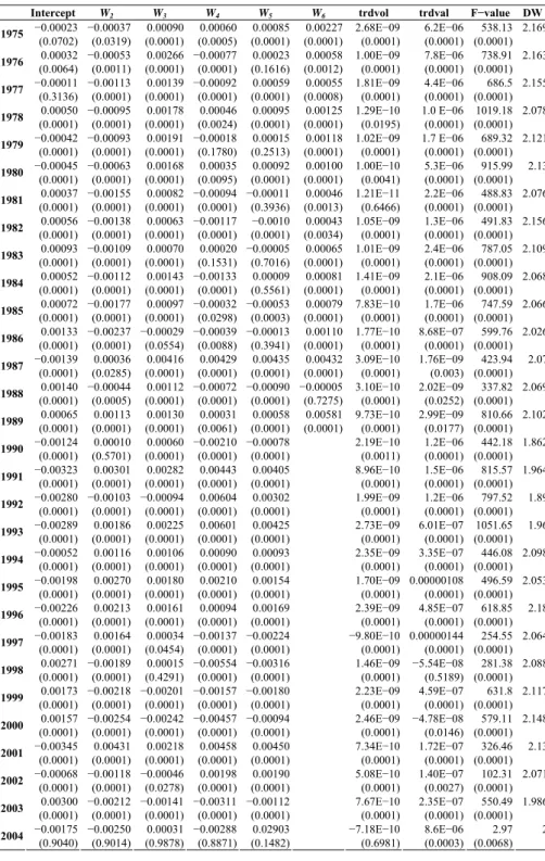
(11) Jeffrey E. Jarrett. 47. Model 2 regressions for the Tokyo Stock Exchange (Table 4) produced results similar to those in Table 3. With the exception of 2004, the results indicate the daily influences on the returns to Japanese securities listed on the Tokyo Stock Exchange were very similar to the results in Table 3. The inclusion of the trdvol and trdval variables did not alter the general conclusion of the earlier findings for Hong Kong in Tables 1 and 2. We note that of the 15 years with Saturday trading days only year 1988 did not produce a highly significant regression coefficient. Hence, Saturday, for the most part, evidenced different trading patterns from the other days of the week for these years. The four tables containing approximately 80 multiple regressions for very large samples suggest that trading on these two large exchanges differed by day of the week. Also, the DW statistics failed to reject the hypothesis that serial correlation is present. This supports the validity of the numerous significance tests. We should note that some researchers agree that stock return data have heavy tails and tend not to be normally distributed, so the OLS results may be suspect. In particular, outliers may result in inconsistent estimators. Some argue that autoregressive conditional heteroscedastic methods are needed to correct for correlated data and non-constant variance. Incorrect standard errors lead to incorrect significance tests. As in previous studies, we considered analyzing a portion of the data using quantile regression along the lines of Cho et al. (2007). Based on their results, we expect this analysis would be similar to our OLS results and the new analysis is unnecessary. Cho et al. (2007) contain in their studies sufficient evidence to make our results valid. Note Tables 1-4 summarize our entire analysis. Our purpose was to analyze the results for individual firms and not for stock indexes. We could have focused on a few firms over a long period or studied a large number of sampled firms for a short period. Others have done this. The achievement of this study is not a statistical exercise but an analytical study to explain the economic behavior of markets. The Hong Kong and Tokyo stock exchanges are established markets with established regulations and a large and world-wide constituency. We established in this study the relationship between economic explanations of financial events and analytical results concerning a large sample of firms over a lengthy time period on two well-established Asian financial markets. A study of this magnitude has not been published in this journal with these data. 5. Conclusions We document in this study that daily closing prices for a large number of firms listed on two of the largest Asian stock exchanges contain properties that one can measure, model, and use for prediction. With enough time, patience, and understanding of the underlying processes that give rise to stock return series, forecasters can properly model these data. The results permit management scientists and financial forecasters to recognize that return series of listed securities are not random and do have daily affects..
(12) 48. International Journal of Business and Economics. In this study, we indicate the presence of time series components in stock returns for randomly selected sets of firms. The results corroborate results of a number of earlier but less exhaustive studies. Calendar and daily effects exist in the financial time series stock returns studied. When these properties in security returns exist, one may identify and forecast patterns in financial data, and, in turn, investors may benefit from this information. Furthermore, the results indicate that the weak form of the EMH is in question when one must make decisions concerned with investing in stock market securities. Daily variation is not entirely random and possibilities exist to predict daily patterns with some degree of accuracy. We suggest, for purposes of prediction, that forecasters model systematic time series components of security returns. In addition, one cannot understate the importance of stock returns and portfolio risk. These factors coupled with recognition of systematic time series components (daily variation in this study) in stock prices can improve price forecasting of individual securities and contribute to the literature on capital market efficiency. One last question concerns the out-of sample trading profit opportunities. Finding in-sample profit opportunities can be thought of as a “data-mining” result, that is, if you fit many models, a few will randomly have high coefficients of determination and/or statistically significant model coefficients. We suggest using parsimonious models; profit opportunities should be greater than transaction costs that may include bid-ask spreads and commissions. If so, we can find profitable trading opportunities in rapidly growing Asian markets. When the opportunity arises to examine data for Shanghai and other emerging Asian exchanges, we expect additional studies of those large and growing markets. We are only limited by our ability to collect sufficient and reliable data. References Alesii, G., (2006), “Fundamentals Efficiency of the Italian Stock Market: Some Long Run Evidence,” International Journal of Business and Economics, 5(3), 245-264. Balvers, R. J., T. F. Cosimano, and B. McDonald, (1990), “Predicting Stock Returns in an Efficient Market,” Journal of Finance, 45, 1109-1128. Black, A. and P. Fraser, (1995), “UK Stock Returns: Predictability and Business Conditions,” The Manchester School of Economic & Social Studies, 63, 85102. Breen, W., L. R. Glosten, and R. Jagannathan, (1990), “Economic Significance of Predictable Variations in Stock Index Returns,” Journal of Finance, 44(5), 1177-1189. Campbell, J. Y., (1987), “Stock Returns and the Term Structure,” Journal of Financial Economics, 18(2), 373-399..
(13) Jeffrey E. Jarrett. 49. Caporale, G. M. and L. A. Gil-Alana, (2002), “Fractional Integration and Mean Reversion in Stock Prices,” Quarterly Review of Economics and Finance, 42(3), 599-609. Clare, A. D., S. H. Thomas, and M. R. Wickens, (1994), “Is the Gilt-Equity Yield Ratio Useful for Predicting UK Stock Returns?” Economic Journal, 104, 303-315. Clare, A. D., Z. Psaradakis, and S. H. Thomas, (1995), “An Analysis of Seasonality in the UK Equity Market,” Economic Journal, 105, 398-409. Cho, Y. H., O. Linton, and Y. J. Whang, (2007), “Are There Monday Effects in Stock Returns: A Stochastic Dominance Approach,” Journal of Empirical Finance, 14(5), 736-755. Coutts, J. A. and P. A. Hayes, (1999) “The Weekend Effect, the Stock Exchange Account and the Financial Times Industrial Ordinary Shares Index: 19871994,” Applied Financial Economics, 9, 67-71. Dickey, D. A. and W. A. Fuller, (1979), “Distribution of the Estimators for Autoregressive Time Series with a Unit Root,” Journal of the American Statistical Association, 74, 427-431. Fama, E. F., (1965), “The Behavior of Stock-Market Prices,” Journal of Business, 38, 34-105. Fama, E. F., (1970), “Efficient Capital Markets: A Review of Theory and Empirical Work,” Journal of Finance, 25, 383-417. Fama, E. F. and K. R. French, (1989), “Business Conditions and Expected Returns on Stocks and Bonds,” Journal of Financial Economics, 25, 23-49. Francis, J. C., (1993), Management of Investments, New York: McGraw-Hill. Goh, K. and K. Kok, (2006), “Beating the Random Walk: Intraday Seasonality and Volatility in a Developing Stock Market,” International Journal of Business and Economics, 5(1), 29-40. Granger, C. W. J., (1992), “Forecasting Stock Market Prices: Lessons for Forecasters,” International Journal of Forecasting, 8, 3-13. Hamori, S. and A. Tokihisa, (2002), “Some International Evidence on the Seasonality of Stock Prices,” International Journal of Business and Economics, 1(1), 79-86. Jarrett, J. and E. Kyper, (2005a), “Daily Variation, Capital Market Efficiency and Predicting Stock Market Returns,” Management Research News, 28(8), 34-47. Jarrett, J. and E. Kyper, (2005b), “Evidence on the Seasonality of Stock Market Prices of Firms Traded on Organized Markets,” Applied Economics Letters, 12, 537-543. Jarrett, J. and E. Kyper, (2006), “Capital Market Efficiency and the Predictability of Daily Returns,” Applied Economics, 38, 631-636. Kato, K., (1990a), “Weekly Patterns in Japanese Stock Returns,” Management Science, 36, 1031-1043. Kato, K., (1990b), “Being a Winner in the Tokyo Stock Market,” Journal of Portfolio Management, 16, 52-56..
(14) 50. International Journal of Business and Economics. Kubota, K. and H. Takahara, (2003), “Financial Sector Risk and the Stock Returns: Evidence from Tokyo Stock Exchange Firms,” Asia-Pacific Financial Markets, 10(1), 1-28. Lo, A. W. and A. C. MacKinley, (1988), “Stock Market Prices Do Not Follow Random Walks: Evidence from a Simple Specification Test,” Review of Financial Studies, 1, 41-66. Lo, A. W. and A. C. MacKinley, (1990), “When are Contrarian Profits Due to Stock Market Overreaction?” Review of Financial Studies, 3, 175-205. Lucas, Jr. R. E., (1978), “Asset Prices in an Exchange Economy,” Econometrica, 46(6), 1429-1445. MacKinnon, J. G., (1991), “Critical Values for Cointegration Tests,” in Long-Run Economic Relationships: Readings in Cointegration, R. F. Engle and C. W. J. Granger eds., Oxford University Press, Chapter 13. Moorkejee, R. and Q. Yu, (1999), “Seasonality in Returns on the Chinese Stock Markets: The Case of Shanghai and Shenzhen,” Global Finance Journal, 10, 93-105. Pesaran, M. H. and A. Timmermann, (1995), “Predictability of Stock Returns: Robustness and Economic Significance,” Journal of Finance, 50(4), 12011228. Pesaran, M. H. and A. Timmermann, (2000), “A Recursive Modelling Approach to Predicting UK Stock Returns,” The Economic Journal, 110, 159-191. Pettengill, G., (2003), “A Survey of the Monday Effect Literature,” Quarterly Journal of Business and Economics, 42(3/4), 3-27. Poterba, J. M. and L. H. Summers, (1988), “Mean Reversion in Stock Prices: Evidence and Implications,” Journal of Financial Economics, 22, 27-59. Ray, B., S. Chen, and J. Jarrett, (1997), “Identifying Permanent and Temporary Components in Daily and Monthly Japanese Stock Prices,” Financial Engineering and the Japanese Markets, 4(3), 233-256. Rothlein, C. J. and J. Jarrett, (2002), “Seasonality in Prices of Japanese Securities,” International Journal of Business & Economics, 1, 21-31. Shum, W. C. and G. Y. N. Tang, (2005), “Common Risk Factors in Returns in Asian Emerging Stock Markets,” International Business Review, 14(6), 695717. Skidelsky, L. R., (1992), John Maynard Keynes, Vol. 2, Macmillan Publishers. Steeley, J. M., (2001), “A Note on Information Seasonality and the Disappearance of the Weekend Effect in the UK Stock Market,” Journal of Banking and Finance, 25, 1941-1956. Tian, G. G., G. H. Wan, and M. Guo, (2002), “Market Efficiency and the Returns to Simple Technical Trading Rules: New Evidence from U.S. Equity Market and Chinese Equity Markets,” Financial Engineering and the Japanese Markets, 9(3-4), 241-258. Wong, M. C. S., Y.-L. Cheung, and L. Wu, (2000), “Insider Trading in the Hong Kong Stock Market,” Financial Engineering and the Japanese Markets, 7(3), 275-288..
(15) Jeffrey E. Jarrett. 51. Ho, Y.-K. R., (1998), “The Hong Kong Securities Markets: Review and Prospects,” Financial Engineering and the Japanese Markets, 5(1), 29-44. Yonezawa, Y. and K. Miyake, (1998), “The Structure of the Japanese Stock Market,” Financial Engineering and the Japanese Markets, 5(1), 1-28..
(16)
數據

相關文件
5.1.1 This chapter presents the views of businesses collected from the business survey, 12 including on the number of staff currently recruited or relocated or planned to recruit
In the past 5 years, the Government has successfully taken forward a number of significant co-operation projects, including the launch of Shanghai- Hong Kong Stock Connect
The above information is for discussion and reference only and should not be treated as investment
Warrants are an instrument which gives investors the right – but not the obligation – to buy or sell the underlying assets at a pre- set price on or before a specified date.
This thesis applied Q-learning algorithm of reinforcement learning to improve a simple intra-day trading system of Taiwan stock index future. We simulate the performance
The one we saw earlier (p. 305) models the stock price minus the present value of the anticipated dividends as following geometric Brownian motion.. One can also model the stock
The fuzzy model, adjustable with time, is first used to consider influence factors with different features such as macroeconomic factors, stock and futures technical indicators..
That is, when these records produced association rule: “Stock A drop Î Stock B drop”, the rule shows that when stock A drops, stock B drops with high probability on the same day..
