國 立 交 通 大 學
電子工程學系 電子研究所碩士班
碩 士 論 文
MPEG-4 物件視訊解碼器在 PACDSP 平台上之
軟體實現
Software Implementation of MPEG-4 Object-Based Video
Decoder on PACDSP Platform
研 究 生 : 許介遠
指導教授 : 林大衛 博士
MPEG-4 物件視訊解碼器在 PACDSP 平台上之軟體實現
Software Implementation of MPEG-4 Object-Based Video
Decoder on PACDSP Platform
研 究 生 : 許介遠
Student: Chieh Yuan Hsu
指導教授 : 林大衛 博士
Advisor: Dr. David W. Lin
國 立 交 通 大 學
電子工程學系 電子研究所碩士班
碩士論文
A Thesis
Submitted to Department of Electronics Engineering & Institute of Electronics College of Electrical and Computer Engineering
National Chiao Tung University in Partial Fulfillment of the Requirements
for the Degree of Master of Science
in
Electronics Engineering June 2007
Hsinchu, Taiwan, Republic of China
MPEG-4 物件視訊解碼器在 PACDSP 平台上
之軟體實現
研究生: 許介遠 指導教授:林大衛 博士
國立交通大學電子工程學系 電子研究所碩士班
摘要
MPEG-4 為一廣泛應用之多媒體訊號壓縮標準。本篇論文介紹在 PACDSP 平台上 MPEG-4 物件視訊解碼器之實現,本平台由一超長指令數位訊號處理器 與一 ARM920T 處理器所組成。為了最佳化程式流程,我們完成了許多的靜態分 析,並且利用超長指令處理器架構上之特性來達到即時解碼。我們也完成了雙核 心的實現以提高整體的效能。 在我們的實作當中,我們使用了 MPEG-4 參考軟體,MoMuSys,當作驗證 的比較對象。首先,我們分析了 MPEG-4 基於物件解碼器之運算複雜度並藉此 找到有效率的實現方法。為了能減少運算量以及在 PACDSP 上實現,我們將離 散餘弦反轉換(IDCT)轉為整數點運算(fixed point),並且討論其效能及精確度。 最後,我們的實現之精確度能夠符合 IEEE 1180-1190 標準之規範。同時,我們 所使用之演算法在效能上也具有與其他實現競爭的能力。接著,我們討論了在雙 核心平台上的實現方法以提高效能。為了加速執行時間,我們利用了 PACDSP的特性,將規律之運算分佈於兩組以增加處理器之效能。我們也使用單指令多資 料(SIMD)指令以及一般指令層級平行化來減少處理器之延遲。在演算法上, 我們根據離散餘弦轉換(DCT)之特性來跳過多餘的運算。在所有的最佳化之後, 我們在最差情況下,對於一個工作在 200MHz 的真實 PACDSP 晶片而言,能夠 達到每秒 46 張的解碼,滿足每秒三十張即時解碼的要求。而整個程式的大小為 30 Kbytes,也小於 PACDSP 的程式快取記憶體大小 32 Kbytes。最後我們在 PSDK 平台上展示了雙核心的實現結果。
在本篇論文當中,我們首先介紹了 MPEG-4 標準以及 PADSP 平台之概述。 接著討論靜態分析、雙核心實現之設計、實作策略、最佳化方法、以及最後實現 之結果。
Software Implementation of MPEG-4 Object-Based
Video Decoder on PACDSP Platform
Student: Chieh-Yuan Hsu
Advisor: Dr. David W. Lin
Department of Electronics Engineering
Institute of Electronics
National Chiao Tung University
Abstract
MPEG-4 is a widely-applied multimedia coding standard. This thesis presents an implementation of the MPEG-4 object-based video decoder on the PACDSP platform, which consists of a VLIW digital signal processor (DSP) and an ARM920T processor. We complete many analyses to optimize the program flow and utilize the advantage of VLIW processor to achieve real-time decoding. Finally, a dual-core demonstration is completed and verified.
In our implementation, the MPEG-4 reference software, MoMuSys, is used as a model to verily our implementation. First, we analyze the computational complexity of the MPEG-4 object-based video decoder, and find efficient algorithms for the implementation. In order to reduce the complexity and to realize on PACDSP, we implement the fixed point inverse discrete cosine transform (IDCT), and then discuss the efficiency and accuracy. At last, our implementation can pass the accuracy test of
IEEE 1180-1190 standard and the performance of our algorithm is also competitive to other implementations. Then, we discuss the design of dual-core implementation to improve the performance. In order to speed up the execution time, we distribute the regular computations to both clusters to increase the efficiency of the processor. Single-instruction-multiple-data (SIMD) instructions and general instruction level parallelism also utilized to reduce the processor stalls. For algorithmic optimization, we skip unnecessary computations according to the nature of discrete cosine transform (DCT). After all the optimizations, in the worst case, our implementation of decoder decodes 46 frame-per-second, which can achieve real-time decoding, 30 frame-per-second, for a real PACDSP chip running over 200 MHz. The code size is 30 Kbytes, which is smaller than the 32 Kbytes instruction cache on PACDSP. Finally, we demonstrate a dual-core implementation on the PAC System Developer’s Kit (PSDK).
In this thesis, we first introduce the MPEG-4 standard and give an overview of the PACDSP platform. Then the static analysis, dual-core design, implementation strategies, the optimization methods, and the results of our implementation are discussed.
誌謝
本篇論文的完成,誠摯地感謝我的指導老師 林大衛 博士,從踏入交通大學 電子所開始,多虧老師的循循善誘,不但給予我在課業、研究上的幫助,使我學 到了分析問題及解決問題的能力。同時老師樂觀的生活態度也影響了我,讓我更 有勇氣面對各種困難。在此,僅向老師及老師的家人致上最高的感謝之意。 感謝在電子研究所 CommLab 這個大家族的日子裡,實驗室所提供完善的研究 資源。承蒙崑健、家揚、俊榮、朝雄、鴻志、亦善、榮煌等學長的提攜與照顧。 而實驗室的同伴,政達、志岡、育群、柏昇、耀鈞、凱庭、錫祺、浩廷、育成、 順成等,在課業上的砥礪與生活上的幫助也讓我在忙碌的研究所生涯中仍舊擁有 快樂的心情。 最後,感謝我的家人,溫暖的家一直是我求學生涯中最強而有力的後盾,感 謝你們的努力讓我能夠無後顧之憂地汲取知識,繼續升學。僅將本論文獻給我敬 愛的父母,許回福先生、廖淑香女士。 許介遠 民國九十六年六月于新竹
Contents
1 Introduction 1
2 Overview of the MPEG-4 Video Standard 3
2.1 Structure of MPEG-4 Video Data . . . 3
2.2 MPEG-4 Video Texture Coding . . . 6
2.2.1 Shape Coding . . . 6
2.2.2 Motion Coder . . . 9
2.2.3 Texture Coder . . . 15
2.2.4 Other Video Coding Tools [7] . . . 18
2.3 Profiles and Levels [5] . . . 20
3 Overview of PACDSP 23 3.1 Introduction . . . 23
3.2 Program Sequence Control Unit . . . 24
3.2.1 Branch Instructions . . . 25
3.2.2 Loop . . . 26
3.2.3 Customized Function Units . . . 27
3.2.4 Exception Handling . . . 27
3.2.5 Interrupt Handling . . . 27
3.3 VLIW Datapath . . . 28
3.3.1 Arithmetic Unit (AU) . . . 28
3.3.2 Load/Store Unit (L/S) . . . 28
3.3.4 Data/Address/Accumulator Registers . . . 30
3.3.5 Status and Control Registers . . . 31
3.3.6 Addressing Modes . . . 32
3.3.7 Data Exchange . . . 34
3.3.8 Constant Register File . . . 36
3.4 Scalar Unit . . . 37
3.4.1 Scalar Unit . . . 37
3.4.2 Control Registers . . . 37
3.4.3 General Purpose Scalar Register File . . . 38
3.5 Conditional Execution Control . . . 38
3.6 ISA and Pipeline Stages . . . 40
3.7 DSP Running Modes . . . 40
3.8 Instruction Packet . . . 41
3.9 Development Tools and Implementation Approach . . . 42
3.9.1 Development Tools . . . 42
3.9.2 Implementation approach . . . 43
3.10 Overview of the PSDK 2.0 Platform . . . 45
3.11 Overview of PACDSP v3.0 . . . 45
3.11.1 Architecture Overview . . . 46
3.11.2 Program Control Sequence Unit (PSCU) . . . 47
3.11.3 VLIW Datapath . . . 48
3.11.4 Pipeline Stages . . . 49
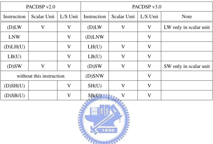
3.11.5 Instruction Set Comparison . . . 49
4 Complexity Analysis of MPEG-4 Object-Based Video Decoder and Dual-Core Implementation Design 51 4.1 Profiles of the MPEG-4 Object-Based Video Decoder . . . 52
4.2 Fixed-Point IDCT . . . 55
4.2.1 Efficiency of IDCT . . . 56
4.2.3 Profile on PC with Fixed-Point IDCT . . . 58
4.3 Implementation of Decoder on Dual-Core PSDK . . . 59
4.4 Optimization of Implementation on ARM . . . 61
5 Optimization of Implementation on PACDSP 64 5.1 Implementation Strategies on PACDSP . . . 65
5.1.1 Efficient Context-Based Arithmetic Coding . . . 65
5.1.2 Efficient Variable Length Decoding (VLD) . . . 69
5.1.3 Efficient AC/DC Reconstruction . . . 74
5.1.4 Optimization of IDCT on PACDSP . . . 79
5.2 Architectural Optimization . . . 79
5.2.1 General Optimization Techniques . . . 80
5.2.2 Advantages of PACDSP . . . 83
5.2.3 Experiment Result of Architectural Optimization . . . 83
5.3 Algorithmic Optimization . . . 84
5.3.1 Efficient Inverse Scan . . . 84
5.3.2 Efficient IQ and IDCT . . . 87
5.3.3 Experiment Result of Algorithmic Optimization . . . 88
5.4 Conclusion . . . 89
6 Overall Performance of the Implementation 93 6.1 Performance Analysis . . . 93
6.2 Effect of Different Quantization Steps (QP) . . . 98
7 Conclusion and Future Work 103 7.1 Conclusion . . . 103
List of Figures
2.1 Segmentation of a frame into VOPs (from [7]). . . 4
2.2 Structure of coded video data (from [8]). . . 5
2.3 Types of VOP. . . 5
2.4 Positions of luminance and chrominance samples in 4:2:0 data (from [9]). 7 2.5 Simplified structure of the video decoder (from [5]). . . 8
2.6 Pixel templates used for (a) INTRA and (b) INTER context calculation of BAB. The current pixel to be coded is marked with “?” (from [5]). . . 10
2.7 Simplified padding process (from [5]). . . 11
2.8 Priority of boundary MBs surrounding an exterior MB(from [5]). . . 12
2.9 Motion vector prediction (from [9]). . . 13
2.10 Quantizers in H.263. (a) For intra DC coefficient only. (b) For inter DC and all AC coefficients. . . 17
2.11 Prediction of DC coefficients of blocks in an intra MB (from [7]). . . 17
2.12 Prediction of AC coefficients of blocks in an intra MB (from [7]). . . 19
2.13 Scans for8 × 8 blocks (from [5]). . . 19
3.1 Architecture of the PACDSP (from [1]). . . 25
3.2 Illustration of multiplication instructions with different precisions (from [1]). . . 29
3.3 Different load/store instructions (from [1]). . . 30
3.4 Ping-pong register file in one cluster (from [1]). . . 31
3.5 Available registers in one cluster (from [1]). . . 32
3.7 Data broadcast among clusters (from [1]). . . 35
3.8 The Constant Register File of one cluster (from [1]). . . 38
3.9 PACDSP instruction set architecture (from [1]). . . 41
3.10 Pipeline stages of the PACDSP (from [1]). . . 41
3.11 Transitions between DSP running modes (from [1]). . . 44
3.12 Simplified syntax of instruction packet (from [1]). . . 45
3.13 PAC System Developer’s Kit (PSDK) 2.0. . . 46
3.14 Memory map of the dualcore demonstration . . . 47
3.15 Architecture of PACDSP v3.0 (from [2]). . . 48
3.16 Pipeline stages of the PACDSP v3.0 (from [4]). . . 49
4.1 Block diagram of MPEG-4 object-based video decoder [5]. . . 52
4.2 First frame of each test sequence (a) stefan. (b) foreman. (c) akiyo. . . 53
4.3 The IDCT algorithm used in MoMuSys [10]. . . 58
4.4 The even-odd decomposition IDCT algorithm [12]. . . 59
4.5 An outline of P frame decoding procedure. . . 61
4.6 The dual-core P-frame decoding. . . 62
5.1 Flow of software development on PACDSP. . . 65
5.2 Pixel templates used for (a) INTRA and (b) INTER context calculation of BAB (from [5]). . . 67
5.3 Intra context calculation. . . 67
5.4 Fast intra context calculation. . . 68
5.5 Example assembly code for fast inter context calculation. . . 68
5.6 Calculation distribution of two clusters on PACDSP. . . 69
5.7 Example assembly code for getting reference BAB on PACDSP. . . 69
5.8 Example of one table mapping with magnitude-offset on PACDSP. . . 71
5.9 Example of bit-by-bit matching on PACDSP. . . 71
5.10 Example of multiple-pass matching on PACDSP. . . 72
5.11 Example of optimized multiple-pass matching on PACDSP. . . 73
5.13 DC/AC prediction in MPEG-4 video decoder. . . 76
5.14 (a) Total blocks in one MB. (b) Pixels store for DC/AC prediction of one block. . . 76
5.15 Memory usage design of DC/AC prediction for two successive MBs. . . . 77
5.16 Program flow of DC/AC prediction in MoMuSys. . . 78
5.17 Example C code of vector addition. . . 80
5.18 Example of static rescheduling technique. . . 82
5.19 Example of loop unrolling technique. . . 82
5.20 Example of software pipelining technique. . . 83
5.21 Program flow of texture decoding in MPEG-4 object-based video decoder. 85 5.22 Scan orders for8 × 8 blocks [5]. . . 86
5.23 DC spreading from decoded coefficient to output block. . . 87
5.24 Assembly code of DC spreading. . . 88
5.25 Program flow of texture decoding in MPEG-4 object-based video decoder after optimization. . . 91
5.26 Improvement in execution time of architectural and algorithmic optimiza-tions for I-frames on PACDSP. . . 92
5.27 Improvement in execution time of architectural and algorithmic optimiza-tions for P-frames on PACDSP. . . 92
List of Tables
2.1 List of BAB Types (from [5]) . . . 9
2.2 Weighting ValuesH0(i, j), H1(i, j), and H2(i, j) . . . 15
2.3 Default Quantization Matrix (Q) [5] . . . . 18
2.4 Nonlinear Scaler for DC Coefficients (from [5]) . . . 18
2.5 Profiles and Tools (from [5]) . . . 22
3.1 Details of Control Register Files (from [1]) . . . 39
3.2 Memory-Mapped Control Registers (from [1]) . . . 40
3.3 Pipeline Stages and Their Descriptions (from [1]) . . . 42
3.4 Running Modes of the PACDSP (from [1]) . . . 43
3.5 Instruction Types in Each Instruction Slot (from [1]) . . . 44
3.6 Modification of Load/Store Instructions from PACDSP v2.0 to PACDSP v3.0 . . . 50
3.7 Comparison Instructions Supported in PACDSP v2.0 and PACDSP v3.0 . 50 4.1 VOP Size of Each Test Sequence . . . 53
4.2 Profile of Object-Based MPEG-4 Decoding of QCIF Sequence on VTune 54 4.3 Comparison of Computational Complexity for 8-point IDCT . . . 56
4.4 Test of Compliance for Modified IEEE Std. 1180-1190 in MPEG-4 . . . . 60
4.5 Execution Time Comparison of IDCT . . . 60
4.6 Execution Time Analysis Between ARM and PACDSP . . . 63
4.7 Analysis of Necessary Interpolation Using MoMuSys Encoder . . . 63
4.8 Execution Time of Motion Compensation after Eliminating Unnecessary Interpolations on ARM . . . 63
5.1 Execution Time Comparison of Context Calculation for One BAB on
PACDSP . . . 66
5.2 Execution Time of Getting One Reference BAB on PACDSP . . . 69
5.3 Variable Length Codes for dct dc size luminance [5] . . . 70
5.4 Execution Time of Different VLD Methods on PACDSP . . . 74
5.5 Memory Usage Comparison of DC/AC Prediction on PACDSP . . . 77
5.6 Performance of MPEG-4 Object-Based Video Decoder on PACDSP . . . 78
5.7 Comparison of IDCT on Different Platforms . . . 80
5.8 Improvement After Architectural Optimization on PACDSP . . . 84
5.9 Number of Skipped Blocks in Twenty Intra Frames and Nineteen Inter Frames (Checking VLD flag Only) . . . 86
5.10 Number of Skipped Blocks in Twenty Frames and Nineteen Inter Frames form Checking VLD flag and ACPred flag (Intra Only) . . . 88
5.11 Improvement After Algorithmic Optimization on PACDSP . . . 90
5.12 Overall Improvement After Optimization on PACDSP . . . 90
6.1 Code Size Profile of Object-Based MPEG-4 Video Decoder on PACDSP . 95 6.2 Data Size Profile of Object-Based MPEG-4 Video Decoder on PACDSP . 95 6.3 Data Size Analysis of “Result Store” on PACDSP . . . 96
6.4 Frame Rate Estimation for Intra Decoding of Our Implementation . . . . 97
6.5 Frame Rate Estimation for Inter Decoding of Our Implementation . . . . 97
6.6 Frame Rate Estimation for Intra Decoding on Demo Platform . . . 99
6.7 Frame Rate Estimation for Inter Decoding on Demo Platform . . . 99
6.8 Number of Skipped Blocks in 20 Intra Frames with Different QP values . 101 6.9 Effects of Different QP to Execution Time of I-Frame Decoding on PACDSP 101 6.10 Number of Skipped Blocks in 19 Inter Frames with Different QP . . . . 102 6.11 Effects of Different QP to Execution Time of P-Frame Decoding on PACDSP
Chapter 1
Introduction
In modern day, compression of audio-visual information becomes more and more im-portant, especially for applications on mobile devices. The higher the compression ratio, the greater the cost saving. Due to the increased demand on computing power, digital signal processors (DSPs) are popularly used in these mobile devices. We consider the implementation of the MPEG-4 object-based video decoder on the PACDSP platform.
The Moving Pictures Experts Group (MPEG) of the International Standardization Or-ganization (ISO) produced the MPEG-4 stand aid for digital video and audio compression [5]. The MPEG-4 standard has been adopted widely in many consumer products. Our im-plementation of the video decoder is based on enhancing the functionality of the decoder of [6] . However, certain tools (such as error resilience and scalable coding) are left to potential future work.
PACDSP is a high performance, low cost VLIW (very long instruction word) DSP for multimedia applications [1]. The instruction set architecture (ISA) of PACDSP supports SIMD (single instruction multiple data) instructions, which are suitable for audio and video applications. In addition, the low power design for PACDSP makes it possible to use PACDSP on portable devices.
This thesis is organized as follows. Chapter 2 is the overview of MPEG-4 standards. Chapter 3 introduces the architecture and specification of the PACDSP platform. Chap-ter 4 analyze complexity of the MPEG-4 reference software, and we also present our dual-core design and efficient implementation strategies of the MPEG-4 video decoder
on ARM. The optimization of the MPEG-4 video decoder on PACDSP is discussed in chapter 5. Chapter 6 shows the performance of our implementation, which includes the code size, data size and the decoding frame rate. Finally, we give some conclusions and list the future work in chapter 7.
Chapter 2
Overview of the MPEG-4 Video
Standard
The contents of this chapter have been taken to a large extent from [5]–[9].
MPEG-4 video standard provides core technologies allowing efficient storage, trans-mission and manipulation of video data in multimedia applications. It provides technolo-gies to view, access and manipulate objects, with great error robustness at a large range of bit rates. Video activities in MPEG-4 aimed at providing solutions in the form of tools and algorithms enabling functionalities such as efficient compression, object scalability, spatial and temporal scalability, error resilience, and fine granularity scalability.
2.1
Structure of MPEG-4 Video Data
The concepts of video objects (VOs) and their temporal instances, video object planes (VOPs), are central to MPEG-4 video. The idea of VOPs is illustrated in Fig. 2.1. Each VO is encoded separately and multiplexed to form a bitstream that users can access and manipulate. The encoder sends, together with VOs, information about scene composition to indicate where and when VOPs of a VO are to be displayed. Figure 2.2 shows the organization of the coded MPEG-4 video data in a top-down hierarchical structure. The meanings of the hierarchical layers are as follows.
Figure 2.1: Segmentation of a frame into VOPs (from [7]). video objects.
• VideoObject (VO): A video object is a complete scene or a portion of a scene with
a semantic. In the simplest case this can be a rectangular frame, or it can be an arbitrarily shaped object corresponding to a physical object or background of the scene.
• VideoObjectLayer (VOL): Each video object can be encoded in scalable
(multi-layer) or non-scalable (single (multi-layer) form, depending on the application, represented by VOL. The VOL provides support for scalable coding. A video object can be encoded using spatial or temporal scalability, going from coarse to fine resolution.
• GroupOfVideoObjectPlanes (GOV): Group of video object planes are optional
en-tities. The GOV groups video object planes together. GOVs can provide points in the bitstream where VOPs are encoded independently from one another, and can thus provide random access points into the bitstream.
• VideoObjectPlane (VOP): A VOP is a time sample of a video object.
There are four types of VOP defined in MPEG-4, as illustrated in Fig. 2.3. These are briefly explained below:
Figure 2.2: Structure of coded video data (from [8]). 1. An intra-coded (I) VOP is coded using information only from itself.
2. A predictive-coded (P) VOP is a VOP that is coded using motion compensated prediction from a past reference VOP.
3. A bidirectionally predictive-coded (B) VOP is a VOP that is coded using motion compensated prediction from a past and/or future reference VOP(s).
4. A sprite (S) VOP is a VOP for a sprite object or a VOP that is coded using prediction
I−frame P−frame B−frame P−frame I−frame
based on global motion compensation from a past reference VOP. We omit further introduction of the S VOP.
The macroblock (MB) is a basic coding structure constructing VOP. An MB contains
a section of the luminance component of16 × 16 (horizontal × vertical) pixels in size,
non-overlapping with each other, and the sub-sampled chrominance components in 4:2:0 format. The luminance and chrominance samples are positioned as shown in Fig. 2.4. In this format, an MB is divided into 4 luminance blocks and 2 chrominance blocks, each
8 × 8 pixels in size.
2.2
MPEG-4 Video Texture Coding
The contents of this section have been taken to a large extent from [5]–[9].
Fig. 2.5 is a structure of video decoder without any scalability feature. The decoder is mainly composed of three parts: shape decoder, motion decoder and texture decoder. The reconstructed VOP is obtained by combining the decoded shape, texture and motion information. The part of shape coding constitutes the major difference between frame-based and object-frame-based coding.
2.2.1
Shape Coding
The ability to represent arbitrary shapes is an important capability of the MPEG-4 video standard. For each VO given as a sequence of VOPs of arbitrary shapes, the corresponding alpha planes is also given (generated via segmentation or via chroma-key). There are two kinds of alpha planes in MPEG-4, binary and gray scale. Binary alpha planes are encoded by modified context-based binary arithmetic encoding (CAE) and gray scale alpha planes are encoded by motion compensated discrete-cosine transform (DCT) similar to texture coding. An alpha plane is bounded by an extended rectangular bounding box.
The bounded alpha plane is partitioned into blocks of16 × 16 samples called alpha block
Figure 2.4: Positions of luminance and chrominance samples in 4:2:0 data (from [9]).
Binary Shape Coding
CAE and motion compensation are the basic tools for encoding binary alpha blocks (BABs) which are the primary unit in binary shape coding. Each BAB can be coded in one of the following modes:
1. The block is all transparent. In this case no coding is necessary. Texture information is not coded for such blocks either.
2. The block is all opaque. Shape coding is not necessary in this case, but texture information needs to be coded.
3. The block is coded using IntraCAE without use of past information. 4. Motion vector difference (MVD) is zero but the block is not updated. 5. MVD is non-zero, but the block is not updated.
6. MVD is zero and the block is updated. InterCAE is used for coding the block update.
7. MVD is non-zero, and the block is coded by InterCAE. Table 2.1 shows the BAB types and VOP types they are used in.
Figure 2.5: Simplified structure of the video decoder (from [5]).
CAE is used to code each binary pixel of the BAB. Prior to coding the first pixel, the arithmetic encoder is initialized. Each binary pixel is then encoded in raster order. The process for encoding a given pixel is as follows:
1. Compute a context number.
2. Index a probability table using the context number.
3. Use the indexed probability to drive an arithmetic encoder.
When the final pixel has been processed, the arithmetic code is terminated. Fig. 2.6 shows the templates for the context calculation for INTRA and INTER modes.
Gray Scale Shape Coding
The gray scale shape coding has a structure similar to that of binary shape with the dif-ference that each pixel can take on a range of values (usually 0 to 255) representing the degree of the transparency of that pixel. The pixel value 0 corresponds to a completely
Table 2.1: List of BAB Types (from [5]) BAB Types Semantic Used in
0 MVDs==0 and No Update P-, B-, and S(GMC)-VOPs 1 MVDs!=0 and No Update P-, B-, and S(GMC)-VOPs 2 Transparent All VOP Types
3 Opaque All VOP Types 4 IntraCAE All VOP Types
5 MVDs==0 and InterCAE P-, B-, and S(GMC)-VOPs 6 MVDs!=0 and InterCAE P-, B-, and S(GMC)-VOPs Note: GMC = Global Motion Compensation.
transparent pixel and 255 to a completely opaque pixel. Intermediate values of the pixel correspond to intermediate degrees of transparencies of that pixel.
2.2.2
Motion Coder
Motion coding applies to P-VOP and B-VOP, for the purpose of reducing temporal re-dundancy. The motion coder consists of a motion estimator, motion compensator, previ-ous/next VOPs store and motion vector (MV) predictor and coder. Furthermore, in order to perform the motion prediction for VOP of arbitrary shape, a special padding technique is required for the reference VOP before motion estimation.
Padding Process
The padding process defines the values of luminance and chrominance samples outside the VOP for prediction of arbitrarily shaped objects. Fig. 2.7 shows a simplified diagram of this process.
A decoded MB d[y][x] is padded by referring to the corresponding decoded shape
blocks[y][x]. An MB that lies on the VOP boundary is padded by replicating the boundary
samples of the VOP towards the exterior. This process is divided into horizontal repetitive padding and vertical repetitive padding. The remaining MBs that are completely outside
Figure 2.6: Pixel templates used for (a) INTRA and (b) INTER context calculation of BAB. The current pixel to be coded is marked with “?” (from [5]).
the VOP are filled by extended padding.
• Horizontal repetitive padding: Each sample at the boundary of a VOP is replicated
horizontally to the left and/or right direction in order to fill the transparent region outside the VOP of a boundary block. If there are two boundary sample values for filling, the two sample values are averaged.
• Vertical repetitive padding: The remaining unfilled transparent region from above
procedure are padded by similar process as the horizontal repetitive padding but in the vertical direction. After horizontal and vertical repetitive padding, the boundary MBs have been completely padded.
• Extended padding: Exterior MBs immediately next to boundary MBs are filled by
replicating the samples at the border of the boundary MBs. If an exterior MBs is next to more than one boundary MBs, one of the MBs is chosen, according to the priority shown in Fig. 2.8. The remaining exterior MBs (not located next to any boundary MBs) are filled with 128.
Motion Estimation
The motion estimation (ME) techniques used in MPEG-4 can be seen as an extension of standard MPEG-1/2 or H.263 block matching techniques with modified block (polygon)
Figure 2.7: Simplified padding process (from [5]). matching to handle arbitrary-shaped VOPs which is block-based method.
For an arbitrary shape VOP, the bounding rectangle of the VOP is first extended to the right-bottom side to multiples of MB size. The alpha value of the extended pixels is set to zero. The SAD is used for error measure, and is computed only for the pixels with nonzero alpha values.
The basic motion estimation may be performed on 16 × 16 luminance MBs. The
motion vector is specified to half-pixel accuracy. Because the motion vector may be non-integer, sample interpolation is necessary. The interpolation is carried out only in half sample mode, where the half sample values are calculated by bilinear interpolation.
In the MPEG-4 standard, besides motion vector for16 × 16 MB, motion vector can
Figure 2.8: Priority of boundary MBs surrounding an exterior MB(from [5]).
Motion Vector Encoder
The motion vector must be coded when using INTER mode coding. Horizontal and ver-tical motion vectors are coded differentially by using a spatial neighborhood of three mo-tion vectors that have already been coded, as illustrated in Fig. 2.9. These three momo-tion vectors are candidate predictors for differential coding. The differential coding of motion vectors is performed with reference to the reconstructed shape. In the special cases at the borders of the current VOP the following decision rules are applied:
1. If the MB of one and only one candidate predictor is outside the VOP, it is set to zero.
2. If the MBs of two and only two candidate predictors are outside the VOP, they are set to the third candidate predictor.
3. If the MBs of all three candidate predictors are outside the VOP, they are set to zero. The motion vector coding is performed separately on the horizontal and vertical com-ponents. For each component, the median value of the three candidates for the same
component is used as predictor, denotedPx andPy, respectively. After finding the
MV2 MV3 MV1 MV MV3 MV2 MV2 MV1 MV1 MV MV MV (0,0) (0,0) MV : Current motion vector
MV1: Previous motion vector MV2: Above motion vector MV3: Above right motion vector
: VOP border
MV1 MV1
Figure 2.9: Motion vector prediction (from [9]). by variable length coding (VLC).
Motion Compensation
The motion compensator uses motion vectors to compute motion compensated prediction
block,pred[i][j], from the same reference VOP. In addition to basic motion compensation
processing, three alternatives are supported, namely, unrestricted motion compensation, four MV motion compensation and overlapped motion compensation.
For unrestricted motion compensation, the motion vectors are allowed to point outside the decoded area of a reference VOP. When a sample referenced by a motion vector is
outside the decoded VOP area, an edge sample is used. Thepred[i][j] is defined through
the following:
xref = min(max(xcurr + dx, vhmcsr), xdim + vhmcsr − 1),
yref = min(max(ycurr + dy, vvmcsr), ydim + vvmcsr − 1),
wherevhmcsr = vop horizontal mc spatial ref, vvmcsr = vop vertical mc spatial ref,
(ycurr, xcurr) is the coordinate of a sample in the current VOP, (yref, xref) is the
coor-dinate of a sample in the reference VOP,(dy, dx) is the motion vector, and (ydim, xdim)
One/two/four vectors decision is indicated by the MCBPC codeword and field prediction flag for each MB. If one motion vector is transmitted for a certain MB, this is considered four vectors with the same value as the MV. When two field motion vectors are transmit-ted, each of the four block prediction motion vectors has the value equal to the average of the field motion vectors (rounded such that all fractional pixel offsets become half pixel offsets). If four vectors are used, each of the motion vectors is used for all pixels in one of the four luminance blocks in the MB.
Overlapped motion compensation is performed when the flag obmc disable = 0. Each
pixel in an8 × 8 luminance prediction block is a weighted sum of three prediction values,
divided by 8 as follows:
¯
P (i, j) = [p(i + MVx0, j + MVy0)H0(i, j)
+ p(i + MV1
x, j + MVy1)H1(i, j)
+ p(i + MV2
x, j + MVy2)H2(i, j) + 4]/8,
where (MVx0, MVy0) denotes the motion vector for the current block, (MVx1, MVy1) the motion vector of the block above or below, (MVx2, MVy2) the motion vector of the block to the left or to the right, andH0(i, j), H1(i, j), and H2(i, j) are the weighting values of each pixel in the current block and neighbor blocks. The values ofH0(i, j), H1(i, j), and
H2(i, j) are shown in Table 2.2.
Since the VOP may be coded in P or B mode, there are three types of motion pre-diction, namely forward mode, backward mode, and bi-directional mode. The different modes make different predictions ¯P (i, j) as follows.
1. Forward mode: Only the forward vector (MVFx,MVFy) is applied in this mode. The prediction blocks ¯Py(i, j), ¯Pu(i, j), ¯Pv(i, j) are generated from the forward ref-erence VOP.
2. Backward mode: Only the backward vector (MVBx,MVBy) is applied. The pre-diction blocks ¯Py(i, j), ¯Pu(i, j), ¯Pv(i, j) are generated from the backward reference VOP.
Table 2.2: Weighting ValuesH0(i, j), H1(i, j), and H2(i, j)
H0(i, j) H1(i, j) H2(i, j)
4 5 5 5 5 5 5 4 2 2 2 2 2 2 2 2 2 1 1 1 1 1 1 2 5 5 5 5 5 5 5 5 1 1 2 2 2 2 1 1 2 2 1 1 1 1 2 2 5 5 6 6 6 6 5 5 1 1 1 1 1 1 1 1 2 2 1 1 1 1 2 2 5 5 6 6 6 6 5 5 1 1 1 1 1 1 1 1 2 2 1 1 1 1 2 2 5 5 6 6 6 6 5 5 1 1 1 1 1 1 1 1 2 2 1 1 1 1 2 2 5 5 6 6 6 6 5 5 1 1 1 1 1 1 1 1 2 2 1 1 1 1 2 2 5 5 5 5 5 5 5 5 1 1 2 2 2 2 1 1 2 2 1 1 1 1 2 2 4 5 5 5 5 5 5 4 2 2 2 2 2 2 2 2 2 1 1 1 1 1 1 2
vector (MVBx,MVBy) are applied. The prediction blocks ¯Py(i, j), ¯Pu(i, j), ¯Pv(i, j) are generated from the forward and the backward reference VOPs by doing the forward and the backward predictions and then averaging both predictions pixel by pixel.
2.2.3
Texture Coder
The texture information of a VOP is present in the luminance Y and two chrominance components Cb and Cr of the video signal. In the case of an I-VOP, the encoded texture information represents directly the values of the luminance and chrominance components. In the case of motion compensated VOPs the encoded texture information represents the residual values remaining after motion-compensated prediction. The texture coder
in-cludes padding process (for object-based coding, and applied only if needed),8 × 8
two-dimensional (2D) DCT, quantization, coefficient prediction, coefficient scan and VLC. We describe the last four elements below.
Quantization
MPEG-4 video supports two quantization techniques, one referred to as the H.263 quan-tization method and the other, the MPEG quanquan-tization method. The H.263 quanquan-tization
method is uniform with dead zone for intra and inter AC coefficients and uniform for intra DC coefficients. The MPEG quantization method is uniform.
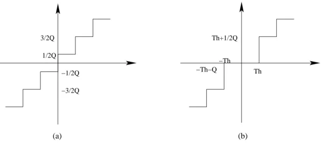
Figure 2.10 shows the quantizer characteristics in H.263. For inter DC and all AC
coefficients, input between−T h and +T h is quantized to zero. All coefficients in an MB
go through the same quantizer step sizeQ, which can be changed in increments of 2 from
2 to 62 as desired.
In the MPEG quantizer, each coefficient produced by 2D DCT is quantized with a uniform quantizer. The default quantizer matrix is defined as shown in Table 2.3, which can be changed if desired.
Furthermore, in order to provide a higher coding efficiency, a nonlinear scaler as
shown in Table 2.4 is used for the DC coefficient of 8 × 8 block in MEPG-4 video.
Note that the characteristics of nonlinear scaling are different between the luminance and chrominance blocks and depend on the quantizer used for the block.
Intra Prediction
After quantization, the DC coefficients and many AC coefficients of an intra block are coded by intra prediction (DC and AC prediction). Intra prediction is a new operation
used in MPEG-4 standards to reduce the spatial redundancy between8 × 8 blocks.
Figure 2.11 shows the prediction of DC coefficients in intra8 × 8 blocks. The
quan-tized intra coefficients are predicted with three previous decoded DC coefficients. For example, the DC coefficients of block X is predicted from the DC coefficients of blocks A, B and C. Unlike MPEG-2, the method of prediction in MPEG-4 is gradient based. In computing the prediction of block X, if the absolute value of a horizontal gradient is less than the absolute value of a vertical gradient, then the quantized DC (QDC) of block C is used as the prediction, else the QDC value of block A is used.
The AC prediction depends on DC prediction, as shown in Fig. 2.12. The AC coeffi-cients in the first row or in the first column are predicted with three previous decoded AC coefficients. The direction of prediction is the same as DC prediction.
1/2Q −1/2Q Th Th+1/2Q −Th −Th−Q (b) (a) 3/2Q −3/2Q
Figure 2.10: Quantizers in H.263. (a) For intra DC coefficient only. (b) For inter DC and all AC coefficients.
0000000000000000000000000000000000000000000
0000000000000000000000000000000000000000000
0000000000000000000000000000000000000000000
0000000000000000000000000000000000000000000
0000000000000000000000000000000000000000000
0000000000000000000000000000000000000000000
0000000000000000000000000000000000000000000
0000000000000000000000000000000000000000000
A B C D X Y Macroblock0000000
0000000
00000000000
00000
00000
00
00
or000000000000
00000000
00000000
0000
0000
0
0
orFigure 2.11: Prediction of DC coefficients of blocks in an intra MB (from [7]).
Scan and VLC
The predicted DC and AC coefficients (as well as the un-predicted AC coefficients) of DCT blocks are scanned by one of three ways: alternate-horizontal, alternate-vertical and zigzag (the normal scan used in H.263 and MPEG-1) to change the 2D image to one dimensional data, as shown in Fig. 2.13. The actual scan used depends on the coefficient prediction method used.
The coefficients after scan usually become data with many zeros at the end. This kind of data stream is good for run-length coding. In MPEG-4, differential DC coefficients in intra blocks are encoded in VLC. But the AC coefficients are encoded by the VLCs
Table 2.3: Default Quantization Matrix (Q) [5] Intra Inter 8 16 19 22 26 27 29 34 16 16 16 16 16 16 16 16 16 16 22 24 27 29 34 37 16 16 16 16 16 16 16 16 19 22 26 27 29 34 34 38 16 16 16 16 16 16 16 16 22 22 26 27 29 34 37 40 16 16 16 16 16 16 16 16 22 26 27 29 32 35 40 48 16 16 16 16 16 16 16 16 26 27 29 32 35 40 48 58 16 16 16 16 16 16 16 16 26 27 29 34 38 46 56 69 16 16 16 16 16 16 16 16 27 29 35 38 46 56 69 83 16 16 16 16 16 16 16 16
Table 2.4: Nonlinear Scaler for DC Coefficients (from [5])
Component DC Scaler forQ Range
1–4 5–8 9–24 25–31
Luminance 8 2Q Q + 8 2Q − 16
Chrominance 8 (Q + 13)/2 Q − 16
for EVENTs. An EVENT is a combination of a last non-zero coefficient indication, the number of successive zeros preceding the coded coefficient (RUN), and the non-zero value of the coded coefficient (LEVEL). Some statistically rare events have no VLC words to represent them. For them an escape coding method is used.
2.2.4
Other Video Coding Tools [7]
In addition to texture video coding, there are some special tools defined in MPEG-4. We briefly introduce robust video coding and scalable coding here.
Robust Video Coding
Error resilience is a particular concern over wireless networks. In the error resilient mode, the MPEG-4 video offers a number of tools as follows:
00000000000000000000000000000000000000000000000000000000000000000000000000000000000 00000000000000000000000000000000000000000000000000000000000000000000000000000000000 00000000000000000000000000000000000000000000000000000000000000000000000000000000000 00000000000000000000000000000000000000000000000000000000000000000000000000000000000 00000000000000000000000000000000000000000000000000000000000000000000000000000000000 00000000000000000000000000000000000000000000000000000000000000000000000000000000000 00000000000000000000000000000000000000000000000000000000000000000000000000000000000 00000000000000000000000000000000000000000000000000000000000000000000000000000000000 00000000000000000000000000000000000000000000000000000000000000000000000000000000000 00000000000000000000000000000000000000000000000000000000000000000000000000000000000 00000000000000000000000000000000000000000000000000000000000000000000000000000000000 00000000000000000000000000000000000000000000000000000000000000000000000000000000000 00000000000000000000000000000000000000000000000000000000000000000000000000000000000 00000000000000000000000000000000000000000000000000000000000000000000000000000000000 00000000000000000000000000000000000000000000000000000000000000000000000000000000000 000000 000000 00000 00000 000000 000000 00000 00000 000000 0000000000000000000000000000 00000 00000 00000 00000 00000 00000 00000 00000 00000 00000 00000 00000 00000 000000 000000 000000 000000 000000 000000 000000 000000 000000 000000 000000 000000 000000 000000 00000 00000 000000 000000 00000 00000 000000 0000000000000000000000000000 000000000000000000000000000000000000000000000000000000000000000000000000000000 A B X D C or Macroblock 000000 000000 00000 00000 000000 000000 00000 00000 00000 00000000000000000000000000000 000000 000000 000000 000000 000000 000000 000000 000000 000000 000000 000000 000000 000000 Y or
Figure 2.12: Prediction of AC coefficients of blocks in an intra MB (from [7]).
Figure 2.13: Scans for8 × 8 blocks (from [5]).
1. Object priorities: The object based organization of MPEG-4 video facilitates priori-tizing of the semantic objects based on their relevance. Further, the VOP types are a form of inherent prioritization since B-VOPs do not contribute to error propagation and thus can be transmitted at a lower priority or discarded in case of severe errors. 2. Resynchronization: The encoder can enhance error resilience by placing resynchro-nization (resync) markers in the bitstream with approximately constant spacing, such as beginning of each MB.
3. Data partitioning: Data partitioning provides a mechanism to increase error re-silience by separating the normal motion and texture data of all MBs in a video packet and send all of the motion data followed by a motion marker, followed by
all of the texture data.
4. Reversible VLCs: The reversible VLCs offer a mechanism for a decoder to recover additional texture data in the presence of errors since the special design of reversible VLCs enables decoding of codewords in both the forward (normal) and the reverse directions.
5. Intra update and scalable coding: To prevent error propagation, intra update is a simple method to solve the problem. However, intra coding will reduce the coding efficiency. Another method is scalable coding, which can prevent error propagation without more intra coding.
Scalable Coding
The scalability tools in MPEG-4 video are designed to support applications beyond that supported by single layer video, such as internet video, wireless video, multi-quality video services, video database browsing, etc. In scalable video coding, it is assumed that given a coded bitstream, decoders of various complexities can decode and display appropriate reproductions of coded video.
Several different forms of scalability are provided in MPEG-4 video. Temporal and spatial scalability are the most basic scalability tools among them. A Fine Granularity Scalability (FGS) is also defined which supports continuous scalability of bit rate and video quality.
2.3
Profiles and Levels [5]
Although there are many tools in the MPEG-4 standard, not every MPEG-4 decoder will have to implement all of them. Similar to MPEG-2, profiles and levels are defined as subsets of the entire bitstreams syntax of all the tools. The purpose of defining confor-mance points in the form of profiles and levels is to facilitate interchange of bitstreams among different applications. There are eight profiles defined in MPEG-4: simple, core,
main, simple scalable, animated & mesh, basic animated texture, still scalable texture, and simple face. The details are given in Table 2.5.
Compared with previous standards, the simple profile of MPEG-4 is similar to the coding method in H.263. The difference is that the simple profile has error resilience but does not have B-frame coding. The simple scalable profile is simple profile with rectangular scalability. The core profile is the profile with all tools of the simple profile, temporal scalability, B-VOP coding and binary shape coding. The main profile is the profile with all tools in core profile, gray shape coding, interlace and sprite coding. The other profiles are for particular purposes, such as 2D dynamic mesh coding and facial animation coding.
Table 2.5: Profiles and Tools (from [5])
Simple Core Main Simple Animated Basic Still Simple Tools Scalable 2D Mesh Animated Scalable Face
Texture Texture Basic 1. I VOP 2. P VOP V V V V V 3. AC/DC Prediction 4. 4MV Unrestricted MV Error resilience 1. Slice Resynchronization V V V V V 2. Data Partitioning 3. Reversible VLC Short Header V V V V B-VOP V V V V Method 1/Method 2 V V V quantization P-VOP based temporal scalability 1. Rectangular V V V 2. Arbitrary Shape Binary Shape V V V Gray Shape V Interlace V Sprite V Temporal scalability V (rectangular) Spatial scalability V (rectangular) Scalable still V V V texture 2D dynamic mesh V V
with uniform topology
2D dynamic mesh V
with Delaunay topology
Facial animation V
Chapter 3
Overview of PACDSP
The contents of this chapter have been taken to a large extent from [1].
We consider implementation of MPEG-4 object-based video decoder on the PACDSP version 2.0. We focus on introducing it in this chapter. In the last section, we give a brief introduction to version 3.0, which is the latest version of the PACDSP.
3.1
Introduction
For high performance, the PACDSP is a VLIW processor with single instruction multiple data (SIMD) instruction set architecture (ISA). The software supported reducing hard-ware design complexity and power consumption. Variable length instruction and instruc-tion packet solve the poor code density problem of the conveninstruc-tional VLIW architecture. Another feature of the PACDSP, cluster architecture, reduces not only ports of the reg-ister files but also the power consumption of read/write operations. Key features of the PACDSP include the following items:
• Scalable VLIW datapath for easy extension of the performance.
• Variable instruction word/packet length to avoid the drawback of poor code density
in the conventional VLIW architecture.
• Heterogeneous register files for more straightforward operations, less ports and
and area.
• Constant register file in each cluster (32×32 bits) for storage of some fixed data in
the applications to reduce the frequency of data movement which may cost signifi-cant power consumption.
• Inter-cluster communication by memory controller for reusing hardware resource
and reducing the port number of ping-pong register file in order to reduce power and area and to increase the scalability.
• Optimized interrupt design with fast interrupt response time (3 clock cycles) with
hardware supported context switch to reduce the processing time of interrupt service routine (ISR).
• Hierarchical encoding scheme reducing the dependency between instructions and
packets to reduce area and latency of the dispatch unit.
• Dynamic power management for power saving.
• Customized instruction set and functional unit interface for the accelerators that are
used to enhance certain DSP operations.
There are three components in the PACDSP kernel: program sequence control unit, scalar unit and VLIW datapath. The accelerators that execute in different threads and synchronize the execution results through the scalar unit can enhance the computation power of the VLIW datapath. Figure 3.1 shows the architecture of the PACDSP.
3.2
Program Sequence Control Unit
The program sequence control unit is a main component in the DSP kernel. It dispatches instructions to the scalar unit and the VLIW datapath. It also executes the execution flow control instructions and handles the interrupt and exception events.
Figure 3.1: Architecture of the PACDSP (from [1]).
3.2.1
Branch Instructions
Branch instructions can be grouped into two categories, conditional branches and uncon-ditional branches. There are three addressing modes defined in the PACDSP for generat-ing the branch target address:
• Program counter (PC)-relative
Add the 16-bit signed immediate offset to the address in the PC register, and take the result as the branch target address, i.e.,
TA = PC + OFFSET
where TA is the target address, PC is the address in PC register, and OFFSET is the 16-bit signed immediate value defined in branch instruction.
• Register
TA = Rs
where TA is the target address and Rs is the source register of address.
• Register-relative
Add the 16-bit signed immediate offset to the address saved in the register and take the result as the branch target address, i.e.,
TA = Rs + OFFSET
where TA is the target address, Rs is the source register saving the address, OFFSET is the 16-bit signed immediate value.
The branch instructions defined in the PACDSP support saving of the return address into the assigned register. The programmer should take care of the return addresses of nested loops. There are three branch delay slots in the PACDSP, and independent instruc-tions can be put in these delay slots.
3.2.2
Loop
The programmer can use the LBCB instruction to effect program loops. Loop Boundary Registers (RBC0 – RBC3), which are all 32-bit registers, can be used to record the loop counts. However, the maximum loop count is 65,536 for each level. Since there are four Loop Boundary Registers, up to four levels of nested loop can be supported with the use of the LBCB instruction.
A constraint exists in using LBCB to control a nested loop, that is, the outer loop should fully contain the inner loop. No exception will be generated if the constraints are violated, but the program behavior may be different from expectation.
However, conditional branches can be used inside the nested loop to implement some special branch behaviors in higher level languages, for example, “break” and “continue” in C.
3.2.3
Customized Function Units
The PACDSP provides Customized Function Unit Interface for extension purpose. The user can attach co-processors or customized function units to PACDSP and handle them through the scalar instructions. If some error happens in a customized function unit, it can inform the PACDSP and the PACDSP can process it based on the particular configuration. If the work given is finished successfully, the PACDSP can use its results and continue to work. It is recommended to use this interface to communicate with any added co-processor; otherwise, the user may have to pay significantly more effort to handle it.
3.2.4
Exception Handling
Unpredictable exceptions may occur during program execution. The exceptions need to be handled correctly for correct execution results. Exceptions may be caused by hard-ware (e.g., overflow), softhard-ware, internal (e.g., undefined instruction), or external (e.g., coprocessor exception). When an exception happens, the DSP kernel will be frozen or listen to the main processing unit (MPU). It is still aware of debug requests and will check the corresponding signal to see what kind of exceptions have happened.
3.2.5
Interrupt Handling
Two types of interrupt are supported by the PACDSP. One is fast interrupt request (FIQ), which has the higher priority, and the second is interrupt request (IRQ). The difference between them is that the FIQ uses hardware to reduce the time in saving the context and the hardware resources used for the FIQ interrupt service routine (ISR) consist only of the scalar unit and program sequence control unit. In contrast, the IRQ can use all the hardware resources in PACDSP to deal with the IRQ request, but the ISR of IRQ needs to save the context by itself.
In the PACDSP, the minimum latency from interrupt request to the first ISR instruction to be executed is 3 cycles for both types of interrupt, and it may be postponed when the ISR experiences cache miss.
3.3
VLIW Datapath
The VLIW datapath is composed of two clusters which takes charge of complex data oper-ations in the program. Each cluster contains a load/store unit (L/S) and an arithmetic unit (AU). Both units can execute instructions concurrently. Another feature of the PACDSP, the ping-pong register file, facilitates data transfers between these two units. With this feature, the typically high power consumption of the DSP kernel can be reduced. The maximum parallelism of the VLIW datapath in instruction and operation levels is 4 and 12, respectively.
3.3.1
Arithmetic Unit (AU)
The arithmetic unit (AU) comprises four 40-bit adders which can be reconfigured to two 16-bit adders or four 8-bit adders, two 16-bit multipliers, one shifter and one logical ALU. All data processing instructions in AU begin at the same stage, but not finish at the same time.
There are three types of precision in DSP — full, integer, and fractional. Figure 3.2 shows how it works.
• Full precision: Rd = Rs1.L × Rs2.L. • Integer: Rd.L = (Rs1.L × Rs2.L)[15:0]. • Fractional: Rd.L = Rs1.L × Rs2.L)[30:15].
3.3.2
Load/Store Unit (L/S)
The load/store unit (L/S) comprises one address generation unit (AGU), one logical ALU, and one shifter. Similar to AU, all instructions in L/S begin at the same stage, but not finish at the same time.
The L/S unit supports powerful double load/store instructions, which can load or store two operands in one instruction. Figure 3.3 shows how double and vector load/store work.
00 00 00 00 11 11 11 11 000000000000000000 000000000000000000 000000000000000000 000000000000000000 111111111111111111 111111111111111111 111111111111111111 111111111111111111 000000000000000000 000000000000000000 000000000000000000 111111111111111111 111111111111111111 111111111111111111 Full Precision Integer Fractional Rs2.L Rs1.L Rd.L Rs1.L Rs1.L Rd.H Rd.L Rd.L Rs2.L Rs2.L
Figure 3.2: Illustration of multiplication instructions with different precisions (from [1]).
3.3.3
Ping-Pong Register File
A centralized register file (RF) provides storage for and interconnects to each functional unit (FU), and each FU can read from or write to any register location. But in practical designs, the communication between FU is usually restricted by partitioning the RF to reduce the complexity significantly with some performance penalty. In other words, each FU can only read and write a limited subset of registers. In the ping-pong hierarchical RF, which is shown in Fig. 3.4, the RF is partitioned into private and ping-pong sub-blocks. Each FU (L/S or AU) can simultaneously access two sub-blocks, one of which is private (i.e., dedicated to the FU) and the other is dynamically mapped for inter-FU communications within one cluster. Therefore, each sub-block only requires the access ports for a single FU. The shared sub-blocks are organized in a ping-pong fashion to reduce the control overhead, where the dynamic mapping is exposed to the VLIW ISA with two switching bits and is directly specified by the programmers for each instruction
D1 D3 D5 D7 D0.L D1.L D2.H D0 D2 D4 D6 D0.H D1.H D3.H D2.L D3.L
Unit
Load/Store
Unit
Load/Store
Double
Load//Store
Load/Store
Vector
Figure 3.3: Different load/store instructions (from [1]). packet.
3.3.4
Data/Address/Accumulator Registers
As shown in Fig. 3.5, the address registers (A0–A7) are all 32-bit and they are dedicated to the load/store unit (L/S) for memory accesses. In addition, A1, A3, A5, and A7 are also treated as the base registers which contain the base addresses in modulo addressing mode. E0–E3 (A8, A10, A12, and A14) and D0–D3 (A9, A11, A13, and A15) are individually treated as end registers and displacement registers which contain end addresses and dis-placements in modulo addressing mode. Nevertheless, in linear addressing mode, they can be treated as the address register like A0–A7. The accumulator registers (AC0–AC7) are 40-bit (8 guard bits) and are dedicated to the arithmetic unit (AU) for data manipula-tions. The data registers (D0–D7 and D8–D15) are organized in the form of ping-pong with 1-bit control and the word-length of these registers is 32.
A0 − A15 (32−bit)
Private Registers
D0 − D7 (32−bit)
Ping−Pong Register
D8 − D15 (32−bit)
AC0 − AC7 (40−bit)
Private Registers L/S
AU
2−bit configuration
Figure 3.4: Ping-pong register file in one cluster (from [1]).
3.3.5
Status and Control Registers
The status register and control register which can be read and set by user instructions can be used to monitor the DSP kernel status and handle the operation mode of DSP kernel.
Program Status Register (PSR)
The 16-bit program status register records the operation status in each cluster and the scalar unit. It includes Overflow, Negative, and Carry bits. It can only be read by user instructions.
Addressing Mode Control Register (AMCR)
D11.H D13.H D14.H AC1.H AC6.H AC7.H AC0.L AC1.L A9/D0 Data Register 32−bit (L/S) Data Register 32−bit (AU) Accumulater Register 40−bit (AU) Address Register 32−bit (L/S) End/Displacement Register 32−bit (L/S) AC1.G AC2.G AC3.G AC4.G AC5.G AC7.G D0.H D1.H D2.H D3.H D4.H D5.H D6.H D7.H D0.L D1.L D2.L D3.L D4.L D5.L D6.L D7.L D8.H D9.H D10.H D12.H D15.H D8.L D9.L D10.L D11.L D12.L D13.L D14.L D15.L AC0.GAC0.H AC2.H AC4.H AC3.H AC5.H AC6.G AC6.L AC5.L AC4.L AC3.L AC2.L AC7.L A0 A2 A4 A6 A1/B0 A3/B1 A7/B3 A5/B2 A8/E0 A10/E1 A12/E2 A14/E3 A11/D1 A13/D2 A15/D3
Figure 3.5: Available registers in one cluster (from [1]).
• Linear addressing mode. • Bit-reverse addressing mode. • Modulo addressing mode.
The addressing mode control register (AMCR) is a 32-bit read/write register. This reg-ister is used to control the addressing mode of relative address regreg-isters. The addressing modes are related to where the operands are to be found and how the address calculations are to be made.
3.3.6
Addressing Modes
The addressing modes are related to where the operands are to be found and how the address calculations are to be made.
Linear Addressing Mode
There are three kinds of linear addressing mode, which are register direct mode, address register indirect mode, and immediate data mode. These are briefly explained below.
1. Register direct mode: This mode specifies that the operand is in one or more of the arithmetic unit (AU) registers, load/store unit (L/S) registers, control registers and program counter (PC) registers. It is also used to specify a control register operand and a PC register operand for special instructions.
2. Address register indirect mode: This mode specifies that the address register is used to point to a memory location. The term indirect is used because the register contents are not the operand itself, but the operand address. This addressing mode specifies that an operand is in a memory location and specifies the effective address of that operand. There are still two sub-modes in the address register indirect mode:
• Pre-increment, +(Rs) offset
The operand address is the sum of the contents of the address register and the offset. The data stored at the address of the sum of register value and offset will be loaded.
• Post-increment, (Rs)+ offset
The operand is in the address register Rs. After the operand address is used, it is incremented by the offset and stored in the same address register. Incre-menting the operand address by the offset places the next available address in the register. That is, the data stored at the location of the address register will be loaded first, and then the address is updated with the offset.
3. Immediate data mode: This mode does not use an address register. The instructions use an immediate value that is included in the instruction for the data value or address value.
Bit-Reverse Addressing Mode
Bit-reverse addressing mode is also called reverse-carry addressing mode. It is useful for
2k-point fast fourier transform (FFT) addressing. This mode is selected by setting the
corresponding bits in AMCR, and address modification is performed in the hardware by propagating the carry from each pair of added bits in the reverse direction (from the MSB end toward the LSB end). It can also use the pre- or post-increment addressing mode.
This address modification is useful for addressing the twiddle factors in 2k point-FFT addressing as well as to unscramble2k-point FFT data.
Modulo Addressing Mode
Modulo address modification is useful for creating circular buffers for FIFO queues, delay lines, and sample buffers.
The definition of modulo addressing, using a base register (Bn) and a modulo register
(Mi), enables the programmer to locate the modulo buffer at any address. The address
pointer,An, is not required to start at the lower address boundary, nor to end on the upper address boundary. It can initially point to anywhere (aligned to its access width) within
the defined modulo address range,Bn ≤ An < Bn + Mi.
Modulo addressing can be selected by configuring corresponding bits in AMCR and
write the desired modulo to modulo registers. The range of modulo registers,Mi, is from
1 to232− 1.
Each base address register (Bn) is associated with an address register. Offset and
modifier registers are also associated with the corresponding address registers in the same way.
3.3.7
Data Exchange
As shown in Fig. 3.6, the PACDSP provides a data exchange mechanism between any two of the scalar unit and the two clusters. Figure 3.7 shows that it can also provide data broadcast to facilitate one of them to broadcast its data to the others even though the number of clusters may be extended in the future. This job is accomplished by using the ports of the memory interface unit (MIU) because MIU has connections with all register files of the scalar unit and the two clusters.
Data Exchange Between Clusters
The PACDSP provides a special instruction (DEX) to accomplish data exchange between clusters. For example:
Unit Load/Store Unit Arithmetic Cluster1 Unit Load/Store Unit Arithmetic Cluster2 M I U Scalar Unit
Figure 3.6: Data exchange between two clusters (from [1]).
Unit Load/Store Unit Arithmetic Cluster1 Unit Load/Store Unit Arithmetic Cluster2 M I U Scalar Unit
Figure 3.7: Data broadcast among clusters (from [1]). Cluster1 instruction: DEX D1, D0
Cluster2 instruction: DEX D1, D2
At compile time, this instruction pair will cause direct exchange of the contents of D0 and D2 through MIU and each cluster will store them in D1, as shown in Fig. 3.6.
Data Broadcast
Like data exchange between clusters, PACDSP also provides a special instruction pair (BDT and BDR) for data broadcast from one cluster to the others. For example:
Cluster1 instruction: BDT D0 Cluster2 instruction: BDR D3
Scalar instruction: BDR R0
At compile time, this set of instructions will broadcast data from cluster1 to cluster2 and the scalar unit as shown in Fig. 3.7.
On the other hand, if we just want to transmit data from one cluster to another (includ-ing the scalar unit), it can be considered a special case of data broadcast. For example: Cluster1 instruction: ADD D0, D1, D2
Cluster2 instruction: BDR D7 Scalar instruction: BDT R0
In this example, the content of R0 is transmitted to D7 in cluster2. At the same time, cluster1 can do other operations without interference with this transmission.
3.3.8
Constant Register File
In many DSP algorithms, such digital filtering, there are many fixed data such as the filter coefficient. In order to avoid high frequency of data movement in the register file, the PACDSP provides a small memory called Constant Register File to maintain the fixed data. We can also use it to store look up tables which contain fixed data for specific applications. It can reduce the frequency of data movement and thereby reduce power consumption in such operations.
Data contained in the Constant Register File can be used in comparisons, multiplica-tions, multiplications and accumulamultiplica-tions, etc. They are used as the second source operand in the instructions.
The specifications of Constant Register File (in one cluster) are as follows:
• 32 × 32 bits.
• Two read ports and one write port.
As shown in Fig. 3.8, the Constant Register File is initialized through the write port by MIU at the beginning of the program. Not only the L/S but also the AU has a read port for taking its value as one source operand. There are some rules when using the Constant Register File:
• It can only be modified by particular instructions in L/S.
• Read and write operations may not occur at the same time in L/S.
3.4
Scalar Unit
The scalar unit executes the scalar instructions whose characteristics are low parallelism and high data dependency. It also controls the power control interface and the customized functional unit interface.
3.4.1
Scalar Unit
The Scalar Unit can perform three types of function, which are basic arithmetic oations, word and halfword-based load/store operoations, and read/write operations per-formed on the control/status registers. Under some running modes, the DSP core may execute a program without activating the VLIW clusters. In this case, the scalar unit acts like a simple machine, handling some easy tasks. Mostly, the scalar unit is in charge of the control-based work while the VLIW clusters are dealing with data processing. Data can be exchanged between the scalar unit and the VLIW clusters.
3.4.2
Control Registers
In the PACDSP kernel, there are 15 control registers. Table 3.1 shows the names and the widths of all the control registers in the PACDSP kernel.
Several control registers are memory mapped and can be accessed by others outside the PACDSP kernel. Table 3.2 lists the memory mapped control registers and the mapping memory addresses.
The control registers can be read or write by the scalar instructions. When writing the control registers, we can assign a 16-bit immediate value to the destination or set a general purpose scalar register as the source operand.
Load/Store Unit Customized FU Public Ping−Pong RF Customized FU Private RF Private RF
Memory
Coefficient
Memory Interface Unit (MIU)
Arithmetic Unit
Figure 3.8: The Constant Register File of one cluster (from [1]).
3.4.3
General Purpose Scalar Register File
In the scalar unit of the PACDSP kernel, there are sixteen 32-bit general purpose registers named R0 to R15.
3.5
Conditional Execution Control
Unlike general purpose processors, the major mission of a DSP is to provide more com-puting power for numerical calculations. To reduce control overhead, the PACDSP sup-ports conditional execution of instructions. Programmers can set predicates by Compare-and-Set instructions and then the instructions afterward can refer to the predicates to de-cide whether to execute or not. When the program calls a function, we can save the predicates and restore them after returning from the function call.
![Figure 2.2: Structure of coded video data (from [8]). 1. An intra-coded (I) VOP is coded using information only from itself.](https://thumb-ap.123doks.com/thumbv2/9libinfo/7682913.142402/23.918.190.701.86.479/figure-structure-coded-video-intra-coded-coded-information.webp)
![Table 2.1: List of BAB Types (from [5]) BAB Types Semantic Used in](https://thumb-ap.123doks.com/thumbv2/9libinfo/7682913.142402/27.918.206.690.97.366/table-list-bab-types-bab-types-semantic-used.webp)
![Figure 2.7: Simplified padding process (from [5]). matching to handle arbitrary-shaped VOPs which is block-based method.](https://thumb-ap.123doks.com/thumbv2/9libinfo/7682913.142402/29.918.229.672.104.659/figure-simplified-padding-process-matching-handle-arbitrary-shaped.webp)
![Figure 3.6: Data exchange between two clusters (from [1]).](https://thumb-ap.123doks.com/thumbv2/9libinfo/7682913.142402/53.918.192.702.84.327/figure-data-exchange-clusters.webp)
![Table 3.2: Memory-Mapped Control Registers (from [1])](https://thumb-ap.123doks.com/thumbv2/9libinfo/7682913.142402/58.918.164.731.108.336/table-memory-mapped-control-registers-from.webp)
![Table 3.4: Running Modes of the PACDSP (from [1])](https://thumb-ap.123doks.com/thumbv2/9libinfo/7682913.142402/61.918.126.786.139.669/table-running-modes-pacdsp.webp)
![Figure 3.15: Architecture of PACDSP v3.0 (from [2]).](https://thumb-ap.123doks.com/thumbv2/9libinfo/7682913.142402/66.918.183.711.100.438/figure-architecture-of-pacdsp-v-from.webp)
![Figure 4.1: Block diagram of MPEG-4 object-based video decoder [5].](https://thumb-ap.123doks.com/thumbv2/9libinfo/7682913.142402/70.918.177.722.110.617/figure-block-diagram-mpeg-object-based-video-decoder.webp)
