Regular and chaotic dynamic analysis and control of chaos of an elliptical pendulum on a vibrating basement

doi:10.1006/1999.2664, available online at http://www.idealibrary.com on

REGULAR AND CHAOTIC DYNAMIC ANALYSIS AND

CONTROL OF CHAOS OF AN ELLIPTICAL PENDULUM

ON A VIBRATING BASEMENT

Z.-M. GE AND T.-N. LIN

Department of Mechanical Engineering, National Chiao ¹ung ;niversity, Hsinchu, ¹aiwan, Republic of China

(Received 22 July 1998, and in ,nal form 3 September 1999)

The dynamic behavior of an elliptical pendulum subjected to external disturbance is studied in this paper. The Lyapunov direct method is applied to obtain conditions of stability of the equilibrium points of the system. By applying numerical results, phase diagrams, power spectrum, period-T maps, and Lyapunov exponents are presented to observe periodic and chaotic motions. The e!ect of the parameters changed in the system can be found in the bifurcation and parametric diagrams. For global analysis, the basins of attraction of each attractor of the system are located by employing the modi"ed interpolated cell mapping (MICM) method. Finally, several methods, the delayed feedback control, the addition of constant torque, the addition of periodic force, adaptive control algorithm and bang-bang control are used to control chaos e!ectively.

( 2000 Academic Press

1. INTRODUCTION

In the past one and a half decade, a large number of studies have shown that chaotic phenomena are observed in many physical systems that possess non-linearity [1, 2]. It was also reported that the chaotic motion occurred in many non-linear control systems [3, 4]. Many studies of the pendulum have been accomplished in recent years [5, 6]. This paper will study the non-linear behavior of an elliptical pendulum system.

A lot of modern techniques are used in analyzing the deterministic non-linear system behavior. Both analytical and computational methods are employed to obtain the characteristics of the non-linear systems. The Lyapunov direct method is applied to obtain conditions of stability of the equilibrium points of the system. By applying numerical results, phase diagrams, power spectrum, period-¹ maps, and Lyapunov exponents are presented to observe periodic and chaotic motions. The e!ect of the parameters changed in the system can be found in the bifurcation and parametric diagrams. For global analysis the basins of attraction of each attractor of the system are located by employing the modi"ed interpolated cell mapping (MICM) method. Finally, attention is shifted to the controlling of chaos. For this

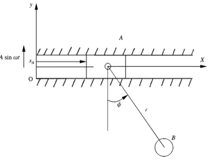
Figure 1. System model.

purpose, the delayed feedback control, the addition to constant torque, the addition periodic force, adaptive control algorithm (ACA) control and bang-bang control are used to control chaos.

2. EQUATIONS OF MOTION

The system considered here is depicted in Figure 1. A block connecting a particle can slide on a "xed horizontal plane. It is a pendulum system and so the mass of the connecting rod can be neglected, and the pendulum can be assumed as a particle. The pendulum swings on an x}y plane. Then Lagrange's equations of motion can be expressed as follows:

d

dt[(mA#mB)xRA#mBl/Qcos /]"0, (2.1)

d

dt(mB l2 /Q#mBlxRAcos /)#mBlxRA /Qsin/"!mBgl sin/, (2.2) where mA is the mass of the block, mB is the mass of the pendulum, xA is the displacement of the block,/ is the angle between the y-axis and the pendulum, and l is the length between the block and the pendulum. From Equation (2.1), it could be rewritten as

(mA#mB) xRA#mB l/Qcos /"c1. (2.3)

Equation (2.3) is a "rst integral and c1 is an arbitrary constant. When t"0, xA"0, xR A"0, /"/0, /"0. Substituting these initial conditions into equation (2.3), and c1"0, equation (2.3) becomes

or

xR A"! mB

mA#mBl/Q cos /. After integration, we get

xR A"! mB

mA#mB l sin/#c2 From the above initial conditions, c2 can be written as

c2"_mA#mBmB l sin/0. Then xA can be written as

xA"_mA#mBmB l (sin/0!sin/). (2.5) The parametric equations of the locus of the pendulum can be written as

xB"xA#l sin/"_mA#mBmB l (sin/0!sin/)#lsin/ "

c2#_mA#mBmA l sin/, yB"!lcos /.

By eliminating the parameter/, the equation of the locus of the pendulum can be expressed as

A

B

2

(xB!c2)2#y2B"l2.

This is an equation of ellipse, therefore the pendulum is called elliptical pendulum [6].

By considering the damping e!ect, the equations of motion can be expressed as (mA#mB)xKA#mB l /Gcos /!mB l /Q2 sin /"!k2xRA,

mB l2 /G#mB l xKA cos /#mBgl sin /"!k1/Q, (2.6) where k1 and k2 are the damping constants.

Let xA"x1, xRA"x2, /"x3, /Q"x4, and change the time t to dimensionless timeq"Xt. The state equations can be written as

x5 1"x2

xR 2" l sin x3

(a!cos2 x3)x24#X2 (a!cos2 x3)g sin x3 cos x3 !XmB(a!cos2x3)k2 x2 # k1 cos x3

x5 3"x4,

xR 4" !ag sin x3

X2 l (a!cos2 x3)!(a!cossin x3cos x32 x3) x24!XmBl2(a!cos2x3)ak1 x4

# k2 cosx3 XmBl(a!cos2x3) x2, (2.7) where a"mA#mB mB , X" 1 2n

S

in whichX is the natural frequency of the small vibration of the undamped system which can be derived as follows. From equations (2.1), (2.2), and (2.4), and eliminating xRA, we have

A

mA#mB

B

lsin/"0. (2.8) When the vibration is small, sin/+/, cos /+1, the higher order terms can be neglected, Equation (2.8) can be rewritten as

/G#

A

B

g

l /"0 (2.9)

and the natural frequency for linear vibration isX"(1/2n) J(mA#mB)g/mAl.

3. STABILITY ANALYSIS BY LYAPUNOV DIRECT METHOD

The stability of the motion of the system will be investigated by Lyapunov's direct method in this section. Since x1 does not appear on the right-hand side of equation (2.7), we may consider a three-dimensional case:

xR 2" l sin x3

(a!cos2 x3)x24#X2 (a!cos2 x3)g sin x3 cos x3 !XmB(a!cos2x3)k2 x2 # k1 cos x3

XmBl(a!cos2x3)x4, xR 3"x4,

xR 4" !ag sin x3

X2 l (A!cos2 x3)!(a!cossin x3cosx32 x3) x24!XmBl2 (a!cos2x3)ak1 x4 # k2 cos x3

The equilibrium position (0, 0, 0) is a solution of equation (3.1) the stability of which we shall study. Equation (3.1) is the state equations for disturbances. By Taylor series expansion, it becomes

xR 2"_{X2 (a!1)x3#}g k1

XlmB(a!1) x4!XmB(a!1)k2 x2#2, xR 3"x4,

xR 4" k2

XmBl(a!1)x2!XmBl2(a!1)ak1 x4! ag

X2 l (a!1)x3#2. (3.2) The higher order terms are not presented but not neglected. Construct a Lyapunov function as

<"x22#x23#x24#x3x4. (3.3)

<_{is the positive-de"nite function and the derivative of < through equation (3.3) is}

d< dt"

C

D

C

X2 (a!1)#2XmBl(a!1)k2 XmBl(a!1)k1#k2

g

X2 (a!1)#2XmBl(a!1)k2

!ag

X2 l (a!1) 1! ag

X2 l (a!1)!2XmBl2 (a!1)ak1

k1#k2

XmBl(a!1) 1! ag

X2 l (a!1)!2XmBl2 (a!1)ak1 1!XmBl2(a!1)2ak1

D

C

D

#2. (3.4)

By Sylvester's theorem, the derivative of < is negative de"nite if ! 2k2 XmB(a!1)(0, (3.5a) 8aXmBlk2g!8XmBlk2g!4m2Bl2g2!k22'0, (3.5b) 2ak2gX2m2Bl3(a!1)!4XmBl#2g(k1#k2)X2m2B l3 (a!1)!agk1 (k1#k2)XmBl # k2(k1#k2)X3mBl2(a!1)!k2ag(k1#k2)XmBl!2ag2(k1#k2)m2Bl2 (a!1) !1 2ak1k2(k1#k2)X2#ag(k1#k2)2XmBl#2k2X4m2Bl4(a!1)2#2a2 g2k2m2B l2

#1

2a2k21k2X2(a!1)!4agk2X2m2Bl3(a!1)#2a2gk1k2XmBl!2k1k2X3mBl2(a!1) #

2ak1gX2m2Bl2 (a!1)2#ak1k2X3mB l (a!1)!gX3m3Bl4 (a!1)2

!1

2k2X4m2Bl3 (a!1)2(0. (3.5)

By Lyapunov's theorem of asymptotical stability [2], equation (3.5) are the conditions of the asymptotical stability of zero solution of the elliptical pendulum system.

In the above analysis, the angular damping k1 is assumed to be constant in, e.g. equation (3.1), for which when external excitation is added, no chaotic dynamics can be found. Therefore, another condition will be studied later on; the angular damping is not constant but is represented by a van der Pol term k1 (x23!1). Then the dynamic equations (2.7) become

xR 1"x2, xR 2" l sin x3

(a!cos2 x3)x24#X2 (a!cos2 x3)g sin x3 cos x3 !XmB(a!cos2x3)k2 x2 # k1(x23!1) cosx3

XmBl(a!cos2x3)x4, xR 3"x4,

xR 4" !ag sin x3

X2l(a!cos2 x3)!(a!cossin x3cos x32 x3)x24!XmBl2(a!cos2x3)ak1 (x23!1) x4

# k2cos x3

XmBl(a!cos2x3)x2. (3.6)

Since x1 also does not appear on the right-hand side of equation (3.6), we may use the last three equations of equation (3.6) to study the stability of x2, x3, x4 similar to what we have done for equation (3.1). Also, by Taylor series expansion, the last three equations of equation (3.6) become

xR 2" g

X2 (a!1)x3!_XlmB(a!1)k1 x4!_XmB(a!1)k2 x2#2, xR 3"x4,

x_{R 4"} k2

XmBl(a!1)x2#XmBl2(a!1)ak1 x4! ag

X2 l (a!1)x3#2. (3.7) The characteristic equation is

j3# k2l2!ak1

XmBl2(a!1)j2#

A

X2l (a!1)!_X2l2m2B(a!1)k1k2

B

By Lyapunov's "rst approximation theory [7] and the Routh}Hurwitz criterion, zero solution of the non-linear system consisting of the last three equations of equation (3.6) is asymptotically stable if

k2 l2!ak1'0, ag

X2l (a!1)!_X2l2m2B(a!1)k1k2 !_X2(k2l2!ak1)k2gl '0, k2g

X3mB l(a!1)'0, (3.9)

which are quite di!erent from those for the system with linear damping, equation (3.5).

4. PHASE PORTRAITS, PERIOD-T MAP AND POWER SPECTRUM For the system with van der Pol damping, because of the vertical vibration A sinut of the horizontal plane, the co-ordinate system "xed with the plane becomes a non-inertial system. Adding the inertial force term to the constant gravity term of the pendulum particle, the gravity of the pendulum particle is now represented by a constant term and a harmonic term g!Au2 sin ut, where g, A, u, k1, k2 are constants. The Lagrange dynamic equation for the non-inertial system becomes

xR 1"x2, xR 2" l sin x3

(a!cos2 x3)x24#X2 (a!cos2 x3)g sin x3 cos x3 !XmB(a!cos2x3)k2 x2 # k1(x23!1) cosx3 XmBl(a!cos2x3)x4! Au2 sin x3cosx3 X2 (a!cos2 x3) sin u X q, xR 3"x4, xR 4" !ag sin x3

X2 l (a!cos2 x3)!(a!cossin x3cos x32 x3) x24!XmBl2(a!cos2x3)ak1 (x23!1) x4

# k2cos x3 XmBl(a!cos2x3)x2# Aau2 sin x3 X2 l (a!cos2 x3) sin u Xq, (4.1)

where a"3)0, g"9)8,X"0)863, k1"0)25, k2"0)3, mB"1, u"1, l"0)5. The last terms of the right-hand sides of the second and fourth equations in equation (4.1) are the excitation terms.

The phase plane is the evolution of a set of trajectories emanating from various initial conditions in the state space. When the solution reaches a stable state, the asymptotic behavior of the phase trajectories is particularly interesting and the transient behavior in the system is neglected. The period-¹ map, where ¹ is the time period of the forcing is a better method for displaying the dynamics. Equation (4.1) is plotted in Figures 2(a) and 2(b) for A"12)4 and 12)5, respectively. Clearly,

Figure 2. Phase portrait and period-¹ map &&_{3 '' for (a) A}"12)4, (b) A"12)5, (c) A"12)6, phase portraits of chaos, (d) period-¹ map && ) ''.

the motion is periodic. But Figures 2(c) and 2(d) for A"12)6 show the chaotic state. The points of the period-¹ map become irregular.

Another technique for the identi"cation and characterization of the system is power spectrum. It is often used to distinguish between periodic, quasi-periodic and chaotic behavior for a dynamical system. Any function x(t) may be represented as a superposition of di!erent periodic components. The determination of their relative strength is called spectral analysis. If it is periodic, the spectrum may be a linear combination of oscillations whose frequencies are integer multiples of basic frequency. The linear combination is called a Fourier series. If it is not periodic, the spectrum then must be in terms of oscillations with a continuum of frequencies. Such a representation of the spectrum is called Fourier integral of x(t). The representation is useful for dynamical analysis. The non-autonomous system is observed by the portraits of power spectrum in Figures 3(a) and 3(b) for period-¹ and period-2¹ steady state vibration. As A"12)6 chaos occurs, the spectrum is a broadband as shown in Figures 3(c) and 3(d). The noise-like spectrum is the characteristic of a chaotic dynamical system.

5. BIFURCATION DIAGRAM AND PARAMETER DIAGRAM

In the previous section, the information about the dynamics of the non-linear system for speci"c values of the parameters is provided. The dynamics may be viewed more completely over a range of parameter values. As the parameter is changed, the equilibrium points and periodic motions can be created or destroyed, or their stability can be lost. The phenomenon of sudden change in the motion as a parameter is varied is called bifurcation, and the parameter values at which they occur are called bifurcation points. The bifurcation diagram of the non-linear system of equation is depicted in Figure 4. A 3 [12)4, 12)6] with the incremental value of A being 0)0001.

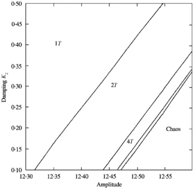
Further, the parameter value and damping coe$cient will also be varied to observe the behaviors of bifurcation of the system. Parameter diagrams are shown in Figure 5.

6. LYAPUNOV EXPONENT AND LYAPUNOV DIMENSION

The Lyapunov exponent may be used to measure the sensitive dependence upon initial conditions. It is an index for chaotic behavior. Di!erent solutions of a dynamic system, such as "xed points, periodic motions, quasiperiodic motion, and chaotic motion can be distinguished by it. If two trajectories start close to one another in phase space, they will move exponentially away from each other for small times on the average. Thus, if d0 is a measure of the initial distance between the two starting points, the distance is d(t)"d02jt. The symbol j is called Lyapunov exponent. The divergence of chaotic orbits can only be locally exponential, because if the system is bounded, d(t) cannot grow to in"nity. A measure of this divergence of orbits is that the exponential grown at many points along a trajectory has to be averaged. When d(t) is too large, a new &&nearby''

Figure 3. Power spectrum (a) A"12)4, (b) A"12)5, (c) A"12)6, time history of chaos, (d) power spectrum of chaos.

Figure 4. Bifurcation diagram of A versus angular.

Figure 5. Parameter diagram of A versus k2.

trajectory d0(t) is de"ned. The Lyapunov exponent can be expressed as j" 1 tN!t0 N + k/1 log2 d(tk) d0(tk~1) (6.1)

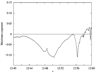
Figure 6. The largest Lyapunov exponents for A between 12)4 and 12)6.

The signs of the Lyapunov exponents provide a qualitative picture of a system dynamics. The criterion is

j'0 (chaotic) j)0 (regular motion).

The periodic and chaotic motions can be distinguished by the bifurcation diagram, while the quasiperiodic motion and chaotic motion may be confused. However, they can be distinguished by the Lyapunov exponent method. The Lyapunov exponents of the solutions of the non-linear dynamic system are plotted in Figure 6 as A"12)4 to 12)6.

There are a number of di!erent fractional-dimensional-like indices, e.g., the information dimensions, Lyapunov dimensions, and correlation exponent, etc., the di!erence between them is often small. The Lyapunov dimension is a measure of the complexity of the attractor. The introduction of Reference [8] the Lyapunov dimensions dL as

dL"j#+ji/1 ji_{D jj`1D} , (6.2) has been developed where j is de"ned by the condition

j +

i/1ji'0

and j`1+

i/1 ji(0.

The Lyapunov dimension for a strange attractor is a non-integer number. The Lyapunov dimension and the Lyapunov exponent of the non-linear system are listed in Table 1 for di!erent values of A.

TABLE1

¸yapunov exponents and ¸yapunov dimensions of the system for di+erent A

A j1 j2 j3 j4 + ji _dL 12)4 !0)0148 0 !0)1196 !5)4112 !5)5 1 Period-1 12)5 !0)1088 0 !0)1380 !5)2718 !5)5 1 Period-2 12)56 !0)0541 0 !0)1185 !5)2718 !5)5 1 Period-4 12)578 !0)0175 0 !0)1191 !5)3551 !5)5 1 Period-8 12)62 0)0613 0 !0)1194 !5)4064 !5)5 2)513 Chaos

7. GLOBAL ANALYSIS BY MODIFIED INTERPOLATED CELL MAPPING METHOD

A brief introduction of the modi"ed interpolated mapping method [9] is given as follows. Let a point mapping system be governed by

Xn`1"f (Xn), X3R3, (7.1)

where f : R3PR3 and n is an integer. The basic concept of the interpolated mapping method is to "nd the image Xn`1 by using an interpolation procedure instead of the system. For a three-dimensional system, the region of interest D is speci"ed by a Cartesian product [x1min, x1max]][x2min, x2max]][x3min, x3max], which is divided into N1]N2]N3 cells. The size of cell is hi"(x*max!x* min)/Nt, i"1, 2, 3. The "rst mappings of cells in the region of interest are constructed by numerical integration to serve as the reference mappings for the interpolation. The interpolated mapping of each cell is constructed within the mapping periods assigned, such as 30 periods. Through these mapping sequences, periodic attractors with periods of less than 30 are located by the criterion 10~5 cell size. If no periodic attractor is located, the 30th maping of each cell is assigned to the "rst mapping, and then iterated forward to construct the next iteration of 30 mappings. If periodic attractors are located and a cell leads to a periodic attractor within the criterion 10~2 cell size, the cell is considered in the basin of attraction of the attractor.

For a three-dimensional system, 3033 cells are studied by the modi"ed interpolated mapping method, where 303 is the number of the total cells divided in each dimension of the region of interest.

The last three equations of equation (4.1) with the values of parameters are considered as follows:

xR "y,

yR "0)5 sin(x) y2/(3!cos2 (x))#13)158 sin(x) cos(x)/(3!cos2(x)) !0)347z/(3!cos2(x))#0)579(x2!1) cos(x)y/(3!cos2(x)) !1)342A sin(x) cos(x) sin(1)1588q)/(3!cos2(x)),

zR "!78)95 sin(x)/(3!cos2 (x))!sin(x) cos(x)y2/(3!cos2(x)) !3)476(x2!1)y/(3!cos2(x))#0)695 cos(x)z/(3!cos2 (x)

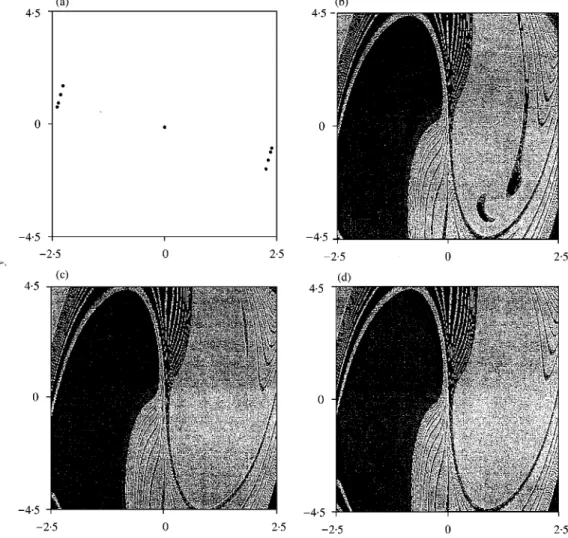
Figure 7. (a) The projection of attractors, (b) basins of attraction for z"0)1, (c) z"0)5, (d) z"1)0 for A"12)4.

where x is the angular co-ordinate of pendulum /, y is the angular velocity of pendulum/Q, and z is the velocity of block xRA.

Three black dots in Figure 7(a) for A"12)4 indicate that the system motion is period-1 motion and the corresponding basis of attraction are shown in Figure 7(b)}(d) with z"0)1, 0)5, 1)0 respectively. The symbols && ) '' and &&]'' denote the cells attracted by di!erent period-1 stable solutions respectively. For A"12)5, Figures 8(a)}8(d) show the phenomena of period-2 motion. For A"12)56, Figures 9(a)}9(d) show the phenomena of period-4 motion

8. CONTROLLING CHAOS

Several kinds of interesting non-linear dynamic behavior of the system were studied in the previous sections. They have shown that the forced system exhibited both regular and chaotic motion. Usually chaos is unwanted or undesirable.

Figure 8. (a) The projection of attractors, (b) basins of attraction for z"0)1, (c) z"0)5, (d) z"1)0. for A"12)5.

In order to improve the performance of a dynamic system or avoid the chaotic phenomena, we need to control a chaotic system to a periodic motion which is bene"cial for working with a particular condition. It is thus of great practical importance to develop suitable control methods. Very recently, much interest has been focused on this type of problem-controlling chaos [10}13]. For this purpose, the delayed feedback control, the addition of constant motor torque, the addition periodic force, and adaptive control algorithm (ACA) are used to control chaos. As a result, the chaotic system can be controlled.

8.1. CONTROLLING OF CHAOS BY DELAYED FEEDBACK CONTROL

Let us consider a dynamic system which can be simulated by ordinary di!erential equations. We imagine that the equations are unknowns, but some scalar variable

Figure 9. (a) The projection of attractors, (b) basins attraction for z"0)1, (c) z"0)5, (d) z"1)0, for

A"12)562.

can be measured as a system output. The idea of this method is that the di!erence D(t) between the delayed output signal y(t!q) and the output signal y(t) is used as a control signal. In other words, we use a perturbation of the form

F(t)"K [y(t!q)!y(t)]"KD(t). (8.1) Hereq is a delay time. Choose an appropriate weight K and q of the feedback and one can achieve the periodic state. If K"0)2, 0)04, 0)02 andq"2n/X, the results are shown in Figure 10.

This control is achieved by the use of the output signal, which is fed back into the system. The di!erence between the delayed output signal and the output signal itself is used as a control signal. Only a simple delay line is required for this feedback control. To achieve the periodic motion of the system, two parameters, namely, the time of delayq and the weight K of the feedback, should be adjusted.

Figure 10. (a) K"0)2, the period-1¹ motion of system after feedback control.

8.2. CONTROLLING OF CHAOS BY ADDITION OF A CONSTANT TORQUE

Interestingly, one can even add just a constant term to control or quench the chaotic attractor to a desired periodic one in a typical non-linear non-autonomous system. It ensures e!ective control in a very simple way. In order to understand this simple controlling approach in a better way, this method is applied to system (4.1) numerically.

In the absence of the constant motor torque, the system exhibits chaotic behavior under the parameter condition A"12)6.

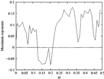
Consider the e!ect of the constant motor torque M added to the right-hand side of the last equation of equation (4.1). By increasing it from zero upwards, the chaotic behavior is then altered. Spectral analysis of the Lyapunov exponents has proven to be the most useful dynamical diagnostic tool for examining chaotic motions. In Figure 11, the maximal Lyapunov exponents are shown. It is clear that the system returns to regular motion, when the constant torque M is presented in certain intervals.

8.3. CONTROL OF CHAOS BY THE ADDITION OF PERIODIC FORCE

One can control system dynamics by the addition of external periodic force in the chaotic state. For our purpose, the added periodic force, b sin (u6t#/), added to the

Figure 10. (b) K"0)04, the period-2¹ motion of system after feedback control.

right-hand side of the last equation of equation (4.1), is given. The system can then be investigated by a numerical solution, with the remaining parameter "xed. One case is to examine the change in the dynamics of the system as a function of b for "xedu6"1)5, /"0. The maximal Lyapunov exponents are estimated numerically; the results are shown in Figure 12. At certain intervals, the maximal Lyapunov exponentsji)0, which indicates that the predictability of the system, recovers.

8.4. CONTROLLING CHAOS BY ADAPTIVE CONTROL ALGORITHM (ACA)

Recently, Huberman and Lumer [12] suggested a simple and e!ective adaptive control algorithm which utilizes an error signal proportional to the di!erence between the goal output and the actual output of the system. The error signal governs the change of parameters of the system, which readjusts so as to reduce the error to zero. This method can be explained brie#y: the system motion is set back to a desired state Xs by adding dynamics to the control parameter P through the evolution equation

PQ "eG(X!Xs), (8.2)

where the function G is proportional to the di!erence between Xs and the actual output X, ande indicates the sti!ness of the control. The function G could be either linear or non-linear. In order to convert the dynamics of system (4.1) from chaotic

Figure 10. (c) K"0)02, the period-4¹ motion of system after feedback control. motion to the desired periodic motion Xs, the chosen parameter A is perturbed as

AQ "e(X!XS). (8.3)

Ife"0)145, the system can reach the period-1 and period-2 as shown in Figures 13(a) and 13(b).

8.5. CONTROLLING CHAOS BY BANG-BANG CONTROL

Time-delay map is used in this control algorithm. Let

e(t)"X(t)!X(t!q) (8.4)

where q is the external torque frequency. De"ne <(t)"e(t)2 which is always positive or zero,

<Q "2 e(t) eR(t) _(8.5)

If <Q )0 then <(t)P0; e(t)P0 and X(t)PX(t!q).

By determining that equation (8.5) is less than or greater than zero, the control law can be determined. Assume

xR 1"F1(x1, x2, x3, x4, t), xR 2"F2(x1, x2, x3, x4, t),

Figure 11. The maximal Lyapunov exponents against M.

Figure 12. The maximal Lyapunov exponents against b withu"1)5, /"0.

xR 3"F3(x1, x2, x3, x4, t)#u,

xR 4"F4(x1, x2, x3, x4, t). (8.6)

IfE e(t) E)d, where d'0 is a present small value, u(t)"0. If E e(t) E'd then u(t)"!

G

K(F3 (x1, x2, x3, x4, t)!xR3(t!q)) when e(t)(0.

These results are similar to those in the case of an external force control and delayed feedback control. However, external perturbation or computation is

Figure 13. (a) The period-1¹ motion of system after adaptive control.

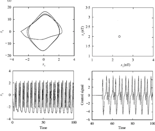
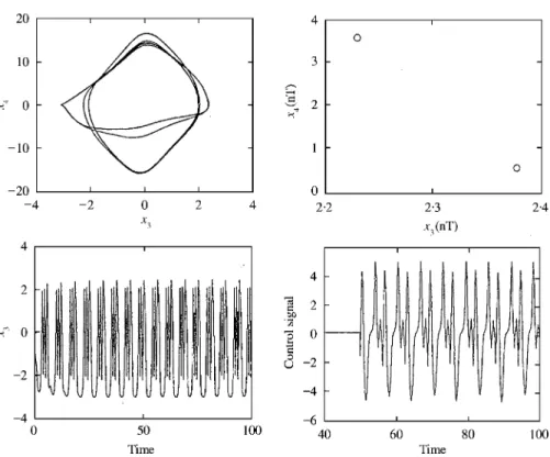
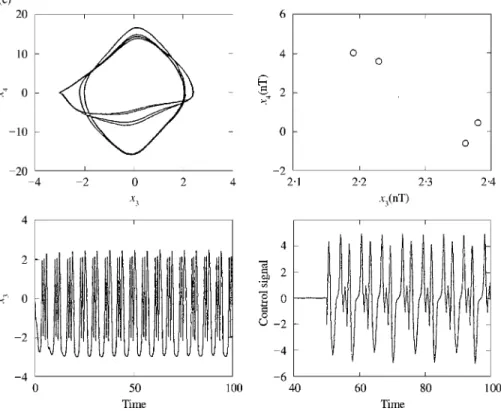
Figure 14. Bang-Bang control is used to control period-2 for K"0)02; (a) phase portrait before control, (b) steady state after control, (c) period-¹ map before control, (d) period-¹ map after control, (e) time history after control, (f ) control signal.

needed for this control. Figure 14(a) shows the phase diagram of the system before control, and Figure 14(b) shows the phase diagram after control and each period-¹ map is plotted in Figures 14(c) and 14(d). Figure 14(e) shows the state evolution in the (x3!t) plane. In Figure 14(f) we have plotted control signal as a function of time.

9. CONCLUSIONS

The dynamic system of the elliptical pendulum exhibits a rich variety of non-linear behavior as certain parameters vary. Due to the e!ect of non-linearity, regular or chaotic motions may occur. In this paper, both analytical and computational methods have been employed to study the dynamical behavior of the non-linear system.

The stability conditions for the system have been found by using the Lyapunov direct method.

The periodic, and chaotic motion of the non-autonomous system are obtained by numerical methods such as power spectrum, period-¹ map and Lyapunov exponents. Many non-linear and chaotic phenomena have been displayed in bifurcation diagrams. More information on the behavior of the periodic and the chaotic motion can be found in parametric diagrams. The changes of parameter play a major role in the non-linear system. Chaotic motion is the motion which has a sensitive dependence on initial condition in deterministic physical systems. The chaotic motion has been detected by using Lyapunov exponents and Lyapunov dimensions. Although the results of the computer simulation have some errors, the conclusions match the bifurcation diagrams. Besides, the global analysis of the non-linear system has been obtained by using modi"ed interpolated cell mapping (MICM).

The presence of chaotic behavior is generic for certain non-linearities, ranges of parameters and external force. Also, quenching of the chaos is presented, so as to improve the performance of a dynamical system. The delayed feedback control, the addition of constant motor torque, the addition of periodic force, adaptive control algorithm and Bang-Bang control are presented.

ACKNOWLEDGMENT

This research was supported by the National Science Council, Republic of China, under Grant Number NSC 83-0401-E-009-078. The authors thanks Dr. S.C. Lee for his enthusiastic help.

REFERENCES

1. F. C. MOON1992 Chaotic and Fractal Dynamics. New York: Wiley.

2. H. K. KHALIL1996 Nonlinear System. England Chi!s, NJ: Prentice-Hall.

3. R. W. BROCKETT 1982 Proceedings of IEEE 21st Conference on Decision and Control,

4. P. HOLMES 1983 Proceedings of IEEE 22nd Conference on Decision and Control,

365}370. Bifurcation and chaos in a simple feedback control system.

5. A. A. ZEVINand L. A. FILONENKO1988 Soviet Applied Mechanics 24, 821}825. Periodic

oscillation of a pendulum with horizontal vibration of the support point.

6. L. G. LOITZYANSKII and A. I. LUR'E 1948 A course in theoretical mechanics. Moscow:

National Publishing House of Techno-Theoretical Literatures, Forth edition. (in Russian); (Chinese Translation, Publishing House of Higher Education, Shanghai, 1956).

7. L. MEIROVITCH 1994 Method of Analytical Dynamics. Singapore: McGraw-Hill

Publishing Company.

8. P. FREDERICKSON, J. L. KAPLAN, E. D. YORKEand J. A. YORKE1983 Journal of Di+erental

Equations, 49, 185}207. The Liapunov dimension of strange attractors.

9. Z. M. GEand S. C. LEE1997 Journal of Sound and <ibration 199, 189}206. A modi"ed

interpolated cell mapping.

10. S. SINHA, R. RAMASWAMYand J. S. RAO1991 Physica D 43, 118}128. Adaptive control in

nonlinear dynamics.

11. Y. BRAIMAN and I. GOLDHIRSH 1991 Physical Review ¸etters 66, 2545}2548. Taming

chaotic dynamics with weak periodic perturbations.

12. E. OTT, C. GREBOGI and J. A. YORKE 1990 Physical Review ¸etters 64, 1196}1199.

Controlling Chaos.

13. B. A. HUBERMAN and LUMER 1990 IEEE ¹ransaction on Circuits and Systems 37,