Dynamic resource allocation for VBR video transmission

Dynamic Resource Allocation for VBR Video Transmission

Hsiu-Chi Yang and Hsueh-Ming Hang*

Dept. of Electronics Eng., National Chiao Tung University

1001 University Rd., Hsinchu 30050, TAIWAN, Republic of China

*Fax: 886-3-5723283, Email: hmhang©cc.nctu.edu.tw

ABSTRACT

The goal of this paper is to provide a feasible and flexible mechanism for variable bit rate (VBR) video transmission and to achieve high network utilization with statistical Quality of Service (QoS). In this paper, we employ a piece-wise constant rate smoothing algorithm to smooth the video coder outputs and propose a simple algorithm to determine the renegotiation schedule for the smoothed streams. In order to transmit video streams with renegotiation-based VBR service, we suggest a connection admission control (CAC) based on Chernoff bound using a simple yet quite accurate "binomial" traffic model. The experimental results show that our proposed method provides an easy and robust mechanism to support real-time video transmission in both homogeneous and heterogeneous connection environments.

Keywords: Quality of Services, Connection admission control, ATM, MPEG, VBR

1. INTRODUCTION

Variable bit rate (VBR) video coding, such as MPEG, plays an important role in providing high quality video for multimedia applications while maintaining a reasonable storage requirement and achieving high network utilization. But the highly bursty nature of the VBR compressed visual data makes network traffic management a very difficult task. For this reason, a number ofresearches have been conducted using video smoothing algorithms to reduce the bit rate variation in transmitting the compressed video from a server to a client across a high-speed network.1 These algorithms exploit client buffering capabilities and determine a smoothed rate transmission schedule, while ensuring neither overflow nor underfiow would appear at the client buffer.

The bit-rate statistical characteristics of a smoothed video are very different from the unsmoothed one. Therefore, we need different solutions to transmit the smoothed video streams. In this paper, we concentrate on proposing a scheme to transmit smoothed VBR videos. In order to achieve high utilization efficiency, simple but robust resource management and control mechanisms have to be employed. Thus we suggest a CAC algorithm based on Chernoff bound using a simple yet feasible traffic model requiring only three parameters and these parameters can easily be identified from video sources. Our experimental results indicate that our proposed CAC method based on the traffic model provides an easy and flexible mechanism to support real-time video transmission.

The rest of this paper is organized as follows. First, the characteristics of VBR MPEG videos in both the

unsmoothed and the smoothed cases are presented in Section 2. The mechanism for transmitting VBR MPEG video over ATM networks are addressed in Section 3. Section 4 contains various experiments that have been tested along with the evaluation of the efficiency of the proposed transmission scheme. Finally, Section 5 states our conclusions.

2. CHARACTERISTICS FOR VBR MPEG VIDEO

2. 1 .

MPEG

Bit-rate Characteristics and Characterization

Video applications have stringent requirements on QoS (cell loss rate, cell delay and etc.). To design the packet-switch networks that carry video signals, it is important to know the characteristics and to construct models accurately describing the bit-rate variation of video signals. More precisely, we like to predict: (1) the packet delay and loss due to statistical multiplexing, and (2) the buffer size and bandwidth required for carrying the multiplexed data. These two points are the keys to our CAC design.

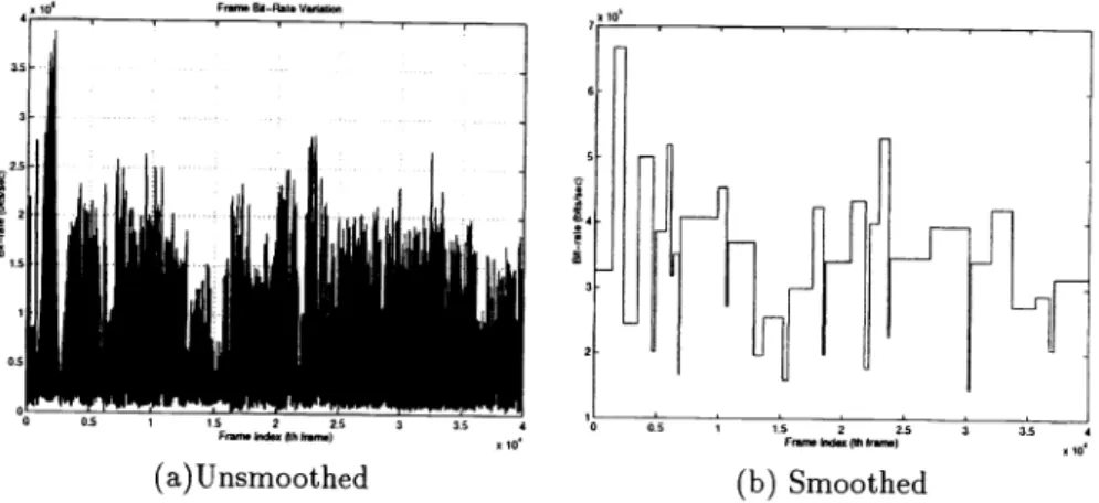
Figure 1(a) shows the frame bit rate variation of a VBR MPEG coded video, "Star Wars" 2 Thissequence

Figure 1. Bit-rate Variation of the compressed "Star Wars".

hL]

I

Figure 2. Impact of the Smoothing on Frame Bit Distribution.

365.6 Kbits/sec. As one can tell from Figure 1(a), the bit-rate variation can largely contribute to scene changes and the amount of motion within the scene.

Various video smoothing algorithms have be developed that utilize the client buffering capability to reduce the rate variation in the VBIt-compressed video. In this paper, we adopted a work-ahead smoothing technique which enables the server to achieve the largest possible reduction in rate variation when a stored video is transmitted to a client with a given buffer size.1 After being smoothed with this algorithm, the bit rate curve is nearly piece-wise constant. This means that cell arrival intervals are the same in a segment, and the short-term scale variations disappear (Figure 1(b)). The bit rate within a constant-rate segment is constant and the bit rate is almost random after smoothing. Figure 2 shows the histogram of the frame bit rate of "Star Wars" both for the unsmoothed case as well as the smoothed cases for client buffer sizes of 256 KBytes and 1 MBytes. This figure indicates that smoothing significantly reduces the range of transmission rate from 0-4.34 Mbits/sec in the unsmoothed schedule, down to 79-928 Kbits/sec for the 256 KByte client buffer, and 140-600 Kbits/sec for the 1 Mbyte client buffer. Note that the histogram of the smoothed case looks very different from that of unsmoothed one. Especially the long, heavy tail of the unsmoothed "Star Wars" trace is transformed into disconnected spikes after smoothing with the 1 Mbyte client buffer.

We can use Markov process to characterize the marginal distribution of the smoothed traces. However, it may need a number of parameters to match the model accurately. This is not practical for traffic management for high-speed networks. Many techniques have been suggested to characterize the smoothed video traces. In Section 3.5, we present a simple approach to characterize the marginal distribution of smoothed video streams. This approach is mainly designed for reducing the complexity in the CAC unit.

1.

hi

, I

(a)Unsmoothed (b) Smoothed

2.2. The Worst-case Model of ATM Traffic Descriptor

The ATM VBR connection service requires a traffic descriptor declared by the source at the connection set-up procedure. It consists three parameters: Peak Cell Rate (PCR), Substantial Cell Rate (5CR), and Maximum Burst Size (MBS). It is difficult to characterize VBR video traffics accurately by using only these three parameters. In this situation, CAC has to take the worst case into consideration. In Doshi,3 it is proposed that the full rate on-off source tends to be the worst case in the statistical multiplexing performance. For a given set of User Parameter Control (UPC) parameters (A,, , , Mb3), thelengths of on and off periods for a full rate on-off source are given by:

T0 =

_;s;t-

and T0 --

, respectively.

During the on periods, the source generates cells at the constant rate ), and is silent during the off periods. This model is quite popular; many researchers design CAC algorithms based on this model.46

3. TRANSMISSION SCHEDULE AND RENEGOTIATION-BASED SERVICE

As we have seen in Section 2, the bit-rate statistical characteristics of a smoothed video are very much different from the unsmoothed one. Therefore, we need different schemes in transmitting the unsmoothed and the smoothed video streams. We start with a discussion on an upper bound of the cell loss probability in a buffered multiplexer based

on the general Markovian source model.

3.1. Upper Bound on Cell Loss Probability

In ATM networks, the cell losses are often caused by buffer overflow at the multiplexers with finite buffer. In this section, we focus on the theoretical bound of the cell loss probability for a given Markovian source.

Let C and B denote, respectively, the link capacity and the output buffer size of a multiplexer, and Qbe the current queue in the output buffer. When Q

>

B, the next cells submitted to the network will be dropped.

Suppose there are K types of sources, and Nk sources of type k, 1 < k < K. At any time t 0, the rate of traffic

generation by source n of type k is rk(i). For each type k, we assume that rk(t) has a stationary distribution given by a Lk-state random variable rk, which

takes values {r, r r}, and Prob(rk =

_{rk))pk) Hence,}

. . _{K Nk}

the total amount of traffic at a random time is R :=

k1

_{n=1 rkn.}

Under the above assumptions, the stationary overflow probability can be approximated by 6:

F(B) =

P(Q

B) Lez13, when B is large

(1)

where L = _P(R> C) is the loss probability in bufferless multiplexing, which can be estimated from the Chernoff bound theorem and z is the dominant eigenvalue in the buffered multiplexers, which determines the large buffer behavior.

The Chernoff's theorem states that

log(P(R C)) _F*(s),

(2)

where

F*(s) =snp8<0F(s), (3)

F(s) =

sC

-

_{A(s), (4)}

A(s) =

_NklogM(s),

(5)

and Mk(5) =

fi

_pk)esrk) is the moment generating function of rk.

As C —+ccwith Nk/C =_0(1),k=1

P(R>C)c

(6)

where

2 *

ç'

M(s*)

M(s*) 2

The value s is the solution to F'(s) =C.

The dominant eigenvalue and its calculation have been topics studied extensively for statistical multiplexing based on stochastic fluid models. We refer the readers to Elwalid and Mitra7 for detail calculation and solutions of the dominant eigenvalue.

Based on the above approximations, we design a CAC scheme for heterogeneous video traffics. Inour experimental results, we can see that this scheme provides high network efficiency for video transmission.

3.2 . _{Renegotiation-based}

_{VBR Service}

The smoothed video output stream has piece-wise constant bit rate variations. For each constantrate segment, we have to renegotiate with the network to reserve a new service rate. In the renegotiation-based VBR service, a source can renegotiate its service rate by a call. A renegotiation process consists of sending a signaling_{message (for} example, FRP,8 RSVP9) requesting an increase or decrease of the current service rate. Upon successful completion of the signaling, the source is allowed to send data at the new rate. In addition, the network_{can monitor the traffic}

based on the renegotiated service rate. Because the bit-rate is constant during a segment, renegotiation-based service therefore retains the advantages of the simplicity and the small buffer sizes of the CBR services.

3.3. CAC Rule for Smoothed Videos

Because the bit-rate is constant in each segment (Figure 1(b)) of a smoothed video, insufficient bandwidth at_one point is like to lead to consecutive losses over a relatively long period of time when the buffer overflows. This leads to a significant decrease of the QoS for a client. Consequently, in supporting transmission of smoothed video streams with a guaranteed QoS, network bandwidth allocation becomes highly critical. If a CAC scheme is properly designed, the amount of buffer space needed within the network can be greatly reduced. For these_{reasons, we choose bufferless} Chernoff bound approximation discussed in Section 3.1 as our CAC rule.

Consider a bufferless multiplexer whose channel capacity is C. Suppose there are K types of sources same as described in Section 3.1. According to Eq. (6) we can estimate the aggregate bandwidth ê that is needed to satisfy a given loss probability bound e at the multiplexer; that is, P(R ê) < c. The estimated bandwidth is given by the following expression

(8) where .isthe solution to the following equation:

log(e) =_A(s)—

sA'(s)—log(s)—

_log(A"(s))

—

log(2)

. ₍₉₎

Based on this formula our CAC rule operates as follows.

CAC Rule

Suppose a new call of source type k arrives. It is accepted if the estimate bandwidth ()_{computedusing Eq. (8)} with Nk replaced by Nk + 1, is less than the given channel capacity C of a bufferless multiplexer.

The main cost of this CAC rule is the computation of the moment generating function Mk(5) and its first and second derivatives used in Eqs. (8) and (9). Clearly, using fewer parameters in capturing the traffic characteristics reduces the cost of CAC. Therefore, we focus on constructing a simple model to characterize smoothed video traces in the next two subsections.

3.4. Marginal Distribution Characterization

Because we adopt bufferless Chernoff-bound approach in designing our CAC rule, the difficult task of characterizing the correlation structure of the traffic is largely eliminated. Only the marginal distribution information is necessary in traffic specification. The stationary marginal distribution f(s) of a smoothed video v(t), t =1,2 ,Ncan be computed as follows:

f(s) =

:v(t) <x}I

_N

(10)

Before presenting a traffic model for CAC, we should note that the number of parameters in characterizing the source should be small and the loss probability estimated using the CAC rule should be an upper bound on the probability required by a source based on the given set of user-specified parameters, i.e., P(R C) < P(R C),

where R = >:<= >i::'

_rk,

and kn 5 a random variable representing the marginal distributionused by the CAC, which matches the user specified parameters. From Eq. (2), it suffices to show that e_F*(c) <e_F*().From Eq. (4) this is equivalent to

sup8o{sC — _A*(s)} —

A*(s)}, (11)

Clearly, P(R C) < P(R C) holds if A*(s) < A*(s)for all s 0.

3.5. Binomial Distribution Characterization for CAC

Although the Markov model with a number of states can achieve high accuracy in characterizing the marginal distribution of a single smoothed video stream; however, it is too complicated to be processed in real time in high-speed networking.

Perhaps the simplest way to characterize the marginal distribution of a video is to use a model with only two parameters: the peak rate, i, and the mean rate, in. Similar to the on-off model we discussed in Section 2.2, a random variable X ,_takingtwo values: X = 0 with probability 1 — and X with probability ,isthe worst

case with the same in and

The on-off model based only on the mean and peak rate of a source generally does not provide sufficient information about the marginal distribution of the source. Therefore it leads to a rather conservative loss probability estimate by the Chernoff bound. Thus we propose a simple "binomial" model to characterize the marginal distribution of a smoothed video below. In addition to the two parameters representing the mean in and the peak i, we introduce a third parameter, M, representing the step number of the the bit rate; i.e., the entire bit rate range is divided into M equidistant segments.

Given these three parameters, we use X with "binomial" distribution defined below to characterize the smoothed video streams for the purpose of CAC.

P(=kA)= (

)pk(i_p)M-k ,k=1, 2

,

M

(12) where .1

MA=,

MAp=rn,

or equivalently, —

Basedon these definitions, the modeling procedure is transformed to finding the feasible M for a given source. Note that the binomial distribution defined above probably cannot match Eq. (11) for all s 0, but we find that the value s is located in an interval [a, /3] when the loss probability is given in the scale of i0 in our experiments. We can use this property to search for the feasible M. From Eq. (6) and related formulas, we can see that the value of ? is determined by link capacity and the probability distribution of the video bit rates. Based on these observations, our searching process is described below.

Step 1:

Estimate the value of a and 3 by training with some videos in advance. In the training process we start with a given cell loss probability and the link capacity for data transmission. Then, define a benchmark which consists of various type of smoothed videos. At last, construct aggregate traffics randomly and increase the traffic load until the loss probability estimated by Eq. (6) achieves the scale we defined. Then record the s values, and find the bounding interval {c, 9].

Step 2:

:__

(a) Terminator (MPEG-i Movie) _{(b) ATP (MPEG-i Sport)}

(c) Talki (MPEG-i Talk Show) (d) Brother (MPEG-2 Movie)

Figure 3. Comparison of moment generation functions between the real and the binomial model distributions. Suppose Mk(S) is the moment generation function computed by the original bit rate distribution for a type k video, e.g., the values of r(c)andp(C) of the video. Then the M can be calculated by following expression

M=Max{M: (i—p)+pe'i Mk(L3)},

(13)

where p and are_{formulated by Eq. (12).}

Based on the benchmark video traces we used in experiments, we find that the s j located in the interval [1O_6, iO] which was obtained from the training process in Step 1. Using this interval at Step 2 of the searching process, we can find the value M for each trace. Figure 3 shows the results of this process. We can see that the moment generation functions of the binomial distribution we find match the original distribution well. Especially in Figure 3(d) ,we need to use log function to separate the two lines; otherwise, they overlap. We then conduct experiments to evaluate the performance of CAC with this method, which will be discussed in Section 4.

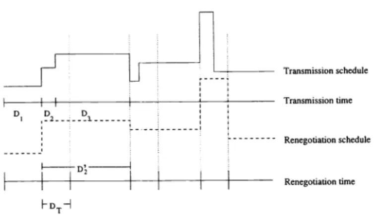
3.6. Renegotiation Schedule

Renegotiation-based service adds a bandwidth renegotiation mechanism to the static CBR or VBR service. In Salehi et al.' and Figure 1(b), we can see that the smoothing algorithm provides a transmission schedule for a video with a set of (R ,

_D)

, where R denotes the constant transmission rate over the segment with duration D2 ,i

=

1_, . . . , M,

where M is the segment number of the entire smoothed video. Therefore, it is reasonable to employ Renegotiated CBR (RCBR)4 service for our transmission schedule. In fact, the name "Renegotiation Based VBR service" we used in this paper should be interpreted as "VBR service implemented by employing RCBR".

Intuitively, we can renegotiate a new bandwidth reservation at the beginning of each segment. However, in our experiments, we find that a new renegotiation for each segment may be impractical. For example, the smoothed "Star

Transmission schedule

Transmission time

Renegotiation schedule

Renegotiation time

Figure 4. The concept of renegotiation schedule.

Wars" with a 256Kbyte buffer results in 174 segments and the lengths of some segments are as short as 900 ms. Take the packet round-trip time into consideration, it is useless to renegotiate a new bandwidth reservation if the length of the segment is shorter than the packet round-trip time. Before we receive a connection acknowledgment, we have to renegotiate another new reservation. Furthermore, we define a threshold DT to reduce the cost of renegotiation signaling overhead. Therefore, the transmission schedule and reservation schedule are not always identical during transmission.

Figure 4 shows the concept of reservation schedule based on the transmission schedule. Let (Ri, Di): i=1,. .. ,M denote the transmission schedule we obtain from the smoothing algorithm in1 and DT denote the threshold of the renegotiation time duration. After the connection is setup, the server starts to transport video data based on (R1, D1). When D1 is expired, the server has to renegotiate a new bandwidth based on R2. However, if D2 is smaller than DT the following process is applied.

D =

i=2

D where n = mint{ DT} ,

(14)

R=max{RIi2,...,n} where n=rnint{DT}.

(15)

However, some bandwidth is wasted in this situation. Intuitively, a larger DT leads to more wasted bandwidth. We can decide the optimal DT based on a network pricing function which indicates the cost to a given reservation schedule of the form:

.

p

= (c) + 7

, (16)

where N is the length of the session at frame level, c is the bandwidth reserved at time i, (x) is the cost of

reserving bandwidth x over one time interval, -y is the fixed renegotiation cost, and 5a,b 1 if a b; 0, otherwise. For simplicity, we set q(cj) = c2 and y = 0. As a result, DT is chosen near the packet round-trip time which is usually in the order of 102 ms.

3.7. The Complete Transmission Scheme

In summary, our scheme for VBR video transmission is outlined as follows.

1. Determine the transmission schedule of a smoothed video stream based on the smoothing algorithm we employ. 2. Decide the renegotiation schedule based on the determined transmission schedule and the limits of renegotiation

mechanism.

3. Characterize the transmission schedule behavior using the binomial distribution. F DTH

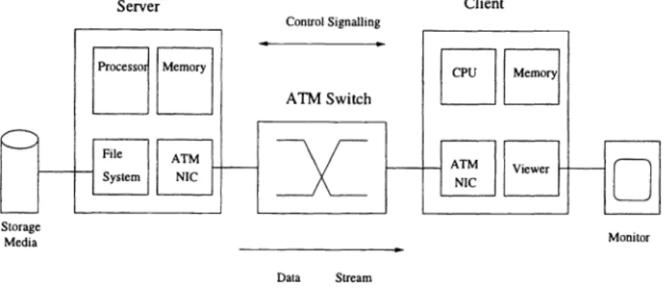
Server Client

Figure 5. A Simplified Video Transmission System.

4. Use the Chernoff bound CAC method to determine whether a connection request is admitted or denied based on the binomial model of transmission schedule selected in Step 2.

5. If the connection request is admitted, the video stream is transmitted according to the transmission schedule and the network resources are renegotiated according to the renegotiation schedule.

4. SIMULATIONS AND EXPERIMENTAL RESULTS

To study the behavior of MPEG traffic in an ATM network, we performed several simulation experiments using several MPEG traces and one MPEG-2 trace. In this section, the simulations and the experimental results are discussed. We start with a description of the simulation environment and the models of network as well as the end-systems used in the simulations. After describing the MPEG traces used in simulations, we continue to discuss the experimental results of the transmission schemes we proposed in Section 3.

4.1. Simulation Environment and Models

The simplified system considered in this study is shown in Figure 5. Because we focus on the efficiency of trans-mission schemes, the simple system should be sufficient for this purpose without loss of generality. It is obvious that the system is made of by three major components: servers, clients and connection network. In this section, we focus on the operations and models for each component.

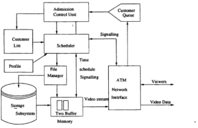
Consider the sever in Figure 6. To describe the cell streams produced by ATM adaptors in real situation, the following conditions are assumed.

1 .TheATM adaptor and the transmission link have the same capacity. 2. The ATM adaptor uses AAL type 5 to access the video data.

3. Two MPEG Transport Stream (TS) packets are included in one CPCSYDU.

This means that one AAL5SDU with size 376 (2x188) bytes will arrive at the ATM layer at the same time. Then the packetization takes place. After shaping, the conforming cells flow into the network and eventually reach the client buffer.

For clients (the viewers), the most important system design issue is to provide jitter-free playback. In our simulations, we assume that 128 Kbytes buffer is preallocated before playback and the total buffer size in a client system is 256 Kbytes. These two values affects the characteristics of cell streams smoothed by our smoothing algorithm. Therefore, the sever should negotiate these two values at the connection setup stage. Based on the negotiated values, the clients reserve the required buffer size and start to playback when enough data are loaded.

The cell loss probability is highly correlated with the output buffer size of a multiplexer. Large buffer size may reduce the loss probability, but it introduces long delay. There is a tradeoff between buffer size and delay. To achieve a reasonable delay, we assume that the buffer size of the multiplexer is in the order of i03 —

iO

in oui experiments.

Storage

Media - Monitor

Figure 6. The Server Architecture Diagram. Table 1. Encoder Parameters of MPEG-i Sequences

1 2

Encoder Input 384 x 288 pel

Color Format YUV (4:1:1, resolution of 8 bits) 3 Quantization Values 1=10, P=14, B=i8

4 Pattern IBBPBBPBBPBB

5 GOP Size 12

6 Motion Vector Search _{'Logarithmic' /}'Simple'

7 Reference Frame 'Original'

8 Slices 1

9 Motion Vector/Range half pel /10

10 Frame Rate 25 fps

4.2. Description of Traces

We use 15 MPEG-i traces and one MPEG-2 trace for simulations. All the MPEG-i traces we used are publicly available from anonymous the ftp sites.2'10 The MPEG-2 data is provide by A. Reidman of AT&T Research Labs.'1

The MPEG-i traces are extracted from sequences which have been encoded by the Berkeley MPEG-encoder

(version1.3), the encoding parameters for these sequences are listed in Table 1. Each MPEG video consists of 40,000

frames which is equivalent to approximately half an hour video. We also use a MPEG-2 trace in our simulations to show the system robust. The encoding parameters and characteristics of this trace are listed in Table 2.

4.3. Simulation Results

4.3.1. Binomial model matching

The objective of this experiment is to compute the parameters in our "binomial" model for smoothed video sources. For the given cell loss probability i0 and link capacity 155.52 Mbits/sec, the results of training process which is stated in Section 3.5 are listed in Table 3.

We can see that the value of ? is bounded in the interval [iO_6, i0] as in our test benchmark traces. Item ii is an aggregated cell stream composed of several different traces. It is included here to show that the estimated interval is suitable for both homogeneous and heterogeneous cases.

Using Step 2 of the matching process, we can estimate a feasible step number M for each trace. The results are shown in Table 4.

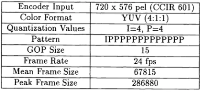
Table 2. Parameters of MPEG-2 Traces Encoder Input 720 x 576 pel (CCIR 601)

Color Format YUV (4:1:1) Quantization Values 1=4, P=4

Pattern IPPPPPPPPPPPPP

GOP Size 15

Frame Rate _{24 fps}

Mean Frame Size 67815

Peak Frame Size 286880

Table 3. The Values of s forOur Benchmark

iii

Training Source

Value of?

bond (MPEG-I movie) 2.26 x 10_6

—-- lambs (MPEG-I movie) 2.46 x 10_6 —--- star (MPEG-I movie)

2.61 x 10

—-— terminator (MPEG-I movie) 7.30 x 10_6

—— preview (MPEG-I movie)

3.09 x 10

—— ATP (MPEG-I sport)ATP

2.66 x 10

race (MPEG-I sport) 2.23 x 10_6

_!_ sbowl (MPEG-I sport) 2.84 x 10_6 soccer_i (MPEG-I sport) 2.64 x 10_6 soccer_2 (MPEG-I sport) 1.82 x 10_6

JL

mixed (MPEG-I + MPEG-Il)

2.ii x 10

Table 4. The Values of M for Traces

ii

Trace name

Value of M

bond (MPEG-I movie) 5

—__ lambs (MPEG-I movie) 5

star (MPEG-I movie) 5 —--_ terminator (MPEG-I movie) 9

—--- preview (MPEG-I movie) 6

----

ATP (MPEG-I sport) 8 race (MPEG-I sport) 7

—--- sbowl (MPEG-I sport) 10

—p--- soccer_i (MPEG-I sport) 8

Figure 8. Comparison of M values for the smoothed "ATP".

4.3.2. Performance evaluation of CAC rules

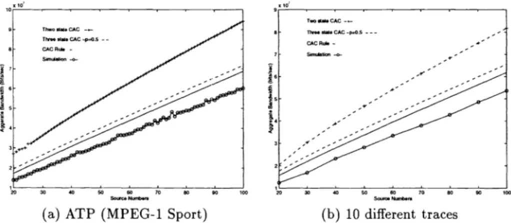
After identifying the parameters of the binomial model of the original source, we estimate the aggregated bandwidth needed for the current connection using Eq. (8). Figure 7(a) shows the performance for the smoothed "ATP" video, and Figure 7(b) shows the performance for 10 different smoothed traces simultaneously existing in the network. Five hundred independent runs are performed to obtain the minimum bandwidth needed to satisfy the given QoS requirement. We also compare our results with the CAC methods which employ a "two-state model" and a "three-state model" used in Zhang et al.5

The values of M we found in 4.3.1 is based on the goal of highest efficiency. In fact, we can balance the robustness of a network service and the amount of statistical multiplexing gain by altering the value of M ._Figure8 shows the estimated bandwidth with different value of M . Byreducing the value of M ,thebandwidth can be conservatively estimated to provide more robust services. In other words, a video can be transmitted at different level of QoS by selecting different M value.

We also find that the required bandwidth needed by smoothed video is significantly smaller than that needed by the unsmoothed video. The critical requirement of the buffer space in transmitting unsmoothed video at peak frames disappears after smoothing. On the other hand, the bit rate is constant during a long interval in the smoothed videos. Hence, if a renegotiation fails, the QoS may be damaged badly. Therefore, we need an extra process for handling renegotiation failures. For stored video, scalable coding method may be used for this purpose. For real-time on-line applications such as videoconferencing, the joint channel and encoder rate control may be a solution for renegotiation failures. These two techniques may become interesting topics for future researches.

(a) ATP (MPEG-i Sport) (b) 10 different traces Figure 7. Comparison of CAC rules for the smoothed videos.

5. CONCLUSIONS

In this paper, we have studied the problem of real-time video transmission from a server to a client across a high-speed network. Our study starts with characterizing videos in the different cases of smoothed and unsmoothed data streams. In particular, we find that two advantages are associated with video data smoothing. First, queuing delay jitter introduced by buffering within the network is greatly reduced because the bit rate is constant in each segment. In other words, the delay jitter is reduced by smoothing with a specified client buffer. Second, bandwidth allocation becomes nearly the only critical issue. Hence, we can neglect the effect of the buffer in analysis and only the marginal distribution information is needed in traffic specification for CAC. Therefore, we come up with a scheme for the smoothed video transmission with renegotiation based VBR service. Our experiments show that our scheme achieves better performance than the unsmoothed case and that our proposed CAC rule is robust in the heterogeneous cases. The renegotiation based services still have many open questions. A number of issues remain to be explored in the future.

REFERENCES

1. J. Salehi, Z. -L. Zhang, J. Kurose and D. Towsley, "Supporting Stored Video: Reducing Rate Variable and End-to-End Resource Requirements through Optimal Smoothing," ACM SIGMETRICS, Philadelphia, PA, May

1996.

2. ftp://ftp.bellcore.com/pub/vbr.video.trace/readme.html

3. B. T. Doshi, "Deterministic rule base traffic descriptors for Broadband ISDN: Worst case behavior and connection acceptance control," IEEE GlobeCom'93, pp.1759-1764, Dec 1993.

4. M. Grossglauser, S. Keshav and D. Tse, "RCRB: A Simple and Efficient Service for Multiple Time-Scale Traffic," IEEE/ACM Trans. on Neiworking, December 1997.

5. Z. -L. Zhang, J. Kurose, J. Salehi and D. Towsley, "Smoothing, Statistica' Multiplexing and Call Admission Control for Stored Video," IEEE Journal on Selecled Areas in Comm., vol. 15, no. 6, pp. 1148—1166, Augus

1997.

6. A. Elwalid, D. Heyman and T. V. Lakshman, "Foundamental Bounds and Approximationsfor ATM Multiplexers with Applications to Video Teleconferencing," IEEE Journal on Selecled Areas in Comm., vol. 13, no. 6, pp. 1004-1016,August 1995.

7. A. I. Elwalid and D. Mitra, "Effective Bandwidth of General Markovian Traffic Sources and Admission Control

of High Speed Networks," IEEE/ACM Trans. Networking. vol. 1, no. 3, pp.329-3'43, 1993.

8. P. Boyer and D. Tranchier, "A Reservation Principle with Application to the ATM Traffic Control," Computer Neiworks and ISDN Systems, vol. 24, pp. 321—334, 1992.

9. R. Braden, L. Zhang, S. Berson, S. Herzog and S. Jamin, "Resource ReSerVation Protocol (RSVP) —Version1 Functional specification" ,InternetEngineering Task Force, August 12, 1996

10. 0. Rose, "Statistical Properties of MPEG Video and Their Impact on Traffic Modeling in ATM System," Proceedings of the 20th Annual Conference on Local Computer Networks, Minneapolis, MN, 1995, pp. 397-406. Many MPEG-i traces are available via FTP from ftp://ftpinfo3.informatik.uni-wuerZburg.de /pub/MPEG/ ii. Private Communications.