First-principles theory of fluctuations in vortex liquids and solids
Baruch RosensteinNational Center for Theoretical Studies and Electrophysics Department, National Chiao Tung University, Hsinchu, Taiwan, Republic of China
共Received 19 February 1999兲
Consistent perturbation theory for thermodynamical quantities in type-II superconductors in magnetic field at low temperatures is developed. It is complementary to the existing expansion valid at high temperatures. Magnetization and specific heat are calculated to two-loop order and compare well to existing Monte Carlo simulations and experiments.关S0163-1829共99兲01829-9兴
Thermal fluctuations play much larger role in high-Tc
su-perconductors than in the low-temperature ones because the Ginzburg parameter G characterizing fluctuations is much larger. In the presence of magnetic field the importance of fluctuations in high-Tc superconductors is further enhanced.
A strong magnetic field effectively suppresses long-wavelength fluctuations in a direction perpendicular to the field reducing dimensionality of the fluctuations by two.1 Un-der these circumstances, fluctuations influence various physi-cal properties and even lead to new observable qualitative phenomena like vortex lattice melting into vortex liquid far below the mean-field phase transition line. It is quite straightforward to systematically account for the fluctuations effect on magnetization, specific heat or conductivity pertur-batively above the mean-field transition line using the Ginzburg-Landau 共GL兲 description.2 However, it proved to be extremely difficult to develop a quantitative theory in the interesting region below this line, even neglecting fluctuation of the magnetic field and within the lowest-Landau-level 共LLL兲 approximation.
To approach the region below the mean-field transition line T⬍Tmf(H) Thouless
3
proposed a perturbative approach around homogeneous 共liquid兲 state was in which all the ‘‘bubble’’ diagrams are resumed. The series provides accu-rate results at high temperatures, but for LLL dimensionless temperature aT⬅关T⫺Tmf(H)兴/(TH)2/3ⱗ⫺2 become
inap-plicable 共see dotted lines in Figs. 2 and 3 which represent successive approximants兲. Generally, attempts to extend the theory to lower temperature by Pade´ extrapolation were not successful and require additional external information about the low temperatures.6Alternative, a more direct approach to low-temperature fluctuation physics might have been to start from the Abrokosov solution at zero temperature and then take into account perturbatively deviations from this inhomo-geneous solution. Experimentally it is reasonable since, for example, specific heat at low temperatures is a smooth func-tion and the fluctuafunc-tions contribufunc-tion experimentally is quite small. This contrasts sharply with theoretical expectations.
A long time ago Eilenberger calculated the spectrum of harmonic excitations of the triangular vortex lattice.4 Subse-quently Maki and Takayama5noted that the gapless mode is softer than the usual Goldstone mode expected as a result of spontaneous breaking of translational invariance. The propa-gator for the ‘‘phase’’ excitations behaves as 1/关kz2⫹c(kx4 ⫹ky
4)兴. The influence of this unexpected additional
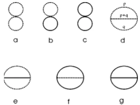
‘‘soft-ness’’ apparently goes even beyond enhancement of the con-tribution of fluctuations at leading order. It leads to disas-trous infrared divergences at higher orders rendering the perturbation theory around the vortex state doubtful. For ex-ample, contributions to energy depicted in Figs. 1共a兲 and 1共d兲 are, respectively, log2(L) and L4 divergent 共L being an IR cutoff兲 and at higher orders divergences get worse. Also qualitatively one argues7 共in a way similar to that used fre-quently to understand the Mermin-Wagner theorem8兲 that lower critical dimensionality for melting of the Abrikosov lattice is D⫽3 and consequently a vortex lattice in clean materials exists in the thermodynamic limit only at T⫽0. One therefore tends to think that nonperturbative effects are so important that such a perturbation theory should be abandoned9and it was abandoned. However, a closer look at diagrams like Fig. 1共d兲 共see some details below兲 reveals that in fact one encounters actually only logarithmic divergences. This makes the divergences similar to so-called ‘‘spurious’’ divergences in the theory of critical phenomena with broken continuous symmetry. In that case one can prove10 that they exactly cancel at each order provided we are calculating a symmetric quantity.
In this paper I show that all the IR divergences in free energy or other quantities invariant under translations cancel to the two-loop order. I calculate magnetization and specific heat to this order, interpolate with existing high-temperature expansion, and compare with Monte Carlo 共MC兲 simulation11 of the same system and experiments. Qualita-tively physics of a fluctuating D⫽3 GL model in the mag-netic field turns out to be similar to that of spin systems共or scalar fields兲 in D⫽2 possessing a continuous symmetry. In particular, although within perturbation theory in the thermo-dynamic limit the ordered phase 共solid兲 exists only at T⫽0, at low temperatures liquid differs very little in most aspects from solid. One can effectively use properly modified pertur-bation theory to quantitatively study various properties of the vortex-liquid phase.
The GL free energy is
G⫽ ប 2 2mab
冏
冉
ⵜជ⫺ ie* c Aជ冊
冏
2 ⫹ ប 2 2mc兩z兩 2⫹a兩兩2⫹b 2兩兩 4. 共1兲 Here Aជ⫽(⫺By,0) describes a nonfluctuating almost con-stant magnetic field in the c direction. Within the LLLap-PHYSICAL REVIEW B VOLUME 60, NUMBER 6 1 AUGUST 1999-II
PRB 60
proximation can be expanded in a basis of quasimomen-tum k eigenfunctions 共x兲⫽v共x兲⫹21
冕
d2kk共x兲冑
␥k 2兩␥k兩 共 Ok⫹iAk兲, 共2兲 k⫽冑
2冑
a⌬l⫽⫺⬁兺
⬁ exp再
i冋
l共l⫺1兲 2 ⫹ 2 a⌬l共x⫺ky兲⫺xkx册
⫺1 2冉
y⫹kx⫺ 2 a⌬l冊
2冎
.The unit of length will be the magnetic length lH ⬅
冑
cប/eH and a⌬⬅冑
4/) is the lattice spacing. The k ⫽0 component 0(x)⬅(x) is ‘‘a vacuum’’ with itsvacuum expectation value denoted by v. The integration is
over the Brillouin zone. Instead of one complex field two real fields O and A were introduced. They are somewhat analogous to acoustic and optical phonons in the usual solids with some peculiarities due to the strong magnetic field studied in detail by Moore.6 For example, the A mode corresponds to shear of the two-dimensional lattice. Substi-tuting Eq. 共2兲 into the free energy, quadratic terms in fields define propagators, while cubic and quartic are interactions. The phase factors containing a function ␥k
⬅兰x*(x)*(x)k(x)⫺k(x) are introduced in order
to diagonalize the resulting quadratic part PO⫺1(k)Ok*Ok ⫹PA⫺1(k)Ak*Ak, where PO,A⫺1(k,kz)⫽2a⫹2bv2(2k
⫾兩␥k兩)⫹kz
2 共to simplify intermediate expressions an
isotro-pic case mab⫽mc is considered, results are generalized
later兲. Functions ␥k⫽(⫺k,k) and k
⬅兰x*(x)(x)k*(x)k(x)⫽(0,k) as well as all the
three- and four-leg vertices can be expressed via a single function of two quasimomenta
共k1,k2兲⫽
兺
l,m 共⫺兲 lmexp再
i2 a⌬关lk1 y⫹mk 2 y兴 ⫺1 2冋冉
k2 x⫺2 a⌬l冊
2 ⫹冉
k1x⫺2 a⌬m冊
2册冎
. 共3兲 For example, the Ak1Ak2A⫺k1⫺k2 vertex isibv Re关共k1,k2兲兴⫽ ibv 2 02 A共k 1 x k1y⫹k2xk2y兲⫹O共k4兲, 共4兲 where stA⬅(2/a⌬)4兺l,mlsmt(⫺)lmexp兵⫺ 关(2)2/2a⌬
2
兴 (l2
⫹m)2其. If the fluctuations were absent the expectation value v0
2⫽a/
Ab would minimize G0⫽⫺av2⫹ (b/2)Av4where
A⬅00
A⫽1.16. The propagators entering Feynman
dia-grams, therefore, are
PO,A共k兲⫽ 1 MO,A2 共k兲⫹kz2; MO,A2 共k兲⬅2a A共⫺A ⫹2k⫾␥k兲. 共5兲
Expanding around k⫽0 using explicit expressions for ␥k
andkone observes that the constant and the k2 terms
van-ish, so that the 共only兲 leading quartic term is MA2(k) ⫽ (22
A
/2A)兩k兩4.
At the one-loop level the fluctuation contribution to the free energy is G1⫽ 1 2 1 共2兲3/2
冕
kz冕
k兵 ln关PO共k兲兴⫹ln关PA共k兲兴其. 共6兲One should minimize G0⫹G1 with respect to v leading to
the correction to its value
v1 2⫽ 1 共2兲3/2
冕
kz冕
k关PO共k兲⫹PA共k兲兴 ⫽2共21兲1/2冕
k冋
1 MO共k兲⫹ 1 MA共k兲册
. 共7兲Due to the additional softness of the A mode the second ‘‘bubble’’ integral diverges logarithmically in the infrared. This means that for the infinite cutoff fluctuations destroy the inhomogeneous ground state, namely the state with lowest energy is a homogeneous liquid.13 Since the divergence is logarithmic we are at lower critical dimensionality in which an analog of the Mermin-Wagner theorem8is applicable. It, does however, not necessarily mean that perturbation theory starting from the ordered ground state is inapplicable. The way to proceed in these situations have been found while considering simpler models like the 4 model F⫽1
2(ⵜi)2
⫹V(i 2
) in D⫽2 with a number of components larger then 1, say i⫽1,2.12 Considering the statistical sum, one first in-tegrates exactly zero modes existing due to continuous sym-metry 共translations in our case兲 and then develops a pertur-bation theory via the steepest descent method for the rest of the variables. When the zero mode is taken out, a single configuration appears with the lowest energy and the steepest descent is well defined. For invariant quantities such as en-ergy, this procedure simplifies to: one actually can forget for a moment about integration over the zero mode and proceed with the calculation as if it is done in the ordered phase. The invariance of the quantities ensures that the zero-mode inte-gration trivially factorizes. This is no longer true for nonin-variant quantities for which the machinery of ‘‘collective co-ordinates method’’ should be used.14
To the two-loop order one gets several classes of dia-grams, see Fig. 1. The leading-order propagators are denoted by dashed and solid lines for the ‘‘supersoft’’ A and ‘‘hard’’
FIG. 1. Contributions to the free energy at the two-loop level.
B modes, respectively. The共naively兲 most divergent diagram Fig. 1共d兲 actually converges. To see this one writes explicitly its expression in terms of the function
b2v2 2共2兲3/2
冕
q冕
p ID共q,p兲PA共p兲PA共q兲PA共p⫹q兲; 共8兲 ID共q,p兲⬅⫺共p,⫺q兲共p,q兲⫹4共p⫹q,p兲共p⫹q,q兲 ⫻ ␥p⫹q 兩␥p⫹q兩 ⫺ 2共p⫹q,⫺q兲共p,⫺q兲 ␥p␥p*⫹q 兩␥p␥p⫹q兩 ⫹2共q,⫺p兲2 ␥p␥q␥p*⫹q 兩␥p␥q␥p⫹q兩 ⫹ c.c.The integrals over pz and qz can be explicitly performed
using a formula 1 2
冕
p冕
q 1 p2⫹M12 1 q2⫹M22 1 共p⫹q兲2⫹M 3 2 ⫽ 2 1 M1M2M3 1 M1⫹M2⫹M3 .The leading divergence
⬃
冕
p冕
q Ia共q,p兲 1 p2q2兩q⫹p兩2 1 p2⫹q2⫹兩q⫹p兩2, is determined by the asymptotics of ID(q,p) as both p and qapproach zero. If ID⬃1, it would diverge as L4. However,
the vertex is ‘‘supersoft’’ at small quasimomenta ⬃p2 ac-cording to Eq. 共4兲, so that the expansion of ID(q,p) starts
from terms quartic in p and q and there is no singularity at the origin. This goes beyond the usual ‘‘softness’’ of inter-actions of the Goldstone modes (⬃p). Nonleading diver-gences can be found by analyzing contributions coming from three regions on which one of the line momenta p, q or p ⫹q vanishes. The corresponding expressions are
⬃
冕
k冕
l IDi共l兲 1 k2MA共l兲3 , with ID1⫽0, ID2⫽2l⫺l兩␥l兩 and ID 3⫽⫺ l 2⫹ l兩␥l兩,respec-tively. Here k denotes an IR divergent momentum while in-tegration over l is nonsingular. Although the second and the third contributions are divergent their sum is convergent.
Standard methods similar to the one used above can be applied to evaluate IR divergences of other superficially less divergent diagrams. There are no power divergences—only log2L and log L. The results are
b &
冕
p 1 MA共p兲冕
q冋
A⫺兩␥q兩 MA共q兲 ⫹ 兩␥q兩 MO共q兲册
, b &2冕
p 1 MA共p兲冕
q 2q⫹兩␥q兩⫺3A MA共q兲 , b &2冕
p 1 MA共p兲冕
q 2k⫺兩␥q兩 MO共q兲for Figs. 1共a兲, 1共b兲, and 1共e兲, respectively. In addition to direct contributions from G2 共Fig. 1兲, there is also a
‘‘cor-rection term’’ due to the cor‘‘cor-rection in the value of v from
Eq. 共7兲 inserted into the lower order contributions to free energy G0 and G1. Its divergent part is
⫺ b &2
冕
p 1 MA共p兲冕
qជ冋
2k⫺兩␥q兩⫺A MA共q兲 ⫺ 2k⫹兩␥q兩 MO共q兲册
.Both the leading divergences log2L and the next-to-leading ones log L cancel between the four contributions. Similar cancellations of all the logarithmic IR divergences occur in scalar models with Goldstone bosons in D⫽2 and D⫽3 共where the divergences are known as ‘‘spurious’’兲.
The finite result for the Gibbs free energy to two loops 共finite parts of the integrals were calculated numerically兲 is restoring the original units and reintroducing the asymmetry mc⫽mab: G⫽ ប 2 eHkBT
冑
mab g; g⫽⫺ 1 2A aT2⫹c1冑
兩aT兩⫹c2 1 兩aT兩 , 共9兲 where numerical values of the coefficients are c1⫽3.16 andc2⫽7.5. The dimensionless entropy 共LLL scaled
magnetiza-tion兲 s⫽⫺ dg daT ⫽
冉
2c5m ab 3 b 8e5k B 2m c冊
1/3 M 共TH兲2/3 ⫽1 A aT⫹ c1 2 1 兩aT兩 ⫺ c2 1 aT2, 共10兲and specific heat normalized to the mean-field value
1 A C ⌬C ⫽⫺ d2g daT 2⫽1⫹ c1 4 1 兩aT兩3/2 ⫹2c2 1 aT 3, 共11兲
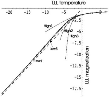
for successive partial sums are plotted in Figs. 2 and 3 共dashed lines兲. Qualitatively they are in accord with numer-ous experiments and MC simulations.11 At low temperature magnetization is a bit larger than that of the mean field, while dimensionless specific heat characteristically grows before dropping fast around aT⫽⫺5. To make a more
de-tailed comparison, I interpolated between the results of low-temperature expansion and those of high-low-temperature expan-sion using the following rational form for the free energy in terms of the often-used variable x defined implicitly by x ⫽y2, a
T⫽4(2y)2/3(1⫺1/8y2):
g⫽4共2y兲2/31⫹a1y⫹¯⫹an⫹2y
n⫹2
1⫹b1y⫹¯⫹bnyn
. 共12兲
The coefficients were constrained from both the low- and high-temperature sides. It has been already noted6that con-straining from both sides the Pade´ approximants, just by the first term at low energy, improves otherwise unsatisfactory magnetization and specific heat.
Adding two more terms on the low-temperature end makes it very close to the MC results 共stars triangles, and diamonds correspond to the 1, 2, and 5 T results for Y-Ba-Cu-O兲. I used just three leading terms in the
temperature expansion shown in Figs. 2 and 3 by the dotted lines. Using more terms does not modify significantly the result. Although magnetization curve Eq. 共12兲 agrees with that of Ref. 15, the specific heat is not.
To summarize, it is established up to the order of two loops that perturbation theory around the Abrikosov lattice is consistent. All the IR divergences cancel due to soft interac-tions of the soft mode. Perturbative results as well as inter-polation with the high-temperature expansion agree very well with the direct MC simulation.
Now I comment on the range of validity of the perturba-tive results and nonperturbaperturba-tive effects. As can be seen from Figs. 2 and 3, the range of validity of the low-temperature expansion presented in this paper is below aT⫽⫺10, while
that of the high-temperature expansion is above aT⫽⫺2.
Both exclude the range in which a small magnetization jump
共not seen in the scale of Fig. 2兲 due to vortex melting is seen experimentally and in the numerical simulation. Since the MC simulation is the only systematic tool available in the intermediate region关the theory of Tesˇanovic´ et al.15captures the major 共98%兲 contribution, but does not treat the small 共2%兲 effect including melting兴, one might have two possibili-ties to discuss such a singularity within the present frame-work. One possibility is that the jump is due to finite-size effects and disappears in the thermodynamic limit 共value of the cutoff in the simulation is only L⬃25兲. Another is that some nonperturbative effects can stabilize the vortex lattice. Quantitative comparison with experiments on Y-Ba-Cu-O was attempted in Refs. 11 and 15. The present simple inter-polation formula Eq.共12兲 works equally well.
The author is very grateful to L. Bulaevsky for encour-agement and numerous discussions, R. Sasik for providing the original MC data, and explaining the details of his MC simulation, Y. Kluger and other members of T11 and T8, especially A. Balatsky for discussions and hospitality in Los Alamos where part of this work was done. The work was supported by a grant from the NSC of Taiwan.
1
E. Brezin, D. R. Nelson, and A. Thiaville, Phys. Rev. B 31, 7124 共1985兲.
2M. Tinkham, Introduction to Superconductivity 共McGraw-Hill,
New York, 1996兲.
3D. J. Thouless, Phys. Rev. Lett. 34, 946共1975兲; G. I. Ruggeri and
D. J. Thouless, J. Phys. F 6, 2063共1976兲; S. Hikami, A. Fujita, and A. I. Larkin, Phys. Rev. B 44, 10 400共1991兲.
4G. Eilenberger, Phys. Rev. 164, 628共1967兲.
5K. Maki and H. Takayama, Prog. Theor. Phys. 46, 1651共1971兲. 6G. J. Ruggeri, J. Phys. F 9, 1861共1979兲; M. A. Moore, Phys. Rev.
B 41, 7124共1996兲.
7M. A. Moore, Phys. Rev. B 39, 136共1989兲; 45, 7336 共1992兲; 55,
14 136共1997兲.
8
N. D. Mermin and H. Wagner, Phys. Rev. Lett. 17, 1133共1966兲.
9G. J. Ruggeri, Phys. Rev. B 20, 3626共1978兲. 10F. David, Commun. Math. Phys. 81, 149共1981兲.
11R. Sasik and D. Stroud, Phys. Rev. Lett. 75, 2582共1995兲. 12A. Jevicki, Phys. Lett. 71B, 327共1977兲.
13Note that this共gauge-invariant兲 argument is completely
indepen-dent of choice of the ‘‘order parameter’’ or ‘‘gauge-invariant phase’’; see Ref. 7, and references therein.
14R. Rajaraman, Solitons and Instantons共North-Holland,
Amster-dam, 1982兲.
15Z. Tesˇanovic´ et al., Phys. Rev. Lett. 69, 3563 共1992兲; Z.
Te-sˇanovic´ and A. V. Andreev, Phys. Rev. B 49, 4064共1994兲; S. W. Pierson et al., ibid. 57, 8622共1998兲.
FIG. 2. Scaled magnetization defined in Eq.共10兲. Dashed 共dot-ted兲 lines are successive low- 共high-兲 temperature approximants, while the solid line is the interpolation. The points are the MC results.
FIG. 3. Scaled specific heat defined in Eq.共11兲. The same no-tations as in Fig. 2.