Optimal detection of solitons with timing jitter
Keang-Po HoInstitute of Communications Engineering and Department of Electrical Engineering, National Taiwan University, Taipei 106, Taiwan
Received November 29, 2004; revised manuscript received April 14, 2005; accepted April 23, 2005 When a soliton signal is detected by the maximum-likelihood principle, other than walk-out of the bit interval, timing jitter does not degrade the performance of the receiver. When the maximum-likelihood detector (MLD) is simulated by using the importance sampling method, even with a timing-jitter standard deviation the same as the full width at half-maximum of the soliton, the signal-to-noise (SNR) penalty is just about 0.2 dB. The MLD performs far better than the conventional scheme to lengthen the decision window with SNR degradation proportional to the increase of the window width. © 2005 Optical Society of America
OCIS codes: 060.5530, 190.5530, 060.4370.
1. INTRODUCTION
The Gordon–Haus timing jitter1 limits the transmission distance of a soliton communication system. Without any in-line control, the arrival time of the soliton has a vari-ance increasing cubically with the transmission distvari-ance. Although timing jitter can be reduced using an in-line filter,2,3 an in-line modulator,4 or other methods,5 it re-mains one of the major limitations for soliton transmis-sion systems. For a system with in-line timing-jitter con-trol, the transmission distance can be extended to long distances.4,6 When amplifier noise is accumulated with the transmission distance, the signal-to-noise ratio (SNR) reduces for the extended distance, and the optical ampli-fier noise becomes the primary limitation of the system.
Instead of another method among many methods5 to reduce timing jitter in the fiber link, this paper discusses a method to detect the soliton signal with amplifier noise and timing jitter at the receiver. To reduce the sensitivity penalty due to timing jitter, we apply the optimal detector regardless if timing jitter is controlled in the fiber link. The optimal method to detect the presence or absence of a soliton with timing jitter is derived, to our knowledge, for the first time.
Previously, the decision window of the soliton was wid-ened significantly to reduce the impact of timing jitter.1,5 However, the widening of the decision window degrades the equivalent SNR of the decision variable before the de-cision circuits. For example, if the dede-cision window is doubled to twice wider than necessary, the SNR is halved, giving a 3 dB SNR penalty to the system and requiring a twice-larger received signal for the same performance. With an electroabsorption modulator as an optical time-domain demultiplexer to provide a widened decision window,7the timing window may reach 80% of the bit in-terval for timing-jitter resilient reception.8
A decision window is equivalent to an integator for the optical intensity with an integration interval the same as the decision window. An electrical low-pass filter is equivalent to a weighted decision window with the weight equal to the impulse response of the electrical filter. Even for a soliton without timing jitter, a rectangular or
weighted decision window is inferior to the matched-filter-based receiver that maximizes the SNR. A method to combat timing jitter without leading to significant in-crease in the SNR penalty is investigated here on the ba-sis of maximum-likelihood detection (MLD).
When the MLD is derived from the first principle, an optical matched filter is used before the photodetector, fol-lowed by nonlinear signal processing. In conventional de-tection theory,9 the matched-filter-based receiver maxi-mizes the output SNR. Optical matched filters can be implemented optically with an impulse response identical to the pulse shape.10,11 The signal processing after the photodetector is derived on the basis of the MLD decision rule to minimize the error probability.
The remaining parts of this paper are organized as fol-lows. Section 2 derives the MLD for a soliton with timing jitter and shows that it can be implemented using some optimal optical and electrical filters, together with nonlin-ear signal processing. Section 3 shows the performance of the MLD for a soliton based on numerical simulation. Sec-tion 4 is the conclusion of the paper.
2. MAXIMUM-LIKELIHOOD DETECTION OF
SOLITONS
The optimal detection of a signal should be based on the maximum-likelihood criterion to minimize the probability of decision error. For a soliton signal, the MLD should minimize the error probability on the detection of the presence or absence of a soliton pulse. If the digits of 1 and 0 are represented by the presence or absence of a soli-ton and it is assumed that 1 or 0 is transmitted with equal probability, MLD decides the presence of a soliton by p关r共t兲兩1兴⬎p关r共t兲兩0兴, where r共t兲 is the received signal and p关r共t兲兩1兴 and p关r共t兲兩0兴 are the probability of having a received signal of r共t兲 given the condition with the pres-ence or abspres-ence of a soliton, respectively.9 Similarly, the absence of a soliton is decided if p关r共t兲兩1兴⬍p关r共t兲兩0兴.
In a soliton communication system, the received signal can be represented as
r共t兲 = aks共t − t0兲exp共j兲 + n共t兲, 共1兲
where ak苸兵0,1其 for the absence or presence of the soliton,
s共t兲=sech共1.76t兲 is the normalized soliton pulse with
unity FWHM pulse width, t0is a random variable
repre-senting the timing jitter, is the random phase due to the propagation delay and soliton phase jitter, and n共t兲 is the additive complex-value white Gaussian noise. The noise of n共t兲 is induced by optical amplifiers, and t0is Gordon–
Haus timing jitter with and without in-line control. Only the noise with the same polarization as the soliton is con-sidered here by assuming a polarized receiver. The noise from orthogonal polarization can be included with small modification. For a phase-insensitive receiver, the phase of is assumed to be uniformly distributed from 0 to 2. The expression of Eq. (1) clearly defines the problem addressed in this paper. The timing jitter of t0 by itself
and the noise of n共t兲 are not reduced by the receiver. The receiver just minimizes the impact of both t0and n共t兲,
pro-vided that both of them appear at the receiver input to-gether with the soliton of s共t兲. The fiber link, or the me-dium between transmitter and receiver, may or may not use in-line time-jitter control.
The signal of s共t兲 in Eq. (1) is not necessary as a soliton as long as its pulse shape is well defined. The timing jitter of t0 is also not necessarily Gordon–Haus timing jitter,
but its probability density function must be known. Re-gardless of the sources of time jitter, we reduce its impact on the system. For example, pulse-to-pulse collision in a dispersive system also gives timing jitter.12,13 However, the probability density of the timing jitter is not known or must be found using extensive calculations.14Only a soli-ton with the Gordon–Haus timing jitter is discussed here because of the availability of signal and timing-jitter mod-els.
Usually, soliton propagation with noise is studied by the first-order perturbation theory of the soliton5,15–17 in which amplifier noise is distributively projected to ampli-tude and frequency jitter along the fiber. When the first-order soliton perturbation is linearized,5 there is no dif-ference between whether amplitude jitter is a distributed contribution along the fiber link or a lumped contribution at the beginning or the end of the fiber. An example is
n共t兲=n1共t兲+n2共t兲, with n1共t兲 and n2共t兲 from the first half
and second half of the fiber link, respectively. The linear-ized model of soliton perturbation uses only the combined noise of n共t兲 and the order of n1共t兲 and n2共t兲 does not affect
the results; for example, the results do not change if n1共t兲
is first applied and then n2共t兲 or if n2共t兲 is first applied and
then n1共t兲. Of course, if first-order large-signal
perturba-tion is used, there is a small difference between the dis-tributed or lumped model.5,18,19The received signal of Eq. (1) assumes all amplifier noise at the end of the fiber link. The timing jitter of t0and phase jitter are independent of
the amplitude jitter.5If phase jitter is also included in, the model of Eq. (1) is not different from the linearized model for first-order soliton perturbation.
As shown in Ref. 9, Section 6.4, given a phase of and
ak= 1 with the presence of a soliton, the probability
den-sity of the received signal is
p关r共t兲兩1,t0,兴 = ␣ exp
冋
− 1 N0冕
−⬁ ⬁ 兩r共t兲 − s共t − t0兲exp共j兲兩2dt册
, 共2兲 where␣ is a proportional constant and N0/ 2 is thespec-tral density of n共t兲. The above probability density of Eq. (2) makes no assumption about the receiver but just as-sumes a white Gaussian noise of n共t兲.
If the soliton is detected by a photodetector, the phase of in Eq. (1) does not affect the system performance. With a detail provided in Ref. 9, Section 7.2, after averag-ing over the random phase of, one finds that the prob-ability density of the received signal is equal to
p关r共t兲兩1,t0兴 =␣ exp
冋
− 1 N0冕
−⬁ ⬁ 兩r共t兲兩2dt − E N0册
I0冋
2冑
Eq共t0兲 N0册
, 共3兲 where I0共 兲 is the zero-order modified Bessel function ofthe first kind, E =兰−⬁⬁ s2共t兲dt is the energy per soliton
pulse, and q共t0兲 is equal to
q共t0兲 =
冏
冕
−⬁⬁
r共t兲s*共t − t
0兲dt
冏
, q共t0兲 艌 0. 共4兲The calculation of q共t0兲 is based on the integration of
兰−⬁⬁ r共t兲s共t−t0兲dt that is the same as the output of an
opti-cal matched filter. Here, the matched filter output cannot be used directly for detection purposes, but the optical matched filter is just a step for the MLD. Nonlinear signal processing is required, for example, for the absolute value to get a positive q共t0兲.
Similarly, when ak= 0 without a soliton, we obtain
p关r共t兲兩0兴 =␣ exp
冋
− 1N0
冕
−⬁ ⬁兩r共t兲兩2dt
册
. 共5兲The probability density of Eq. (3) is similar to the Rice distribution, and that of Eq. (5) is similar to the Rayleigh distribution. These two distributions are well known in the field of signal detection.9
If the probability density of timing jitter is pT共t0兲, we
obtain
p关r共t兲兩1兴 =
冕
−⬁ ⬁
p关r共t兲兩1,t0兴pT共t0兲dt0. 共6兲
The maximum-likelihood criterion gives the decision rule of
p关r共t兲兩1兴
0 1
p关r共t兲兩0兴 共7兲
for the presence or absence of a soliton with time jitter. After some algebra, the decision rule becomes
冕
−⬁ ⬁ I0冋
2冑
Eq共t0兲 N0册
pT共t0兲dt0 0 1 exp冉
E N0冊
. 共8兲 In the decision rule of expression (8), the integration of 兩r共t兲兩2in Eqs. (3) and (5) and the constant of␣ cancel eachThe decision rule of expression (8) together with the pa-rameter q共t0兲 calculated by Eq. (4) can be implemented by
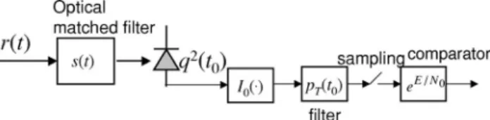
the schematic block diagram of Fig. 1. The received signal first passes through an optical matched filter having an impulse response equal to the soliton pulse of s共t兲 [or s共 −t兲 for an asymmetric pulse]. The output of the optical matched filter is q共t0兲exp共j兲. The output of the optical
matched filter converts into an electrical signal with a photodetector. The photodetector gives an output propor-tional to the square of q共t0兲2. The implementation of the
correlation of Eq. (4) by using a matched filter can be found, for example, in Ref. 9, Chap. 6. Notice that q共t0兲2
can give q共t0兲 without loss of any information. With the
output of q共t0兲2 from the photodetector, the value of
I0关2
冑
Eq共t0兲/N0兴 in expression (8) can be found. Theinte-gration in expression (8) with respect to t0is again
imple-mented using an electrical filter with an impulse response of pT共t0兲, whose output is sampled at the right time. In
Fig. 1, the probability density of pT共t0兲 does not need to be
Gaussian distributed,18,20 but it must be symmetrical with respect to zero. After the sampler, the presence or absence of the soliton is decided when compared with the scalar value of exp共E/N0兲. The filter with impulse
re-sponse of pT共t0兲 may be called an electrical matched filter
with an impulse response matched to the probability den-sity of the timing jitter. The nonlinear operation of the MLD includes the square operation of the photodetector with respect to the electric field and the calculation of
I0关2
冑
Eq共t0兲/N0兴.The block diagram of Fig. 1 is an implementation of the optimal decision rule of expression (8). The decision rule of expression (8) indicates that an optical matched filter should be used together with the processing shown in Fig. 1. In practice, an optical matched filter was used for opti-mal performance in Refs. 10,11 for the detection of a sig-nal without timing jitter. The sigsig-nal processing after the photodetector can be implemented, for example, by digital signal processing.
Practical optical and electrical components of Fig. 1 may have small differences with the decision rule of ex-pression (8) owing to implementation errors. Although we cannot list and analyze all those differences in this paper, the optimal decision rule of expression (8) is compared with the conventional implementation of the widening of the decision window.
3. PERFORMANCE EVALUATION
Without timing jitter or pT共t0兲=␦共t0兲, the right-hand side
of expression (8) becomes I0共2
冑
Eq / N0兲兩t0=0, and thedeci-sion rule of expresdeci-sion (8) can be simplified to a quadratic detector (Ref. 9, Section 8.3). The quadratic detector is
q2
0 1
qth2, 共9兲
with qth as the optimal threshold without timing jitter.
With a performance the same as that for noncoherent de-tection of an amplitude-shift keying signal, the error probability can be calculated using the well-known Mar-cum Q function.21,22 The error probability for the case without timing jitter is shown in Fig. 2 as a dashed line. The error probability of Fig. 2 is shown as a function of the SNR, given by the ratio of E / N0. The threshold of
de-tection is calculated using expression (8) with pT共t0兲
=␦共t0兲. An error probability of 10−9 requires an SNR of
about 18.9 dB for a soliton signal.
The performance of the MLD of expression (8) does not lead to a simple analytical error probability for a soliton with timing jitter. Numerical simulation is conducted when the timing jitter is zero-mean Gaussian distributed with variance oft2. The performance of the system is
de-termined by the variance of t2 and the SNR, maybe to-gether with some parameters of the signal. Both the SNR of E / N0 and the variance of the timing jitter of t
2 are
functions of the fiber link configuration. Although the cal-culation of the SNR is a standard procedure for system design, the variance oft2further depends on the method
of timing-jitter control.
The simulated error probabilities are shown in Fig. 2 withtnormalized to the FWHM of the soliton. Figure 2
shows that the MLD for a soliton with timing jitter has a small SNR penalty fortcomparable with the FWHM of
the soliton.
Fig. 1. Schematic of the MLD of the presence or absence of a soliton with timing jitter. This schematic diagram shows the implementation of the decision rule of expression (8). Comp, xxx.
Fig. 2. Simulated error probability of the MLD for a soliton with timing jitter. Various markers (except the two five-point stars) are the error probability from an importance sampling simula-tion. The two five-point stars are from a Monte Carlo error count for t= 1. The dashed line is the theoretical error probability without timing jitter. Solid curves include the walk-out probabil-ity that the timing jitter is outside the bit interval.
To investigate those cases with small error probabili-ties around 10−9, a numerical simulation cannot be
con-ducted directly using the method of Monte Carlo error count. The simulation of Fig. 2 uses importance sampling, similar to the methods of Refs. 19, 23, and 24. The re-ceived signal is a soliton with different timing jitter ac-cording to the Gaussian distribution with variance oft2. The noise sample after the optical matched filter of Fig. 1 with a time corresponding to the peak optical intensity is generated on the basis of uniform distribution. Other noise samples are generated by Gaussian distribution with a correlation depending on the optical matched filter. Each error count is weighted according to the probability difference between the actual Gaussian noise samples and the generated noise samples.19,23Other than adding a biased noise sample after the optical matched filter of Fig. 1 instead of the actual signal with amplifier noises before the filter, the numerical simulation followed closely the decision rule of expression (8). The sampling time be-fore the comparator is chosen by the optimal time to maximize the signal power for the case without both noise and timing jitter.
The error probability calculated from the simulation is shown in Fig. 2 using different markers for a timing-jitter standard deviation oft from 0.1 to 1.0 of the FWHM of
the soliton. Even with a soliton having a large timing jit-ter oft= 1.0, the SNR penalty is just about 0.2 dB
com-pared with the case without timing jitter (dashed line). Figure 2 also shows the error probability, taking into account the probability that the soliton may have a tim-ing jitter outside the bit interval whent= 0.8, 1.0 and the
bit interval is ten times the FWHM of the soliton. The bit interval of T = 10 is chosen for convenience.1Fort⬍0.8,
the walk-out probability does not affect the overall error probability and is not shown in Fig. 2. From Fig. 2, a soli-ton with a large timing jitter is mainly affected by the walk-out probability, especially for a system with a bit in-terval just four to six times the FWHM of the soliton. Un-like the receiver with widening decision window, the simulation results of Fig. 2 show that the receiver sche-matic of Fig. 1 does not give a large SNR penalty.
The importance sampling method biases the noise sam-pling after the optical matched filter to speed up the simulation. With noise samples independent of one an-other, the biasing of only one noise sample before the op-tical matched filter does not speed up the simulation. The biasing of all noise samples before the optical filter speeds up the simulation, but the evaluation of weighting is not as simple as the biasing of only one noise sample. In ad-dition to importance sampling, simulation is also con-ducted the raw method of Monte Carlo error count. The Monte Carlo error count and importance sampling match each other until the error probability of about 2⫻10−5,
mostly limited by computation resources. Figure 2 shows two simulated points for the case of t= 1 using raw
Monte Carlo count. Each Monte Carlo simulation counts at least 40 errors to ensure a narrow confident interval.24 Figure 2 shows that the method of importance sampling is accurate, at least up to the limitation of the raw Monte Carlo count.
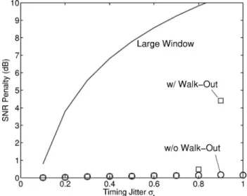
Figure 3 shows the SNR penalty as a function of a nor-malized timing jitter of t. For lengthening the decision
window, the window width must be about 12tto ensure
that the probability of the soliton’s walking-out of the de-cision window is less than erfc关w/共2t
冑
2兲兴=2⫻10−9.1Thedecision window of 12tgives 10⫻log10共12t兲 of SNR
pen-alty whent⬎0.1. For example, t= 0.5 requires a
deci-sion window width of w⬇6, corresponding to
approxi-mately 7 dB of SNR penalty. Figure 3 shows that the optimal detector is able to greatly reduce the SNR pen-alty. For the standard deviation of t⬎1, the system is
dominated by the walk-out probability. With the MLD, walk-out probability is important when t⬎0.8. For
lengthening the decision window, walk-out probability is significant whent⬎0.1.
The MLD of expression (8) or Fig. 1 has an electrical filter with an impulse response the same as the probabil-ity densprobabil-ity of pT共t0兲. The walk-out probability depends on
the tail of pT共t0兲, but the left-hand side of expression (8)
depends on the center part of pT共t0兲 around its mean of
t0= 0. Although the MLD of expression (8) depends weakly
on the timing-jitter variance oft2, the walk-out probabil-ity depends strongly ont2as from Fig. 2.
MLD is an operation in the receiver. Soliton timing jit-ter is not reduced by using MLD, but the error probability is reduced owing to better soliton detection. The MLD is more applicable when soliton control is used to allow long-distance transmission. Passing through more optical am-plifiers than systems without soliton control, the SNR for long-distance systems is reduced. With reduced SNR, the receiver does not allow a large SNR penalty.
4. CONCLUSION
The MLD of a soliton with timing jitter is derived, to our knowledge, for the first time. The MLD uses an optical matched filter preceding the photodetector and followed by nonlinear signal processing. The MLD is a process at the receiver that detects the presence or absence of a soli-ton to minimize the error probability.
With MLD, other than the walk-out probability that the soliton has a timing jitter outside the bit interval, a
Fig. 3. SNR penalty as a function of a normalized timing-jitter variance oft. The solid curve is using a widening decision win-dow. The square and circle markers are from simulation with and without including the walk-out probability, respectively.
soliton is not affected by timing jitter. Even with a timing-jitter standard deviation the same as the soliton FWHM, the SNR penalty is just about 0.2 dB. The MLD has a sig-nificantly smaller SNR penalty than a detector with a widening decision window.
K.-P. Ho, the corresponding author, can be reached by e-mail at kpho@cc.ee.ntu.edu.tw.
REFERENCES
1. J. P. Gordon and H. A. Haus, “Random walk of coherently amplified solitons in optical fiber transmission,” Opt. Lett.
11, 865–867 (1986).
2. A. Mecozzi, J. D. Moores, H. A. Huas, and Y. Lai, “Soliton transmission control,” Opt. Lett. 16, 1841–1843 (1991).
3. Y. Kodama and A. Hasegawa, “Generation of
asymptotically stable optical solitons and suppression of Gordon–Haus effect,” Opt. Lett. 17, 31–33 (1992).
4. M. Nakazawa, Y. Yamada, H. Kubota, and E. Suzuki, “10 Gbit/s soliton data transmission over one million of kilometers,” Electron. Lett. 27, 1270–1272 (1991). 5. E. Iannone, F. Matera, A. Mecozzi, and M. Settembre,
Nonlinear Optical Communication Networks (Wiley, 1998), chap. 5.
6. L. F. Mollenauer, E. Lichtman, M. J. Neubelt, and G. T. Harvery, “Demonstration, using sliding-frequency guiding filters, of error-free soliton transmission over more than 20 Mm at 10 Gbit/ s single channel, and over more than 13 Mm at 20 Gbit/ s in a two-channel WDM,” Electron. Lett.
29, 910–912 (1993).
7. M. Suzuki, H. Tanaka, N. Edagawa, and Y. Matsushima, “New applications of a sinusoidally driven InGaAsP electroabsorption modulator to in-line optical gates with ASE noise reduction effect,” J. Lightwave Technol. 10, 1912–1918 (1992).
8. L. F. Mollenauer, P. V. Mamyshev, and M. J. Neubelt, “Demonstration of soliton WDM transmission at 6 and 7 ⫻10 Gbit/s, error free over transoceanic distance,” Electron. Lett. 32, 471–472 (1996).
9. R. N. McDonough and A. D. Whalen, Detection of Signals in Noise, 2nd ed. (Academic, 1995).
10. W. A. Atia and R. S. Bondurant, “Demonstration of return-to-zero signaling in both OOK and DPSK formats to improve receiver sensitivity in an optically preamplifier receiver,” in Proceedings of IEEE Laser Electro-Optics Annual Meeting (LEOS) ’99 (IEEE, 1999), paper TuM3.
11. D. O. Caplan and W. A. Atia, “A quantum-limited optically-matched communication link,” in Optical Fiber Communication Conference, Vol. 56 of OSA Trends in Optics and Photonics Series (Optical Society of America, 2001), paper MM2.
12. A. Mecozzi, C. B. Clausen, and M. Shtaif, “Analysis of intrachannel nonlinear effects in highly dispersed optical pulse transmission,” IEEE Photon. Technol. Lett. 12, 292–294 (2000).
13. M. J. Ablowitz and T. Hirooka, “Intrachannel pulse interaction in dispersion-managed transmission systems: timing shifts,” Opt. Lett. 26, 1846–1848 (2001).
14. O. V. Sinkin, V. S. Grigoryan, R. Holzlohner, A. Kalra, J. Zweek, and C. R. Menyuk, “Calculation of error probability in WDM RZ systems in presence of bit-pattern-dependent nonlinearity and of noise,” in Optical Fiber Communication Conference, Vol. 95 of OSA Trends in Optics and Photonics Series (Optical Society of America, 2004), paper TuN4. 15. Y. S. Kivshar and B. A. Malomed, “Dynamics of solitons in
nearly integrable systems,” Rev. Mod. Phys. 61, 763–915 (1989).
16. D. J. Kaup, “Perturbation theory for solitons in optical fibers,” Phys. Rev. A 42, 5689–5694 (1990).
17. T. Georges, “Perturbation theory for the assessment of soliton transmission control,” Opt. Fiber Technol. 1, 97–116 (1995).
18. K.-P. Ho, “Non-Gaussian statistics of the soliton timing jitter due to amplifier noise,” Opt. Lett. 28, 2165–2167 (2003).
19. R. O. Moore, G. Biondini, and W. L. Kath, “Importance sampling for noise-induced amplitude and timing jitter in soliton transmission systems,” Opt. Lett. 28, 105–107 (2003).
20. C. R. Menyuk, “Non-Gaussian correction to the Gordon–Haus distribution resulting from soliton interactions,” Opt. Lett. 20, 285–287 (1995).
21. J. I. Marcum, “A statistical theory of target detection by pulsed radar,” IRE Trans. Inf. Theory IT-6, 56–267 (1960). 22. Y. Yamamoto, “Receiver performance evaluation of various digital optical modulation–demodulation systems in 0.5 -10m-wavelength region,” IEEE J. Quantum Electron.
QE-16, 1251–1259 (1980).
23. K. S. Shanmugan and P. Balaban, “A modified Monte Carlo simulation technique for the evaluation of error rate in digital communication systems,” IEEE Trans. Commun.
COM-28, 1916–1924 (1980).
24. M. C. Jeruchim, P. Balaban, and K. S. Shanmugan, Simulation of Communication Systems: Modeling, Methodology, and Techniques, 2nd ed. (Plenum, 2001).