雲端數據管理上空間索引之鍵制定格式

國

立

交

通

大

學

資訊科學與工程研究所

碩

士

論

文

雲 端 數 據 管 理 上 空 間 索 引 之 鍵 制 定 格 式

Key Formulation Schemes for Spatial Index in Cloud Data

Managements

研 究 生：許雅婷

雲端數據管理上空間索引之鍵制定格式

Key Formulation Schemes for Spatial Index in Cloud Data Managements

研 究 生：許雅婷 Student：Ya-Ting Hsu

指導教授：彭文志 Advisor：Wen-Chih Peng

國 立 交 通 大 學

資 訊 科 學 與 工 程 研 究 所

碩 士 論 文

A Thesis

Submitted to Institute of Computer Science and Engineering College of Computer Science

National Chiao Tung University in partial Fulfillment of the Requirements

for the Degree of Master

in

Computer Science July 2012

Hsinchu, Taiwan, Republic of China

雲端數據管理上空間索引之鍵制定格式

學生：許雅婷

指導教授：彭文志

國立交通大學資訊科學與工程研究所

摘

要

有鑑於雲端運算的靈活性與可擴展性，現在雲端運算被大量運用在處理大規

模的數據分析。在雲端運算中有一些雲端數據管理系統被開發來儲存資料（例

如：HBase 與 Cassandra）。這些雲端數據管理系統通常提供資料以鍵－值為一

對（Key-Value Pair）的儲存方式，每個鍵都可以用來存取相對應的值。HBase

與 Cassandra 均提供一些指令（例如：Get、Set 與 Scan）以提供使用者給定特定

鍵的情形下來得到相對應的值。現行的雲端數據管理系統直接繼承了雲端運算的

特性（例如：高度擴展性與可用性）。根據上述雲端運算的特性，雲端數據管理

系統被廣泛用來儲存網頁資訊（Web Data），特別是搜尋引擎的資料。然而，

隨著智慧型手機（Smart Phone）及基於位置的服務（Location-Based Services）

的位置不斷的變動，使得空間訊息數據（Spatial Information）在短時間內大量的

擴增。因此，如何制定現有的雲端數據管理的空間訊息數據的鍵值是一個挑戰的

問題。在本文中，我們提出一個在雲端數據管理上基於 R

+

-tree 的鍵制定格式（簡

稱為 KR

+

-index）。有了我們對於空間訊息數據的鍵制定格式，雲端數據管理系

統可以有效率的存取這些空間訊息數據。我們基於 KR

+

-index 提出兩個常被用到

的空間查詢（Spatial Index）演算法，範圍查詢（Range Query）及 k 個最近者查

詢（k-NN Query）。此外，我們實作提出的空間索引之鍵制定格式（KR

+

-index）

在 Cassandra 上並導入人造空間訊息數據以提供有效率空間查詢，range query 與

k-NN query。在實驗結果中顯示我們提出的 KR

+

-index 優於其他現有的空間索引

之鍵制定格式與 MD-HBase，特別是當空間訊息數據分布非常不平均的情形下，

提升的效率更是顯著。

Key Formulation Schemes for Spatial Index in Cloud Data Managements

Student：Ya-Ting Hsu

Advisors：Dr. Wen-Chih Peng

Institute of Computer Science

National Chiao Tung University

ABSTRACT

Due to the flexibility and scalability in cloud computing, cloud computing

nowadays plays an important role to handle a large-scale data analysis. For data

processing operations, several cloud data managements (CDMs), such as HBase and

Cassandra, are developed. Such CDMs usually provide key-value storages, where

each key is used to access its corresponding value. Both HBase and Cassandra provide

some basic operations (e.g., Get, Set, Scan) to retrieve the values via keys specified by

users. The exiting CDMs fully inherit the characteristics of cloud computing (i.e., high

scalability and availability). With the aforementioned characteristics of cloud

computing, CDMs are widely employed for Web data, especially for search engines.

However, with the proliferation of smart phones and location-based services, data

with spatial information, referring as spatial data, are dramatically increasing.

Consequently, how to formulate keys for spatial data in the existing CDMs is a

challenge issue. In this paper, we develop several key formulation schemes. In

particular, we propose a novel Key formulation scheme based on R

+

-tree (abbreviated

as KR

+

-index). With our design for keys of spatial data, the existing CDMs are able

to efficiently retrieve spatial data. In light of KR

+

-index, two spatial queries, k-NN

query and range query, are designed. Moreover, we implement the proposed key

formulation schemes on Cassandra, and import synthetic spatial data for spatial

queries. The experimental results demonstrate that KR

+

-index outperforms other

iii

誌

謝

在本論文完成的那一刻起，代表著研究所的生涯即將告一段落。這段求學期間最要感謝的是 我的指導教授 彭文志老師。在每次論文討論的過程中，彭老師總是能夠提供豐富的建議，激發 了學生很多研究的想法並解決很多難題。除此之外，彭老師讓我了解許多人生的大道理、待人處 事應有的應對進退，使我這兩年受益匪淺。期許自己可以記得這些寶貴的知識，來迎接將來的各 種挑戰。 交大資訊科學與工程研究所扎實的教學內容，讓學生在研究所生涯收穫頗豐，在此感謝任課 教授們在課程期間的傾囊相授。感謝 01 學姊每次不厭其煩地指出我研究上的缺失，總能在我迷 茫的時候為我解惑；並且在研究之餘能一起逛 costco、打羽球，為我紓解不少壓力。感謝 Young 學姊、Oshin 學長、Barry 學長、Dimension 學長、文元學長、Luc 學長、姿柔學姊、凱評學長及 小芊學姊提供研究上的經驗並在我研究的過程中給我支持與鼓勵。感謝拍拍同學與我互相討論、 切磋及互相督促及鼓勵，使得我可以盡快的趕上進度、完成論文。此外，感謝 Wallman、王堃瑋 及 Kerker 同學們的協助。還要感謝詠翔學弟、凡凱學弟、Tom 學弟們平時與我切磋羽球，一起 享受揮灑汗水的時光。感謝坐在我旁邊的宗豪學弟在最後半年的關懷、互相討論技術與經驗及偶 爾一起慢跑。也感謝守峻學弟、建志學弟平常的搞笑及貼心的幫忙。 還要感謝我的父母與弟弟，在求學的過程中給我的支持與鼓勵。最要感謝男朋友尚哲，謝謝 你的包容、體諒與陪伴，並且在我消沉的時候給予大量的支持。 最後，感謝關心我、幫助過我的人。僅以此小小成就與大家分享！ 許雅婷 謹誌

Contents

Chinese Abstract i Abstract ii Acknowledgements iii Contents iv List of Figures vi

List of Tables vii

1 Introduction 1

2 Background 7

2.1 Multi-attribute Access . . . 7

2.1.1 Range Query . . . 7

2.1.2 k-NN Query . . . . 8

2.2 Multi-dimensional Index Techniques . . . 8

2.2.1 Tree Structures . . . 8

2.2.2 Linearization . . . 10

3 Multi-dimensional Index Structure 12 3.1 KR+_{-index . . . . 12}

3.2 Insertion and Deletion . . . 15

3.3 Space Split . . . 15

3.5 k-NN Query . . . . 17

4 Experiment 20 4.1 Insert and Delete Throughput . . . 21

4.2 Range Query . . . 21

4.3 k-NN Query . . . . 26

5 Related Work 30 5.1 HBase and Cassandra . . . 30

5.1.1 Data Model . . . 30

5.1.2 Basis Operations . . . 32

5.2 Multi-dimensional Index . . . 33

List of Figures

1.1 A Hilbert curve on grids of map. . . 4

1.2 Quad-tree with M = 3. . . . 4

1.3 An key formulation in MD-HBase. . . 4

2.1 The examples of multi-attribute access. . . 7

2.2 The examples of R-trees and R+-trees. . . 8

3.1 The overview of KR+_{-index. . . . 13}

3.2 An example of KR+-index. . . 14

4.1 Distribution of synthetic data. . . 21

4.2 The sparse and dense regions of synthetic data. . . 21

4.3 The insert and delete throughput. . . 22

4.4 The range query performance of the Hilbert method. . . 22

4.5 The range query performance of the KR+_{-index. . . . 24}

4.6 The range query performance of the advanced KR+-index . . . 25

4.7 The range query performance of the Hilbert method. . . 26

4.8 The range query response time comparison of Hilbert, advanced KR+ and MD. 27 4.9 The k-NN query performance of the Hilbert method. . . . 28

4.10 The k-NN query performance of the advanced KR+-index . . . 28

4.11 The k-NN query performance of the Hilbert method. . . . 28 4.12 The k-NN query response time comparison of Hilbert, advanced KR+ and MD. 29

List of Tables

1.1 An example of check-in records. . . 2

1.2 Data in Cassandra. . . 3

1.3 Secondary index. . . 3

1.4 A key mapping for restaurants. . . 5

3.1 The relationships between the range query response time and the parameters of the KR+_{-index. . . . 14}

Chapter 1

Introduction

In recent years, mobile devices, such as smart phones and tablet computers, become pop-ular in our daily life. Simultaneously, with the increasing prevalence of Global Positioning System (GPS), a large number of location-based applications, such as Foursquare and Flickr, have been developed. People are able to share their real-time events with friends anytime and anywhere if the Internet is available. For example, people can check in to a specific location and can note their activities, and they can see their friends’ shared real-time information by the Foursquare application. Those location-based applications induce that a huge amount of multi-attribute data, which at least consist of locations and time-stamps, are dramatically increasing. In order to retrieve and manage the huge amount of multi-attribute data well, different database management systems (DBMSs) have been developed. For traditional rela-tional database management systems (RDBMSs), there are several index structures, such as k-dimensional (k-d) trees [3], quad trees [7], and R-trees [9]. However, RDBMSs is unable to deal with thousands of millions of queries efficiently. On the other hand, distributed relational database management systems (DRDBMSs) are developed and are able to deal with multi-attribute accesses. However, DRDBMSs are unable to maintain and retrieve data among servers efficiently, because DRDBMSs take much time to make data should be consistent by appropriately locking and updating data.

To deal with a huge amount of data efficiently and flexibly, cloud computing nowadays plays an important role and new cloud data managements (CDMs), which are NoSQL databases [19], have been developed. The most prevalent NoSQL CDMs, such as HBase [11], Cassandra [12] and Amazon Simple Storage [20], are developed based on a BigTable [6] management

system. Compared with DRDBMSs, these management systems have the characteristics of high scalability, high availability and fault-tolerance because they can effectively and effi-ciently handle a large number of data updates even if failure events occur. In addition, a BigTable management system stores data as ⟨key, value⟩ pairs, and thus these BigTable-like management systems can retrieve data efficiently by the following characteristics: 1) each

⟨key, value⟩ pair is stored on multiple servers; 2) each key owns multiple versions of a value.

In other words, the first characteristic benefits the efficiency of retrieving data, and the second characteristic eliminates the waiting time of making data be consistent. Due to the inherent restriction of a BigTable data structure, these management systems only support some basic operations, such as Get, Set and Scan. A Get operation retrieves values mapped by a key; a Set operation inserts/modifies values according to a corresponding key; a Scan operation returns all values mapped by a range of keys. However, these basic operations do not directly support multi-attribute accesses.

Table 1.1: An example of check-in records. cid rid rest.name rest.lat rest.lng uid time

1 p1 Friday 24.805 120.995 u1 2011/05/08

2 p1 Friday 24.805 120.995 u2 2011/08/08

3 p2 McDonald’s 24.794 121.002 u2 2011/08/30

4 p2 McDonald’s 24.794 121.002 u3 2011/10/10

5 p3 KFC 24.794 121.005 u4 2011/11/07

Multi-attribute accesses are common and required for location-based services. We illustrate multi-attribute access queries using an example. To illustrate the query example of query, we use the data of check-in records in Table 1.1 and Cassandra to be a CDM. Note that, for the first check-in record in Table 1.1, a user whose ID is u1 checked in Friday at the

geographic coordinate (24.805, 120.995) on May 8th, 2011. Based on Cassandra, the data in 1.1 are then stored as two column families in Table 1.2(a) and Table 1.2(b). Given the check-in records and a range query as “searching checked-in restaurants whose longitudes are

within [120.990, 121.004] and whose latitudes are within [23.769, 24.800] ”, a simple method

of fetching multi-dimensional data from CDMs is scanning the whole data in database and then pruning unqualified data, but this method is time-consuming and resource-intensive. To improve the efficiency of multi-attribute accesses is to pre-establish a secondary indexe for the attribute longitude and the attribute latitude as Table 1.3(a) and Table 1.3(b), respectively.

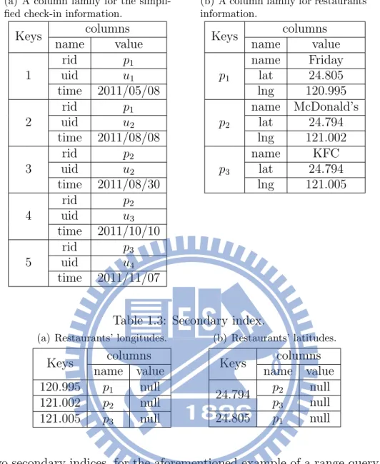
Table 1.2: Data in Cassandra.

(a) A column family for the simpli-fied check-in information.

Keys columns name value 1 rid p1 uid u1 time 2011/05/08 2 rid p1 uid u2 time 2011/08/08 3 rid p2 uid u2 time 2011/08/30 4 rid p2 uid u3 time 2011/10/10 5 rid p3 uid u4 time 2011/11/07

(b) A column family for restaurants’ information. Keys columns name value p1 name Friday lat 24.805 lng 120.995 p2 name McDonald’s lat 24.794 lng 121.002 p3 name KFC lat 24.794 lng 121.005

Table 1.3: Secondary index.

(a) Restaurants’ longitudes.

Keys columns name value 120.995 p1 null 121.002 p2 null 121.005 p3 null (b) Restaurants’ latitudes. Keys columns name value 24.794 p2 null p3 null 24.805 p1 null

With the two secondary indices, for the aforementioned example of a range query, we can get which restaurants are locate in the range. Specifically, we perform an operation of Scan on the longitudes’ secondary index to derive a set of restaurant IDs in which each corresponding restaurant’s longitude is within [120.990, 121.004] (e.g., {p1, p2}), and we similarly perform an

operation of Scan on the latitudes’ secondary index to derive a set of restaurant IDs in which each corresponding restaurant’s latitude is within [23.769, 24.800] (e.g., {p2, p3}). We then

intersect the two sets to derive a set of qualified restaurants (e.g., {p2} restaurant). However,

this index method is space-consuming for constructing a secondary index for each attribute of data, and it is time-consuming for updating secondary index structures while data were updated. To overcome the former disadvantage, a better index method is using space-filling

curves [4], such as Z-ordering [14] and Hilbert curve [5]. This kind of index methods transform multi-dimensional data into a one-dimensional space. The map was divided into 2n· 2n _grids

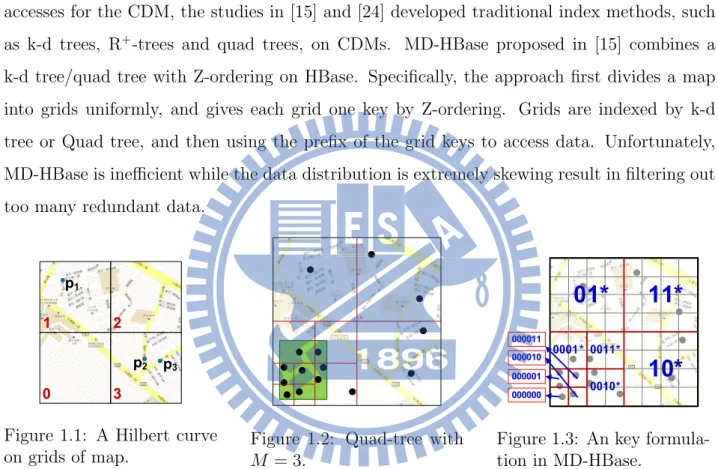
that are assigned values as keys by space-filling curves. Data in the same grid are mapped to the same key, as shown in Figure 1.1 and Table 1.4. However, the response time of a Get operation increases exponentially as the volume of data mapped by a key increases. In addition, the user-generated data usually have a skewed distribution, e.g., most people likely checked in at popular attractions. Therefore, this kind of index methods are inefficient when a distribution of data is extremely skewed. Furthermore, to support efficient multi-attributes accesses for the CDM, the studies in [15] and [24] developed traditional index methods, such as k-d trees, R+_{-trees and quad trees, on CDMs. MD-HBase proposed in [15] combines a}

k-d tree/quad tree with Z-ordering on HBase. Specifically, the approach first divides a map into grids uniformly, and gives each grid one key by Z-ordering. Grids are indexed by k-d tree or Quad tree, and then using the prefix of the grid keys to access data. Unfortunately, MD-HBase is inefficient while the data distribution is extremely skewing result in filtering out too many redundant data.

Figure 1.1: A Hilbert curve on grids of map.

Figure 1.2: Quad-tree with

M = 3.

Figure 1.3: An key formula-tion in MD-HBase.

In this paper, to support efficient multi-attribute accesses of skewed data on CDMs, we proposed a novel multi-dimensional index, called KR+_{-index, on CDMs by designing Key}

names for leaves of R+_{-tree. A challenge issue is to filter out data after querying result from}

large difference of volume of data between grids. In order to describe conveniently, we called the size of a gird as the volume of data in the grid. However, dividing a map more meticulously could reduce the differences of the grid sizes but it also reduces the efficiency of accessing data. For example, for a range query, we need to retrieve more grids for the same spatial range. According to the aforementioned observations, we expect the differences of the grid sizes could

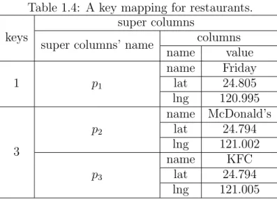
Table 1.4: A key mapping for restaurants. keys

super columns

super columns’ name columns

name value 1 p1 name Friday lat 24.805 lng 120.995 3 p2 name McDonald’s lat 24.794 lng 121.002 p3 name KFC lat 24.794 lng 121.005

be smaller and the time of grid accesses could be less at the same time. Consequently, how to divide a map into grids to reach a balance between the two points plays an important role for CDMs. In this paper, we first use R+_{-tree [18] to divide data, and the rectangles in the}

leave nodes of the tree index are treated as dynamic grids. The reasons of using R+-tree are describes as follows. First, we could get a balance between the grids sizes and the times of grid accesses by adjusting two parameters, M and m, of the R+-tree. Second, compared with other variants of the R-tree, the leaf nodes of R+_{-tree do not overlap with each other, and}

thus it is benefit for no redundant retrieving the same data from different keys and easy to define different keys for each rectangle of a leaf node. Moreover, the second challenge is how to design key names of these grids to support efficient queries on BigTable management systems. We observed the characteristics of CDMs as follows: a CDM has a fast key-value search and to Scan keys which are ordered by a dictionary order is fast. Based on these characteristics, we propose an approach to define the key name of a grid to support efficient queries. In the experiment, we implement the proposed index on two well-known CDM systems, HBase and Cassandra, and we compare the performance of the proposed index with the existing index methods. The experimental results demonstrate that our proposed index outperforms the existing index methods via skewed data.

We summarize the contributions of this paper as follows:

ˆ We propose an efficient multi-dimensional index structure, KR+_{-index, on CDMs to}

ˆ Based on KR+_{-index, we define new efficient spatial query algorithms, range query and}

k-NN query.

ˆ The KR+_{-index uses the characteristics of CDMs effectively.}

ˆ The experimental results show that the proposed KR+_{-index outperforms than other}

competitors.

The remainder of the paper is organized as follows. First, we illustrate the background of multi-attribute access, multi-dimensional index and Hilbert curve Section 2. We next propose the KR+_{-index in Section 3. In Section 4, we evaluate the performance of the proposed}

KR+_{-index for multi-attribute accesses on CDMs. Finally, we conclude the paper and give a}

Chapter 2

Background

2.1

Multi-attribute Access

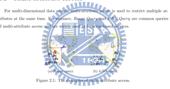
For multi-dimensional data search, multi-attribute access is used to restrict multiple at-tributes at the same time. For instance, Range Query and k-NN Query are common queries of multi-attribute access and are widely used in location-based services.

(a) Range query. (b) k-NN query.

Figure 2.1: The examples of multi-attribute access.

2.1.1

Range Query

Given a set of data points P and a spatial range R, a range query can be formulated as “searching the data points in P that locate in the spatial range R”. Note that, in this paper, each data point has location information, e.g., a longitude and a latitude. Without loss of generality, in this paper, a spatial range is represented by a rectangular range.

For instance, in Figure 2.1(a), given 15 restaurants, marked by gray points, and a red query range R, the range query is to search which restaurants locate in the range R. As shown in

Figure 2.1(a), the result of the range query is {p1, p2, p3, p4, p5}.

2.1.2

k-NN Query

Given a set of data points P , a query location p = (px, py) and a constant k, a k-NN query

can be formulated as “searching the data points in P that are the k nearest data points of p”. For example, in Figure 2.1(b), given 15 restaurants, a user-specified location p marked by the red color and k = 5, a 5-NN query here is to search five nearest restaurants of p. Thus, the search result of this query is {p4, p5, p6, p7, p8} shown in Figure 2.1(b).

2.2

Multi-dimensional Index Techniques

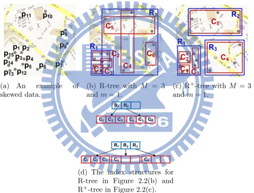
(a) An example of skewed data. (b) R-tree with M = 3 and m = 1. (c) R+_{-tree with M = 3} and m = 1.

(d) The index structures for R-tree in Figure 2.2(b) and R+_{-tree in Figure 2.2(c).}

Figure 2.2: The examples of R-trees and R+-trees.

2.2.1

Tree Structures

R-tree, developed for indexing multi-dimensional data, are widely used in multi-attribute accesses. For instance, given fifteen checked-in restaurants in Figure 2.2(a), a R-tree index structure with two parameters M = 3 and m = 1 can be stored as shown in Figure 2.2(b) and

the top figure in Figure 2.2(d). Note that M and m are used to restrict that the number of elements of a node in a tree is in [m, M ]. Because R-tree is a balance search tree by dynamically splitting and merging nodes and R-tree can restrict the number of elements in each node by controlling the M and m, R-tree benefits for searching skewed data. Moreover, to efficiently index different multi-dimensional data, different variations of R-trees have been developed, such as R+_{-tree [18], R}∗_{-tree [2] and the Hilbert R-tree [10]. The R}+_{-tree developed a new}

rule of splitting and merging nodes to speed up the multi-attribute accesses. For instance, given a set of data points in Figure 2.2(a), Figure 2.2(c) shows an example of R+_{-tree with}

M = 3 and m = 1, and the corresponding index structure is illustrated in the bottom figure

in Figure2.2(d). As shown in Figure 2.2(c), the rectangles do not overlap with each other, and it benefits to reduce searching time. The reason is that, compared with R-trees, we do not search duplicated results using R+_-trees.

R-tree, developed for indexing multi-dimensional data, are widely used in multi-attribute accesses. For instance, given fifteen checked-in restaurants in Figure 2.2(a), a R-tree index structure with two parameters M = 3 and m = 1 can be stored as shown in Figure 2.2(b) and the top figure in Figure 2.2(d). Note that M and m are used to restrict that the number of elements of a node in a tree is in [m, M ]. Because R-tree is a balance search tree by dynamically splitting and merging nodes and R-tree can restrict the number of elements in each node by controlling the M and m, R-tree benefits for searching skewed data. Moreover, to efficiently index different multi-dimensional data, different variations of R-trees have been developed, such as R+-tree [18], R∗-tree [2] and the Hilbert R-tree [10]. The R+-tree developed a new rule of splitting and merging nodes to speed up the multi-attribute accesses. For instance, given a set of data points in Figure 2.2(a), Figure 2.2(c) shows an example of R+-tree with

M = 3 and m = 1, and the corresponding index structure is illustrated in the bottom figure

in Figure2.2(d). As shown in Figure 2.2(c), the rectangles do not overlap with each other, and it benefits to reduce searching time. The reason is that, compared with R-trees, we do not search duplicated results using R+-trees.

Quad-trees [7] are another common tree structures for indexing multi-dimensional data. In quad-trees, each internal node has exactly four children. However, quad-trees are not balance trees because a region is split into four sub-regions until the number of data points in the region is less than or equal to a given parameter M . For instance, given the data in Figure

2.2(a), Figure 1.2 shows an quad-tree with M = 3. However, quad-trees do not benefit for skewed data. For example, given a query range marked by the green color in Figure 1.2, for the range query, the searching time of using quad-trees is greater than the searching time of using R+_{-tree, because the depth of the quad-tree structure is higher than the depth of the}

R+-tree structure.

Quad-trees [7] are another common tree structures for indexing multi-dimensional data. In quad-trees, each internal node has exactly four children. However, quad-trees are not balance trees because a region is split into four sub-regions until the number of data points in the region is less than or equal to a given parameter M . For instance, given the data in Figure 2.2(a), Figure 1.2 shows an quad-tree with M = 3. However, quad-trees do not benefit for skewed data. For example, given a query range marked by the green color in Figure 1.2, for the range query, the searching time of using quad-trees is greater than the searching time of using R+-tree, because the depth of the quad-tree structure is higher than the depth of the R+_{-tree structure.}

2.2.2

Linearization

Linearization is a well-known technique for indexing multi-dimensional data by transform-ing multi-dimensional data into one-dimensional data. One of the most popular method of linearization is using space-filling curves, such as Hilbert curve and Z-ordering. Given a two-dimensional data, this method first divides the map into 2n_·2n_{non-overlapping grids, where n}

is a parameter, and assign a number for each grid according to the order of traversing all grids. Note that the number of each grid is regarded as a key. Figure 1.1 illustrates an example of linearization using Hilbert curve with 21 · 21 _{grids. In Figure 1.1, the map is divided into}

four grids, and the keys of these grids are represented by 0, 1, 2 and 3 according to Hilbert curve. However, using space-filling curves to index data may be not efficient. Take check-in records indexing for an example. If a value of n is set to be lower, it induces a larger size of a grid, and a grid would possibly cover more check-in records distributed in the area of the grid. Given a range query, all check-in records locating in the grids overlapping the range would be retrieved, and then these records are further verified whether they are indeed in the query range. Therefore, it would result in that more unqualified check-in records, said false-positive, should be pruned, and it takes more time to derive the query result. On the other hand, if n

is set to be larger, it would increase the times to retrieve more grids. Thus, for this indexing technique, it is a trade-off to set a proper value of n for efficiency.

Linearization is a well-known technique for indexing multi-dimensional data by transform-ing multi-dimensional data into one-dimensional data. One of the most popular method of linearization is using space-filling curves, such as Hilbert curve and Z-ordering. Given a two-dimensional data, this method first divides the map into 2n·2n_{non-overlapping grids, where n}

is a parameter, and assign a number for each grid according to the order of traversing all grids. Note that the number of each grid is regarded as a key. Figure 1.1 illustrates an example of linearization using Hilbert curve with 21 · 21 grids. In Figure 1.1, the map is divided into four grids, and the keys of these grids are represented by 0, 1, 2 and 3 according to Hilbert curve. However, using space-filling curves to index data may be not efficient. Take check-in records indexing for an example. If a value of n is set to be lower, it induces a larger size of a grid, and a grid would possibly cover more check-in records distributed in the area of the grid. Given a range query, all check-in records locating in the grids overlapping the range would be retrieved, and then these records are further verified whether they are indeed in the query range. Therefore, it would result in that more unqualified check-in records, said false-positive, should be pruned, and it takes more time to derive the query result. On the other hand, if n is set to be larger, it would increase the times to retrieve more grids. Thus, for this indexing technique, it is a trade-off to set a proper value of n for efficiency.

Chapter 3

Multi-dimensional Index Structure

The CDMs provide key-value search, which retrieving a value by given a key, based on the data model of CDMs. The CDMs support basic operations to access data, but these operations do not directly support multi-attribute access. To deal with the problem of multi-attribute access, we develop a multi-dimensional index structure for CDMs. Furthermore, in this paper, we apply our developed index structure for range query and k-NN query on CDMs.

3.1

KR

+

-index

Our design of multi-dimensional index is based on the observation of CDMs. We observe three characteristics of CDMs: 1) the time of retrieving a key that has n data is far less than the time of retrieving n keys that each has one data; 2) the time of retrieving a key has n data increases more than twice as n is large. 3) the operation Scan is more efficient than multiple Get that both retrieving the same keys. Considering the aforementioned characteristics, for a query should make the number of false-positive to be smaller from the characteristic 2 and let the number of sub-queries to be smaller from the characteristic 1. R+-tree is balance tree that has M and m to control the size of each dynamic rectangle, we could use the M and m to meet the trade-off between false-positive and sub-queries. Considering the characteristic 3, we use the Hilbert curve to let the queried key to be as continuous as possible and then the rate of Scan is increased.

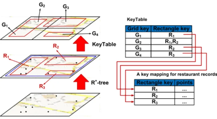
Figure 3.1 is the framework of KR+_{-index. First, the data is constructed by the R}+_-tree

Figure 3.1: The overview of KR+_-index.

In order to retrieve the restaurant records efficiently, we proposed a mapping method for retrieving the queried rectangle keys. Second, the map is divided into 2n _{× 2}n _non-overlap

grids, {G1, G2, G3, G4}, uniformly. Then, for each grid maintains a list of rectangles that

overlap with this grid. For instance, the grid G2 overlaps with rectangles {R1, R2} that

the KeyTable store a record ⟨G2, {R1, R2}⟩. Thus, a query could convenient transform into

which grids need to be queried and then through the KeyTable could easily get the required rectangles.

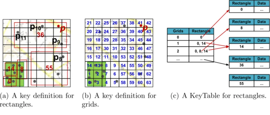
For these key-value storages, it is crucial to define the key, because we use the key to access corresponding data. We construct R+-tree to discover non-overlap minimum bound-ing rectangles. Considerbound-ing the characteristic 3, we use Hilbert-curve to define the keys, since Hilbert-curve manifests superior data clustering compared with other multi-dimensional linearization technique. For each leaf rectangle, we use the Hilbert-value of the geographic coordinate of the centroid of rectangle be the key. Then, we split the space to non-overlap 2n_{× 2}n _{grids uniformly and each grid has a value which is transformed by}

Hilbert-curve. Take the Figure 3.2(a), for example, each rectangle is given a Hilbert value. Each grid also given a Hilbert value, the grid 1 in Figure 3.2(b) overlaps with the rectangles {0,

14} that ⟨1, {0, 14}⟩ is stored in KeyTable as showed in Figure 3.2(c). We could get the

rectangle information though the KeyTable and the multi-attribute access can retrieve the data efficiently.

The decision of (M, m) and order will affect the efficiency of range query. Thus, we decided to dynamically generate the values of (M, m) and order. We knew that (M, m) influence the size of rectangles and the order decided the grid size. We observed the relationship between the response times and the parameters, (M, m) and o. As showed in Table 3.1, this

(a) A key definition for rectangles.

(b) A key definition for grids.

(c) A KeyTable for rectangles.

Figure 3.2: An example of KR+_-index.

is the average length and width of rectangles of ten million data size and the length of grids with different order; the average length and width of (M, m) = (250, 125) is closed to the grid length of order 7, and the range query response times of KR+-index, showed in Figure 4.5(b), expressed the range query with fixed (M, m) = (250, 125) had better response time as order o = 7. We found that the closer the rectangle size and the grid size, the better the response time of range query. Thus we proposed a new method, called advanced KR+

-index, a KR+-index of automatically determines the size of the parameters. It first decides a small value of (M, m), and evaluates the average size of the size of rectangles, then calculates the closest grid size generated by order. The objective function of o can be expressed as

o = mino(|len(o) − avgLen(M)| + |len(o) − avgW id(M)|) Thus, it determines the (M, m) and

order automatically.

Table 3.1: The relationships between the range query response time and the parameters of the KR+_-index.

(a) Average length and width of rectangles of KR+_-index.

M m avg. len. avg. wid.

50 25 1128.4283 2656.2368 100 50 4928.2417 4671.1948 250 125 6941.6216 6280.1025

(b) The length and width of grids with dif-ferent order.

order len.

6 15625

7 7812.5

3.2

Insertion and Deletion

The algorithm to insert a new data point as showed in Algorithm 2. It first loops up, using Algorithm 1, the key of node corresponding to the node to which the point belongs, and then inserts the data point into node. Since there is a upper bound to the number of points in the node, the insertion algorithm checks the current size of node to determine if a split is needed. The deletion algorithm showed in Algorithm 3 is similar to the insertion. It first loops up the key of node corresponding to the node to which the point belongs, and then deletes the data point from node.

Algorithm 1 Subspace Lookup

1: /* p = (x, y) is a data point. */;

2: /* o is the Hilbert order. */;

3: i←x mod o;

4: j←y mod o;

5: return Hilbert(i,j);

Algorithm 2 Insert a new data point

1: /* p is a new data point. */;

2: key← SubspaceLookup(p);

3: InsertToKRPlust(key,p);

4: if Size(key)>MaxNodeSize then

5: SplitSpace(key);

6: end if

Algorithm 3 Delete a data point

1: /* p is a new data point. */;

2: key← SubspaceLookup(p);

3: DeleteFromKRPlust(key,p);

3.3

Space Split

R+_{-tree limits the number of points contained in each node; a node is split when the}

number of points in a node exceeds this limit. We set the maximum number of points in a node with 50, 100 and 250, and the maximum number of points of insertion performance is set by 50 in the experiments. A split in the R+_{-tree relies on the key definition of each node,}

the old node that the points in the old node will be allocated into one of the new sub-node. The number of new nodes created depends on the index structure used: a R+_{-tree split a node}

in one dimension, the opposite is to let the data points determine of the hyperplane, as the k-d trees [3] or k-d-b trees [17] do. For every dimension split, the name of the new sub-node is created by the Hilbert code of the center points of the new sub-node. Algorithm 4 shows the pseudocode for sub-node name generation following a split.

Algorithm 4 Split node

1: /* ns is a node of R+_{-tree */;}

2: /* na, nb are two new node split from node ns by R+-tree */;

3: keyOfNa←Hilbert(center points of na);

4: keyOfNb←Hilbert(center points of nb);

5: for each point p in ns do

6: if p in na then 7: pointsOfNa.add(p); 8: else 9: pointsOfNb.add(p); 10: end if 11: end for 12: Insert(keyOfNa, pointsOfNa); 13: Insert(keyOfNb, pointsOfNb); 14: Delete(keyOfNs);

3.4

Range Query

The multi-dimensional range query is commonly used in location based applications. Al-gorithm 5 is the pseudo code for range query in HBase and Cassandra. (pl, ph) is the range

for the query, pl is the lower bound and ph is the upper bound. Hilbert curve splits the space

into grids, and each grid has one grid key. The algorithm first compute the coordinate of grids overlap with the range query. The GridKeys is the set of grid keys contained in the query range. For each coordinate of grid c, the function ComputeContainGridKeys() computes the corresponding grid keys via Hilbert curve and add to the list, GridKeys. Then, according to the key table we could find the rectangle keys in the query range. Line 5-8 find the queried key and line 9-10 fetch the points in the corresponding key. The function GetContainPoint() returns the queried data by first retrieving points from Cassandra and HBase with key k and then filtering out some points that is not in the query range.

Algorithm 5 Range Query

Input: pl, ph: the range for the query;

Output: points contained in the range;

1: Coordinate← ComputeCoordinateOfGrid(pl, ph);

2: Keys ← ϕ;

3: RectKeys ← ϕ;

4: Result← ϕ;

5: for each Coordinate c∈Coordinate do

6: GridKeys← GridKeys ∪ComputeContainGridKeys(c));

7: end for

8: RectKeys← GetRectKeys(GridKeys);

9: for each Key k∈RectKeys do

10: Result← Result ∪GetContainP oints(k));

11: end for

12: return Result;

Algorithm 6 GetRectKeys(GridKeys)

Input: GridKeys: the grid keys overlap with query range;

Output: the rectangle keys overlap with query range;

1: RectKeys ← ϕ;

2: for each grid key gk ∈GridKeys do

3: RectKeys← RectKeys ∪ KeyTable(gk));

4: end for

5: return RectKeys;

As shown in Figure 3.2, take the green block as range query that we will show an example how range query works. Using the query range to get the geographic coordinates of the overlapped grids, {(0, 0), (0, 1), (0, 2), (1, 0), (1, 1), (1, 2), (2, 0), (2, 1), (2, 2)}, then get the Hilbert values of each geographic coordinate, {0, 3, 4, 1, 2, 7, 14, 13, 8}. Second, getting keys of rectangles through the KeyTable that grid 0 maps to rectangle {0}, grid 1 maps to rectangles {0, 14}, grid 1 maps to rectangles {0, 8, 14}, etc. Thus, we can get the queried rectangle keys,{0, 8, 14}, by union the rectangle sets got from the former steps. Finally, using the rectangle keys to retrieve data in the CDMs and then pruning the unqualified data to get the query result.

3.5

k-NN Query

The k-NN query is also commonly used in location based applications. Algorithm 7 shows the k-NN query algorithm in HBase and Cassnadra, K stores the result k nearest neighbors,

QueryRect stores the rectangles could be scanned, dist is the range for rectangle search, Rectscanned stores the rectangles had been scanned, and the data structure of QueryRect is

a queue. The k-NN query has two mainly parts: 1) set a range dist to search for rectangles overlap with a square range with centroid p and edge length 2·dist; 2) pick the nearest rectangle of p that is not scanned and add the nearest points in this rectangle into K. The algorithm keep repeat step 1, 2 until the distance of k-th nearest point and p is less than or equal to dist. The part 1) in Algorithm 7 is in line 6-11, where RectInRegion() is used to find the rectangles in square range and line 9 push the rectangles have not be scanned into QueryRect; 2) is in line 12-18, where line 12 pop the nearest rectangle, line 14 will add the points of R into K. The function RectInRegion(c, dist) in Algorithm 8 finds the rectangles overlap with the input square. It is designed by our methods for defining key in rectangles. Line 6-8 find the grids keys which overlap with the square and line 10 returns the rectangles overlap with grids through checking the KeyTable.

Algorithm 7 k-NN Query

Input: k: k nearest neighbors; p = (x, y): query point;

Output: k nearest neighbors of (x, y);

1: K← ϕ; 2: QueryRect ← ϕ; 3: dist ← 0; 4: Rectscanned ← ϕ; 5: loop 6: if QueryRect== ϕ then

7: Rectnext←RectInRegion(p,dist)−Rectscanned;

8: for each Rectangle R∈Rectnext do

9: Push(R, MinDist(p, R), QueryRect);

10: end for

11: end if

12: R←Pop(QueryRect);

13: for each Point t∈R do

14: K← K ∪ ¡t, Dist(p, t)¿ and sort K by dist;

15: end for

16: if dist(k-th point in K, p)≤ dist then

17: break;

18: end if

19: Rectscanned←Rectscanned

∪ R;

20: dist←Max(dist, MaxDist(p, R));

21: end loop

22: return K;

Algorithm 8 RectInRegion(p,dist)

Input: p = (x, y): query point; dist: means a square with edge length 2·dist and with p as its

centroid o = order: the order of Hilbert;

Output: the keys of rectangles overlap with the input rectangle

1: RectKeys ← ϕ; 2: xl ←(x-dist) mod o; 3: xh←(x+dist) mod o; 4: yl ←(y-dist) mod o; 5: yh←(y+dist) mod o; 6: for i=xl→ xh do 7: for j=yl→ yh do

8: GridKeys ← GridKeys ∪ Hilbert(i, j);

9: end for

10: end for

11: return RectKeys←KeyTable(GridKeys);

First, we will get a rectangle 36 through KeyTable with a square range of length 2·dist and then insert the location points {p9, p10, p11} of rectangle 36 into K, in that location points

are ordered by the distance from p. Second, resizing the dist to the minimum distance of k-th/—K—-th location points in K from p, the dist=dist(3-th location point in K, p) in this example. The algorithm continues the first and second steps, it will add the rectangle 55 into Rectnext and add the location points in rectangle 55 into K. The algorithm is stoped by

dist(3-th location point in K, p) ≤ dist, and we get the fist three location points {p10, p9, p8}

Chapter 4

Experiment

In this section, we will show the experiments about the time of range query and k-NN query on Cassandra with the different implementations, a base implementation using Hilbert curve for linearization(Hilbert) without any specialized index and KR+_{-index(KR) as described in}

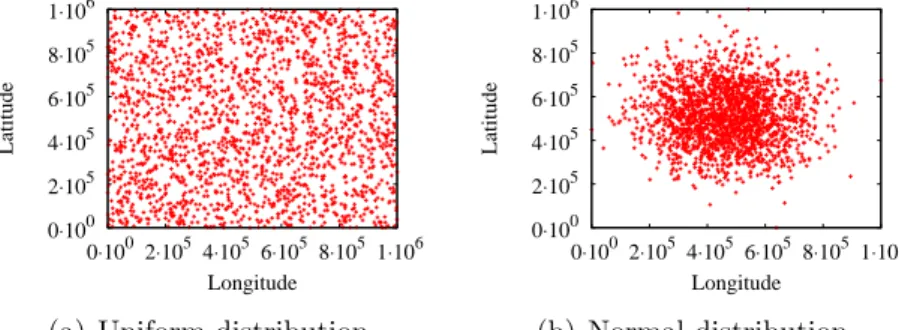
Section 3, and compare our methods with MD-HBase(MD). Our experiments were performed on a ring of Cassandra with version 1.0.10 of ten nodes that each of the two nodes on a physical machine. Each physical machine consists of two virtual machines, 2GB memory and 500GB HDD and 64bit Ubuntu 8.04.4. Our evaluation uses synthetically generated data sets primar-ily due to the need for huge data sets(gigabytes) and the need to control different aspects, such as skew and distribution, to better understand the behavior of the system. Evaluation using real data is left for future work. The synthetic data generator proposed by Yaling and Osmar[16] has two kinds of distribution, normal and uniform. The multivariate uniform dis-tribution data is simply generated with each one-dimensional uniform disdis-tribution separately, since the joint distribution of two or more independent one-dimensional uniform distributions is also uniform. The multivariate normal distribution data is generated by first producing two-dimensional uniform distribution then using the Box-Muller transformation[22][1] to transform the two-dimensional uniform distribution to a two-dimensional bivariate normal distribution with mean µ = 0 and variance σ2 _{= 1. We generated synthetic data of uniform and}

nor-mal distribution of one cluster with data size equals to two hundred thousand, five hundred thousand and one million on a square map of one million units of length, as showed in Figure 4.1(a) 4.1(b).

0⋅100 2⋅105 4⋅105 6⋅105 8⋅105 1⋅106 0⋅100 2⋅105 4⋅105 6⋅105 8⋅105 1⋅106 Latitude Longitude

(a) Uniform distribution.

0⋅100 2⋅105 4⋅105 6⋅105 8⋅105 1⋅106 0⋅100 2⋅105 4⋅105 6⋅105 8⋅105 1⋅106 Latitude Longitude (b) Normal distribution.

Figure 4.1: Distribution of synthetic data. Figure 4.2: The sparse and dense regions of synthetic data.

4.1

Insert and Delete Throughput

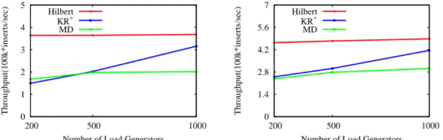
Supporting high insert throughput of data updates is critical to sustain the large numbers of location based services. We evaluated the insert performance on a Cassandra cluster with ten commodity nodes. Figure 4.3(a) plots the insert throughput as a function of the load on the system. We varied the number of load generators with 200, 500 and 1000; each generator created a load of 1000 inserts per second. We use the synthetic data using a Normal distribution with mean µ = 0 and variance σ2 = 1. Using synthetic data allow as to control the skew of large data sets. All of the methods showed good scalability; the throughput is at least 150k location data points per second. The lower throughput of KR+ and MD is the cost of associated with the splitting nodes on R+_{-tree and quad tree. On the other hand,}

the Hilbert does not need splitting nodes. On the average, the KR+ needs about 25 seconds to split a node and the MD needs about 40 seconds. The dataset and the number of load generators used in deletion is the same as insertion. The delete throughput, as showed in Figure 3 is higher than insert throughput, but the performance comparison seems similar between Hilbert, KR+ and MD. The KR+ and MD have lower throughput since more cost of merging nodes on R+_{-tree and quad tree.}

4.2

Range Query

We now evaluate range query performance using the different implementations of the in-dex structures, a base implementation using Hilbert curve for linearization(Hilbert) without

0 1 2 3 4 5 200 500 1000 Throughput(100k*inserts/sec)

Number of Load Generators Hilbert

KR+ MD

(a) The insert throughput as a function of the load on the system.

0 1.4 2.8 4.2 5.6 7 200 500 1000 Throughput(100k*inserts/sec)

Number of Load Generators Hilbert

KR+ MD

(b) The delete throughput as a function of the load on the system.

Figure 4.3: The insert and delete throughput.

any specialized index and KR+_{-index(KR) as described in Section 3, and compare our}

meth-ods with MD-HBase(MD). We generated six datasets using model of normal and uniform distribution that for each distribution generate sizes of two hundred thousand, five hundred thousand and one million points. We executed the range queries on a ten-node Cassandra cluster in five machines. The response time of each range query with same set of parameter values were performed one hundred times random queries on normal distribution of dense region(Normal-dense), normal distribution of sparse region(Normal-sparse) and uniform distribution(Uniform). The dense region is located in the map center with ten hundred thou-sand unit of length and the sparse region is others, as showed in Figure 4. We evaluate the range query with a square size equals to ten thousand units of length, five thousand units of length and one million units of length.

0 2 4 6 8 10 10000 50000 100000 Time(s)

Query length(units of length) Uniform

Normal-sparse Normal-dense

(a) The range query response times for Hilbert of varying query size. 0 4 8 12 16 20 5 6 7 8 Time(s) Order Uniform Normal-sparse Normal-dense

(b) The range query response times for Hilbert of varying order.

0 2 4 6 8 10 200000 500000 1e+006 Time(s)

Data size(# of points) Uniform Normal-sparse Normal-dense

(c) The range query response times for Hilbert of varying data size.

Figure 4.4: The range query performance of the Hilbert method.

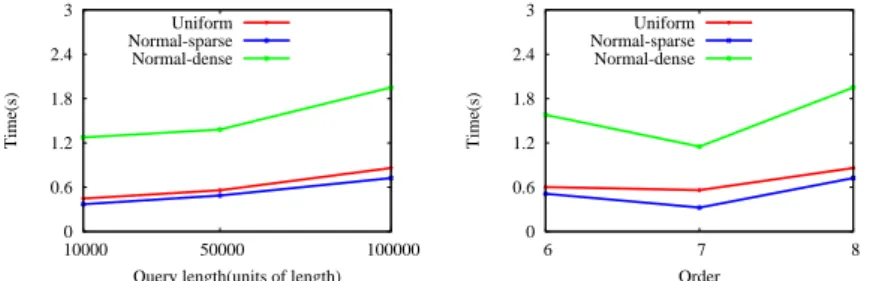
The Hilbert method has a parameter order o, which is used to decide how many grids were divided from map as mentioned in Section 2. The order we evaluated in range query of Hilbert are o = {5, 6, 7, 8}. Figure 4.7 plots the range query response times for the Hilbert

method of varying query size, order and data size respectively. Figure 4.4(a) plots the range query response times of varying query size with fixed data size ds = 1000000 and order o = 7. Figure 4.4(b) plots the range query response times of varying order with fixed query square size of length qs = 100000 and data size ds = 1000000. Figure 4.4(c) plots the range query response times of varying data size with fixed query square size of length qs = 100000 and order o = 7. The plots with other arguments, such as the response times of different arguments combination of ds = {200000, 500000} and o = {5, 6, 8} are extremely similar to Figure 4.7, so those are not displayed to save the space. As showed in Figure 4.4(a), the larger the query size, the larger the response time, since the number of fetched points increased. As is evident from Figure 4.4(b), there is a lower bound as o = 7, the response time is increased as the order increased larger than 7 and the order decreased lower than 7. This is reasoned by the trade-off between the false-positive ratio and the number of sub-queries. This means that the number of sub-queries increased as the order increased more than 7 and the false-positive ratio increased as the order decreased less than 7, thus both led to response time increased. In Figure 4.4(c), the response time increased as the data size increased. In three plots of Hilbert, the response times of normal-dense region are very poor compared with the other region and distribution.

The KR+_{-index method has three parameter, the lower bound and upper bound of}

rect-angles (M, m) and the order o. The lower bound and upper bound of rectrect-angles we evaluated in range query of the KR+_{-index are (M, m) = {(50, 25), (100, 50), (250, 125)}, and the}

or-der are o = {6, 7, 8}. Figure 4.5 plots the range query response times for the KR+-index of varying query size, order, data size and (M, m). Figure 4.5(a) plots the range query response times of varying query size with fixed data size ds = 1000000, (M, m) = (250, 125) and order

o = 8. Figure 4.5(b) plots the range query response times of varying order with fixed data

size ds = 1000000, query square size of length qs = 100000 and (M, m) = (250, 125). Figure 4.5(c) plots the range query response times of varying data size with fixed query square size of length qs = 100000, (M, m) = (250, 125) and order o = 8. Figure 4.5(d) plots the range query response times of varying (M, m) with fixed query square size of length qs = 100000, data size ds = 1000000 and order o = 8. The plots with other arguments, such as the re-sponse times of different arguments combination of ds = {200000, 500000}, o = {6, 8} and (M, m) = {(100, 50), (50, 25)} are extremely similar to Figure 4.7, so those are not displayed

0 0.6 1.2 1.8 2.4 3 10000 50000 100000 Time(s)

Query length(units of length) Uniform

Normal-sparse Normal-dense

(a) The range query response times for KR+_{-index of varying}

query size. 0 0.6 1.2 1.8 2.4 3 6 7 8 Time(s) Order Uniform Normal-sparse Normal-dense

(b) The range query response times for KR+_{-index of varying}

or-der. 0 0.6 1.2 1.8 2.4 3 200000 500000 1e+006 Time(s)

Data size(# of points) Uniform Normal-sparse Normal-dense

(c) The range query response times for KR+_{-index of varying data size.}

0 0.6 1.2 1.8 2.4 3 50 100 250 Time(s) M Uniform Normal-sparse Normal-dense

(d) The range query response times for KR+_{-index of varying}

(M, m).

Figure 4.5: The range query performance of the KR+_-index.

to save the space. In Figure 4.5(a), the larger the query size, the larger the response time, since the number of fetched points increased; the same as the range query response times of varying data size, as showed in Figure 4.5(c). As showed in Figure 4.5(b), there is a trade-off between the false-positive ratio and the number of sub-queries as varying order. The response time increased as the order larger than 7, owing to spend a lot of time in fetching sub-queries; the response time increased as the order less than 7, since spending much time in pruning points do not in query range. It is the same as the range query response time of varying (M, m).

The decision of (M, m) and order will affect the efficiency of range query. Thus, we de-cided to dynamically generate the values of (M, m) and order. We observed the relationship between the response times and the parameters, (M, m) and o. We knew that (M, m) in-fluence the size of rectangles and the order decided the grid size. We found that the closer the rectangle size and the grid size, the better the response time of range query, as men-tioned in Section 3. About the setting of (M, m), we evaluate the range query of varying (M, m) = (50, 25), (100, 50), (250, 125), (1250, 625), (2500, 1250), (2500, 5000). As the

discus-sion in Section 3, the (M, m) has a lower bound at (100, 50), the response times of range query was very worse as (M, m) = (1250, 625), (2500, 1250), (2500, 5000), but the response time has a little increased as (M, m) = (50, 25). Thus we proposed a new method, called advanced KR+_{-index, a KR}+_{-index of automatically determines the size of the parameters. It}

first decides a small value of (M, m), and evaluates the average size of the size of rectangles, then calculates the closest grid size generated by order. Thus, it determines the (M, m) and order automatically. 0 0.4 0.8 1.2 1.6 2 10000 50000 100000 Time(s)

Query length(units of length) Uniform

Normal-sparse Normal-dense

(a) The range query response times for advanced KR+_{-index of}

varying query size.

0 0.3 0.6 0.9 1.2 1.5 200000 500000 1e+006 Time(s)

Data size(# of points) Uniform Normal-sparse Normal-dense

(b) The range query response times for advanced KR+_{-index of}

varying data size.

Figure 4.6: The range query performance of the advanced KR+-index

The advanced KR+_{-index automatically determines the lower bound and upper bound of}

rectangles (M, m) and the order o. Figure 4.6 plots the range query response times for the advanced KR+_{-index of varying query size and data size. Figure 4.6(a) plots the range query}

response times of varying query size with fixed data size ds = 1000000. Figure 4.6(b) plots the range query response times of varying data size with fixed query square size of length

qs = 100000. Comparing the advanced KR+-index and the KR+-index, Figure 4.6(a) versus

Figure 4.5(a) and Figure 4.6(b) versus Figure 4.5(c), the response time is more efficiency; since the advanced KR+-index will pick the most suitable order of the second index layer by given a pair of small (M, m).

The MD-HBase, proposed by Shoji et al., has a parameter M , used to decide the upper bound of grids. The upper bound M we evaluated in range query of the MD-HBase are

M = 1250, 2500, 5000. Figure 4.7(a) plots the range query response times for the MD-HBase

of varying query size, M and data size. Figure 4.7(a) plots the range query response times of varying query size with fixed data size ds = 1000000 and M = 2500. Figure 4.7(b) plots the range query response times of varying M with fixed data size ds = 1000000 and query

0 0.6 1.2 1.8 2.4 3 10000 50000 100000 Time(s)

Query length(units of length) Uniform

Normal-sparse Normal-dense

(a) The range query response times for MD of varying query size.

0 1 2 3 4 5 1250 2500 5000 Time(s) M Uniform Normal-sparse Normal-dense

(b) The range query response times for MD of varying M .

0 0.6 1.2 1.8 2.4 3 200000 500000 1e+006 Time(s)

Data size(# of points) Uniform Normal-sparse Normal-dense

(c) The range query response times for MD of varying data size.

Figure 4.7: The range query performance of the Hilbert method.

square size of length qs = 100000. Figure 4.7(c) plots the range query response times of varying data size with fixed query square size of length qs = 100000 and M = 2500. In Figure 4.7(a) or 4.7(c), the response time increased as the query size or data size increased because of the fetched points increased. As in evident from Figure 4.7(b), the MD-HBase also has the trade-off problem like Hilbert and KR+_{-index. However, our advanced KR}+_{-index reduced the}

impact of the trade-off problem, it did not need to consider which parameter is more suitable for data.

We compare the response time of Hilbert, advanced KR+_{-index and MD-HBase of varying}

data distribution, data size and query size. Figure 4.8(a) plots the range query response times of varying data distribution, uniform, normal-sparse and normal-dense; the advanced KR+-index outperformed the others, especially on the normal-dense region. This validate our observation of the R+ _{tree, Hilbert curve and the characteristics of the CDMs; advanced}

KR+-index is more suitable for the characteristics of existing CDMs. Figure 4.8(b) 4.8(d) 4.8(f) plot the range query response times of varying query size with normal-dense region, normal-sparse region and uniform distribution, respectively. Figure 4.8(c) 4.8(e) 4.8(g) plot the range query response times of varying data size with normal-dense region, normal-sparse region and uniform distribution, respectively. The difference of our advanced KR+-index and the others will be greater and greater as the query size or data size increased.

4.3

k-NN Query

We now evaluate k-NN query performance using the different implementations of the index structures, a base implementation using Hilbert curve for linearization(Hilbert) without any

0 2 4 6 8 10

Uniform Normal-sparse Normal-dense

time(s)

Data distribution Hilbert

KR+ MD

(a) The range query response time comparison of the varying density.

0 2 4 6 8 10 10000 50000 100000 time(s)

Query size(unit of length2) Hilbert

KR+ MD

(b) The range query response time comparison of the varying query size on normal-dense region.

0 2 4 6 8 10 200000 500000 1e+006 time(s)

Data size(# of points) Hilbert

KR+ MD

(c) The range query response time comparison of the varying data size on normal-dense region. 0 0.2 0.4 0.6 0.8 1 10000 50000 100000 time(s)

Query size(unit of length2) Hilbert

KR+ MD

(d) The range query response time comparison of the varying query size on normal-sparse region.

0 0.2 0.4 0.6 0.8 1 200000 500000 1e+006 time(s)

Data size(# of points) Hilbert

KR+ MD

(e) The range query response time comparison of the varying data size on normal-sparse region. 0 0.3 0.6 0.9 1.2 1.5 10000 50000 100000 time(s)

Query size(unit of length2) Hilbert

KR+ MD

(f) The range query response time comparison of the varying query size with uniform distribution.

0 0.3 0.6 0.9 1.2 1.5 200000 500000 1e+006 time(s)

Data size(# of points) Hilbert

KR+ MD

(g) The range query response time comparison of the varying data size with uniform distribution.

Figure 4.8: The range query response time comparison of Hilbert, advanced KR+ _{and MD.}

specialized index and KR+_{-index(KR) as described in Section 3, and compare our methods}

with MD-HBase(MD). The datasets and the environments used the same as in range query. The response time of each k-NN query with same set of parameter values were performed one hundred times random queries on normal distribution of dense region(Normal-dense), normal distribution of sparse region(Normal-sparse) and uniform distribution(Uniform). We evaluate the k-NN query with a k equals to 100, 500 and 1000.

As shown in Figure 4.11 4.10 and 4.11, the k-NN query evaluation of Hilbert, advanced KR+_{-index and the MD-HBase were extremely similar with the range query evaluation expect}

0 2 4 6 8 10 100 500 1000 Time(s) k Uniform Normal-sparse Normal-dense

(a) The k-NN query response times for Hilbert of varying query size. 0 4 8 12 16 20 5 6 7 8 Time(s) Order Uniform Normal-sparse Normal-dense

(b) The k-NN query response times for Hilbert of varying order.

0 2 4 6 8 10 200000 500000 1e+006 Time(s)

Data size(# of points) Uniform Normal-sparse Normal-dense

(c) The k-NN query response times for Hilbert of varying data size.

Figure 4.9: The k-NN query performance of the Hilbert method.

0 0.4 0.8 1.2 1.6 2 100 500 1000 Time(s) k Uniform Normal-sparse Normal-dense

(a) The k-NN query response times for advanced KR+_{-index of}

varying query size.

0 0.4 0.8 1.2 1.6 2 200000 500000 1e+006 Time(s)

Data size(# of points) Uniform Normal-sparse Normal-dense

(b) The k-NN query response times for advanced KR+_{-index of}

varying data size.

Figure 4.10: The k-NN query performance of the advanced KR+_-index

0 1 2 3 4 5 100 500 1000 Time(s) k Uniform Normal-sparse Normal-dense

(a) The k-NN query response times for MD of varying query size.

0 1 2 3 4 5 1250 2500 5000 Time(s) M Uniform Normal-sparse Normal-dense

(b) The k-NN query response times for MD of varying M .

0 1 2 3 4 5 200000 500000 1e+006 Time(s)

Data size(# of points) Uniform Normal-sparse Normal-dense

(c) The k-NN query response times for MD of varying data size.

Figure 4.11: The k-NN query performance of the Hilbert method.

0 2 4 6 8 10

Uniform Normal-sparse Normal-dense

time(s)

Data distribution Hilbert

KR+ MD

Chapter 5

Related Work

In this section, we first introduce the data model and the basic operations of HBase and Cassandra. We then present the traditional multi-dimensional indexing techniques, lin-earization and index trees. In addition, we illustrate the existing multi-dimensional indexing techniques, RT-CAN and MD-HBase, developed for CDMs.

Table 5.1: A table of HBase.

keys timestamp column family: column family: column family:

rest.name rest.lan rest.lng uid

p1 2011/05/08 Friday 24.805 120.995 u1 2011/08/08 Friday 24.805 120.995 u2 p2 2011/08/30 McDonald’s 24.794 121.002 u2 2011/10/10 McDonald’s 24.794 121.002 u3 p3 2011/11/07 KFC 24.794 121.005 u4

5.1

HBase and Cassandra

5.1.1

Data Model

HBase and Cassandra adopt BigTable-like data model, which is a column-oriented data model. The data model of BigTable constitutes of columns, where each column is expressed as

(name, value, timestamp), where a timestamp is a updated time of a column. For HBase, the

data is structured in tables, row keys, column families, and columns. Specifically, each table comprises row keys and column families; each column family contains one or more columns; each row consists of a key and columns mapped by the key. Given the data in Table 1.1,

HBase stores the data as Table 5.1. For example, for key p1, the corresponding data include

three column families, and the second column family comprises two columns whose names are rest.name and rest.lng. In addition, for each key in HBase, the corresponding data can own multiple versions, identified by different timestamps. For instance, restaurant p1 was checked

by user u1 and user u2 on May 8th, 2011 and on Aug. 8th, 2011, respectively. In addition, in

HBase, the keys and columns’ names are stored in a lexicographical order.

Compared with HBase, the data stored in Cassandra are structured in two ways, column

family or super column family. In Cassandra, a column family consists of keys and columns

mapped by the keys, and a super column family consists of keys and the corresponding super columns, in which each super column is expressed by (super column name, columns). For instance, given Table 1.1, the data in Cassandra can be stored as Table 1.2(a) and Table 1.2(b), which are column families. In addition, an example of a super column family is illustrated in Table 1.4. Similarly, in Cassandra, the keys, columns’ names, and super column families’ names are stored in a lexicographical order. In addition, for HBase and Cassandra, the data of columns are distributed on servers. The difference between Cassandra and HBase is that Cassandra allows a column or a super column can be added arbitrary, but a column family in HBase cannot be added arbitrary after a table was created.

The data model of RDBMSs are different to the data model of HBase/Cassandra. The data stored in RDBMSs are structured in tables, fields and records. Specifically, each table consists of records and each record consists of one or more fields. Because RDBMSs guarantee the ACID properties, i.e., atomicity, consistency, isolation, and durability, RDBMSs are not scalable to support large data. For instance, if there are multiple records to be updated in a single transaction, multiple tables will be locked for modification. If those tables are spread across multiple servers, it will take more time to lock tables, update data and release locks. However, for CDMs, making data be consistency is more easier due to the data are stored on multiple servers. In addition, CDMs should ensure the CAP[8] theorem, stating that a distributed system satisfies at least two of the three guarantees: Consistency, Availability and Partition tolerance, at the same time. HBase and Cassandra guarantee CP and AP, respectively. Compared with RDMBSs, CDMs could handel a scalable data well.