適用於一位元量化GPS接收機之新型載波追蹤方法

全文

(1)國立交通大學電信工程學系碩士班碩士論文. 適用於一位元量化 GPS 接收機之新型載波追蹤方法 A Novel Carrier Tracking Scheme for One-bit Quantized GPS Receiver. 研究生：姜琇云. Student: Hsiu-Yun Chiang. 指導教授：高銘盛博士. Advisor: Dr. Ming-Seng Kao. 中華民國九十七年六月.

(2) 適用於一位元量化 GPS 接收機之新型載波追蹤方法. A Novel Carrier Tracking Scheme for One-bit Quantized GPS Receiver. 研究生：姜琇云. Student: Hsiu-Yun Chiang. 指導教授：高銘盛博士. Advisor: Dr. Ming-Seng Kao. 國立交通大學電信工程學系碩士班碩士論文. A Thesis Submitted to Department of Communication Engineering College of Electrical and Computer Engineering National Chiao Tung University in Partial Fulfillment of the Requirements for the Degree of Master of Science in Communication Engineering June 2008 Hsinchu, Taiwan, Republic of China. 中華民國九十七年六月.

(3) 適用於一位元量化 GPS 接收機之新型載波追蹤方法. 學生：姜琇云. 指導教授：高銘盛博士. 國立交通大學電信工程學系碩士班. 摘要在現代全球定位系統中，軟體接收機（software receiver）為一廣受矚目的技術。有別於一般追蹤程序(tracking process)，本論文探討如何精確估算數控振盪器(NCO) 的頻率，以期改善衛星訊號追蹤迴路之效能。針對地面運輸工具的使用環境，我們提出利用特定時間的衛星訊號數據來估算精確的頻率偏移之方法。利用調整 NCO 初始頻率和相位，從模擬結果顯示載波頻率的誤差可以有效地降低至±10 Hz 之內。在載波頻率精確度大幅提升的同時，必須考慮儲存 NCO 載波對照表的記憶體空間需求。有別於事先建立的載波對照表，我們提出一種僅使用簡單的數值運算，稱作“虛擬載波對照表＂的演算法。利用所提的演算法，我們成功地只使用極少的記憶體空間產生所需的虛擬載波對照表。. -I-.

(4) A Novel Carrier Tracking Scheme for One-bit Quantized GPS Receiver. Student: Hsiu-Yun Chiang. Advisor: Dr. Ming-Seng Kao. Department of Communication Engineering National Chiao Tung University. Abstract It is well known that software receiver is very attractive in modern GPS. In this thesis, we focus on the improvement of the tracking loop performance with the fine frequency estimation for numerical controlled oscillator (NCO). For land vehicle users, we propose a frequency offset measurement scheme that uses the first few data sets to estimate the frequency offset. By adjusting the initial phase and frequency of NCO, the simulation results show that the carrier frequency resolution is within ±10 Hz. Since the frequency resolution has been enhanced, the memory space to store the look-up table of NCO is of concern. Instead of pre-built carrier table, a simple algorithm using numerical operation called “virtual carrier table” generator is proposed. Using the proposed approach, we have successfully generated the virtual carrier table, which requires very small memory space.. - II -.

(5) Acknowledgement I would like to express my deepest gratitude to my advisor, Dr. Ming-Seng Kao, for his enthusiastic guidance and great patience. I learn a lot from his positive attitude in many aspects. Heartfelt thanks are also offered to Dr. Jeff Chang in National Space Organization for his support on research. Besides, I deeply appreciate the constant encouragement from my college classmates in the Communication System Design and Signal Processing (CSDSP) Lab. Finally, I would like to show my sincere thanks to my parents for their invaluable love.. - III -.

(6) Contents Chinese Abstract. I. English Abstract. II. Acknowledgement. III. Contents. IV. List of Figures. VI. List of Tables. VIII. Acronym Glossary. IX. Notations. X. Chapter 1 Introduction. 1. Chapter 2 Global Positioning System. 5. 2.1. GPS receiver .............................................................................................5. 2.2. Acquisition of GPS C/A Code signals ......................................................8. 2.2.1. Pull-in process.........................................................................................12. 2.3. Tracking GPS signals ..............................................................................13. 2.4. Computer simulations .............................................................................19 - IV -.

(7) 2.5. Summary .................................................................................................24. Chapter 3 Tracking System Improvement 3.1. 25. Phase estimation......................................................................................25. 3.1.1. Optimization in the analog domain .........................................................28. 3.1.2. Approximation with one-bit quantized software receiver.......................29. 3.2. Carrier fine frequency resolution ............................................................30. 3.3. Resolving ambiguity in fine frequency measurement.............................32. 3.4. Computer simulations .............................................................................34. 3.5. Summary .................................................................................................42. Chapter 4 Virtual Carrier Table for One-Bit Quantized Software Receivers. 43. 4.1. Carrier generator .....................................................................................44. 4.2. Virtual carrier table .................................................................................45. 4.2.1. Algorithm ................................................................................................46. 4.2.2. System description ..................................................................................53. 4.3. Computer simulations .............................................................................55. 4.4. Summary .................................................................................................59. Chapter 5 Conclusions. 60. Bibliography. 63. -V-.

(8) List of Figures Figure 2.1: Traditional GPS receiver.................................................................................6 Figure 2.2: GPS software receiver. ...................................................................................6 Figure 2.3: Software processor in GPS receiver. ..............................................................7 Figure 2.4: Block diagram of acquisition in time domain. ...............................................9 Figure 2.5: Frequency bins needed for carrier frequency estimation..............................10 Figure 2.6: A block diagram of acquisition using FFT....................................................12 Figure 2.7: Ambiguous range of carrier frequency. ........................................................13 Figure 2.8: Code and carrier tracking loops referred to [2]. ...........................................14 Figure 2.9: Part of code tracking loop.............................................................................15 Figure 2.10: Carrier tracking loop...................................................................................16 Figure 2.11: Z domain.....................................................................................................17 Figure 2.12: Acquisition for satellite id #4. ....................................................................19 Figure 2.13: Code phase search of satellite #4 for a given carrier frequency = 11.324 MHz. .......................................................................................................................20 Figure 2.14: Frequency search of 11 frequency components, in 1k Hz step for a given code phase. ....................................................................................................20 Figure 2.15: Fine frequency search in 200Hz step in the pull-in process. ......................21 Figure 2.16: Phase estimation of phase detector. ............................................................22 Figure 2.17: Adjusted phase output of NCO...................................................................22 Figure 2.18: In-phase and quadrature Costas loop components. ....................................23 - VI -.

(9) Figure 3.1: Conventional phase detection method..........................................................25 Figure 3.2: Comparison of Costas PLL discriminators...................................................29 Figure 3.3: Phase angle from two consecutive data sets.................................................31 Figure 3.4: Frequency offset estimation using carrier tracking loop. .............................31 Figure 3.5: Flowchart of carrier tracking in GPS............................................................34 Figure 3.6: Frequency offset performance under different SNR. ...................................35 Figure 3.7: Frequency offset performance under different SNR for Δfl ≤ 110Hz . ......36 Figure 3.8: Frequency offset performance under different SNR for Δfl ≤ 120Hz . ......36 Figure 3.9: Frequency offset estimation performance under different SNR with N=100. .......................................................................................................................37 Figure 3.10: Frequency offset estimation performance under analog process with N=100. .......................................................................................................................38 Figure 3.11: Frequency offset performance under different fs. .......................................39 Figure 3.12: Δf versus frequency offset error under different fs......................................39 Figure 3.13: Resulting error signals for zero frequency initialization and 6 msec estimation time (50 Hz initial offset and various phase shift.) .....................42 Figure 4.1: The general sin table with full range of 2π...................................................44 Figure 4.2: Flowchart of VCT generator for p≧2. .........................................................54 Figure 4.3: Flowchart of VCT generator for p=1............................................................54 Figure 4.4: The errors between programming and VCT vs. discrete time index k. ........56 Figure 4.5: The accumulated number of errors vs. time index k for 4 simulation examples. .......................................................................................................................57 Figure 4.6: The accumulated number of errors vs. time index k for f0=11324200 Hz, fu=1.13242 Hz. ..............................................................................................58. - VII -.

(10) List of Tables Table 4.1: Frequency and system factors. .......................................................................55 Table 4.2: The analysis of the corresponding phase angel at the error point for m=3, fc=1000300Hz, fs =4 MHz.......................................................................................56 Table 4.3: Frequency and system factors for f0=11324200 Hz, fu=1.13242 Hz..............58. - VIII -.

(11) Acronym Glossary AWGN. additive white Gaussian noise. ADC. analog-to-digital converter. BPSK. binary phase-shift keying. C/A. Coarse / Acquisition. cw. continuous wave. DLL. delay locked loop. DDS. direct digital frequency synthesizer. DSSS. direct sequence spread spectrum. FFT/IFFT. fast Fourier transform / inverse fast Fourier transform. FLL. frequency locked loop. gcd. greatest common divisor. GPS. Global Positioning System. IEEE. institute of electrical and electronics engineering. IF. intermediate frequency. NAVSTAR GPS Navigation Signal Timing and Ranging Global Positioning System NCO. numerical controlled oscillator. NSPO. National Space Organization Taiwan, ROC. TTFF. time to first fix. P-code. Precision code. PLL. phase locked loop. PRN. Pseudo-random noise. SDR. software defined receiver. SNR. signal to noise ratio. VCO. voltage-controlled oscillator. VCT. virtual carrier table - IX -.

(12) Notations ∗. complex conjugate. a tan (.) arc-tangent-1 function a tan 2 (.) arc-tangent-2 function. Bn. natural frequency. ε. phase estimate in PLL. cSV. C/A code of satellite numbered SV. k. discrete time index. kmS. the reset point for every m in VCT. rb. bit rate. IFnom center frequency of the signal after sampling f aq. acquired frequency. Finc. frequency resolution. Δf. frequency offset. f offset. desired frequency offset estimation for initial guess of NCO. fs. sampling frequency. f0. fundamental frequency. fu. the minimum spacing between frequency bins. rsv ,i. the correlation of ith sampled data set and the PRN code of satellite SV. S. the maximum size of the particular time index set. SV. space vehicle number. ts. sampling interval. Tob. the observation time interval. Ts. sampling period. Δθ. the variation of phase angle. φˆk. phase estimate for each sampled data point in PLL -X-.

(13) φî. average phase estimate for ith data set in PLL. σ. frequency offset estimation error. θf. filtered phase offset for NCO. ωn. noise (loop) bandwidths. ζ. damping factor. - XI -.

(14) Chapter 1 Introduction A. GPS overview The Global Positioning System (GPS) is officially named Navigation Signal Timing and Ranging Global Positioning System (NAVSTAR GPS), which was developed by the United States Department of Defense. It is a kind of satellite-based navigation system with a constellation of at least 24 Medium Earth Orbit satellites that orbit the earth in 11 hours 58 minutes per period. The current GPS consists of three major segments: the space segment, the control segment and the user segment. The user segment is namely the general application that the public investigate and use. To travel from a satellite to a receiver, a GPS signal uses direct sequence spread spectrum (DSSS) technique to modulate the carrier frequency with binary phase-shift keying (BPSK) modulation. The signal structure contains three part of information — carrier wave, a pseudo-random (PRN) code and navigation messages. The space vehicles transmit two microwave carrier signals utilizing two kinds of carrier frequency based on the fundamental frequency f 0 = 10.23 MHz ; one at 1575.42 MHz (154 f 0 ) called L1 and a second at 1227.60 MHz (120 f 0 ) called L2. The PRN code is simply an identification code to specify which satellite information is received. It is also used to measure the virtual distance called the. -1-.

(15) pseudorange from user to the satellite. There are two ranging codes: the restricted Precision code (P-code), usually reserved for military applications and the other one is freely available to the public, called Coarse / Acquisition (C/A) code. The C/A code transmitted at 1.023 M bit/s, 1023 chips last for 1 millisecond (msec). In other words, the C/A code is 1 msec long. As we know in [2], there are 32 C/A code of satellites, but only 24 satellites are in orbit. The other five C/A codes are reserved for specific applications. The navigation messages are broadcasted at 50 bit/s, including three major components. The satellite health information tells the GPS date and time, the satellite's status and an indication of its health. The second part is the ephemeris data which contains orbital information used to calculate the position of the satellite in orbit. Finally, the almanac data, being constantly transmitted by each satellite, has information about the current date and time, and the status of the satellite constellation (satellite health). Since the navigation data bit rate is 50 bit/s, a data bit is 20 msec long and contains 20 C/A codes. The details of GPS concept can be obtained in [1]-[3]. The basic principle of GPS navigation system is to measure the distance between a known location of the satellite and the user’s receiver and then obtain the specific receiver location by integrating these satellite data. Thus a typical GPS receiver needs at least four satellite signals to compute user's position in three dimensions (latitude, longitude and altitude) and the time offset in the receiver clock. Once the user's position has been obtained, other information can be calculated, like speed, distance to destination and so on.. B. Our work While the GPS equipment is more and more popular, competition in the market will be increasingly severe. The major aspirations of the strategy include cost reduction, -2-.

(16) functions increase and enhancement of performance. To reduce cost, the main practice is to enhance the system integration. The increase of function aims at enhancing the added value of the equipment, such as adding Bluetooth PND, DVB - T, and other functions. However, we believe that there is still room to improve the performance. In the GPS, the critical part of the performance evaluation is the GPS receiving technique. The performance indicators for GPS equipment include time to first fix (TTFF), sensitivity, accuracy and so on. To target a moving user’s position, we must acquire and track the satellite signal, time synchronization, navigation decoding, and then calculate the position. Besides, the software receiver is widely used in GPS such that the structure will be more flexible [7]. A major difficulty in receiving satellite signal is because of the poor transmission power (SNR is about −19 ± 3 ~ 5 dB [2][3]). Thus we need to obtain. the navigation data from the mixed satellite signals by using some acquisition and tracking process [2]-[5] that is time-consuming. In order to improve the performance of GPS receivers, one of the key considerations is the baseband signal processing. To achieve faultless signal processing, the acquisition of satellite signals, tracking accuracy, and the Doppler effects of carrier all have to be carefully managed in GPS software receiver. In this thesis, we focus on the improvement of signal carrier tracking. We propose a novel carrier tracking scheme by accurately specifying the initial phase/frequency of NCO. Further, a universal virtual carrier generation method is designed, so as to significantly reduce the required memory space for carrier table. This thesis is organized as follows. In Chapter 2, the description of the software acquisition method and the general tracking technique will be discussed respectively and the model of GPS software process will be built. In Chapter 3, we propose a fine frequency/phase pre-estimation to improve tracking performance. By using a few -3-.

(17) incoming satellite data, the proposed scheme can reduce the lock time and enhance the accuracy of frequency resolution substantially. In Chapter 4, a one-bit quantized carrier generator using virtual carrier table (VCT) is developed. The main feature of the VCT is computing the phase angle variation to decide the output of carrier generator. The proposed VCT algorithm is simulated and the numererical analysis is illustrated. Finally, we conclude this thesis in Chaper5.. -4-.

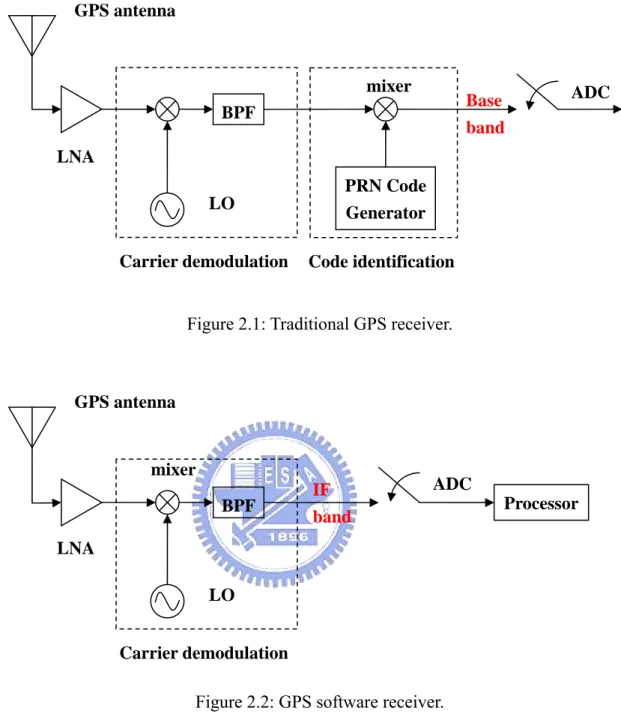
(18) Chapter 2 Global Positioning System As we know that baseband signal processing can achieve high-speed signal processing by means of dedicated hardware and software. By using specially-designed algorithm, we can acquire and track the satellite signals of GPS, obtain 50 bps of the navigation information and provide the estimation of C / A code and carrier, and then get a virtual distance. A baseband signal processing part includes numerical controlled oscillator (NCO), correlators and digital signal processors. In this chapter, we will offer an overview of GPS receiver first. Then, we focus on the discussion of the software receiver technique referred to [2]-[7]. Finally, we exploit the receiving algorithm for GPS software system to acquire and track satellite signals. The result of the acquired parameters and the tracking performance will be presented.. 2.1. GPS receiver. The GPS receiver is shown in Figure 2.1. In traditional GPS receivers, acquisition and tracking of signal are realized with hardware approach. Since the baseband signal processing is digital, acquisition and tracking can naturally be a pure software implementation. In this way, the receiver structure can be much simplified.. -5-.

(19) GPS antenna. mixer. Base band. BPF. ADC. LNA PRN Code Generator. LO Carrier demodulation. Code identification. Figure 2.1: Traditional GPS receiver.. GPS antenna. mixer BPF. IF band. ADC Processor. LNA LO Carrier demodulation. Figure 2.2: GPS software receiver.. The modern tendency of GPS receiver design is to use the concept of software defined receiver (SDR), which makes the position of analog-to-digital converter (ADC) as close to the antenna as possible. It can reduce the detrimental effects of temperature and aging in analog components. Moreover, apparent advantages including the flexibility of multiple navigation system and reprogrammable solution are afforded by software signal processing.. -6-.

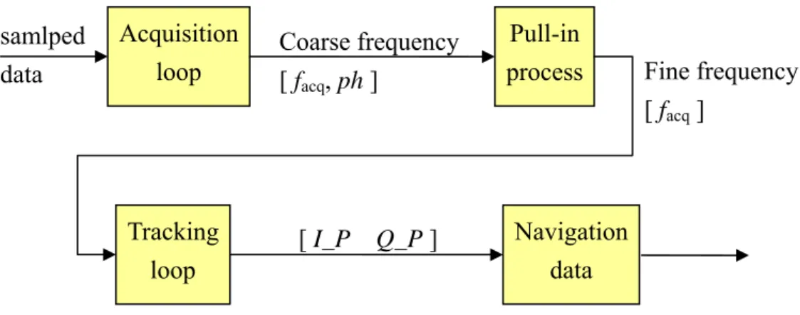
(20) Figure 2.2 shows the block diagram of GPS software receiver. The purpose of signal processing in Figure 2.2 is to remove possible disturbing signals by filtering, amplify signal to an acceptable level, and down-sample signal to a selected intermediate frequency (IF). Since the IF of 15.42 MHz and the sampling frequency (fs) of 4.096 MHz are chosen in our study, the center frequency of the signal is 11.324 MHz (=IF-fs), denoted as IFnom. (The detailed treatment of the antenna, the RF chain, and the digitizers can be found in Chapter 6 of Ref. [2].) As long as the signal is digitized and stored in memory, we can use the powerful DSP to replace some of the hardware features. The so-called software GPS is to use software to achieve the acquisition and tracking of satellite signals. In this thesis, we divide the software processor into four function blocks as Figure 2.3 and will discuss detailed treatment of each block in the following sections. A software receiver can process data in batches. One simple example is the application of the FFT to a batch of data [4]. As will be shown later, such processing allows for more robust signal acquisition.. samlped data. Acquisition loop. Coarse frequency [ facq, ph ]. Tracking loop. [ I_P Q_P ]. Pull-in process. Fine frequency [ facq ]. Navigation data. Figure 2.3: Software processor in GPS receiver.. -7-.

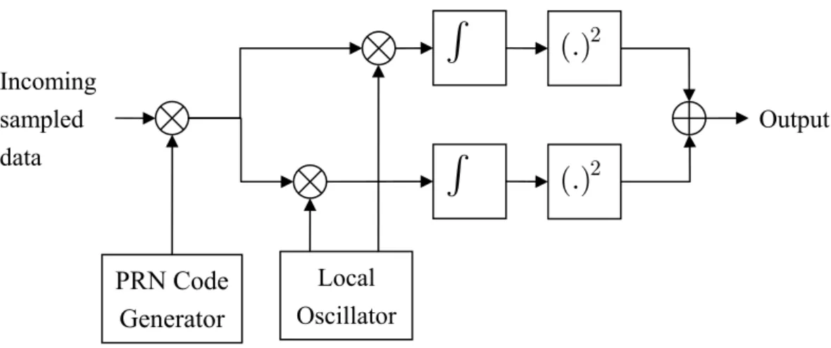
(21) GPS signals are all contained in a set of sampled data and we can search for different satellites by examining the sampled data. If the processor speed is quick enough to deal with different code phase matching, the relevant results may be faster than finding in time division by hardware. Under this condition, the processing speed and cost (size of the memory) determines the latency allowable for the signal processing software.. 2.2. Acquisition of GPS C/A Code signals. The primary purpose of acquisition is to determine what visual satellite is. In the acquisition loop, two important parameters must be obtained and passed to the next function block. One is the coarse value of carrier frequency and the other is the phase shift of PRN code. In general, acquisition algorithms have the following two approaches: time domain correlation and frequency domain correlation. Time domain correlation algorithms can be divided into the linear search and data in a bank. Frequency domain algorithms can be divided into the full FFT treatment and half-FFT treatment [2]. The block diagram of conventional acquisition method is shown in Figure 2.4. The information needed for acquisition is the sampled data. Fist of all, we need to decide the operation data length. In practice, the maximum data length used for acquisition is limited to 10ms because [2]: 1.. There could be a navigation data transition since the navigation data is 20 ms or 20 C/A code long.. 2.. The Doppler effect on the C/A code.. To simplify the experimentation, it’s sensible to operate on 1ms block of data corresponding to the length of a complete C/A code. If the signal is digitized at 4.096 MHz, 1 ms data contains 4096 data points. -8-.

(22) ∫ Incoming sampled data. (.)2 Output. ∫ PRN Code Generator. (.)2. Local Oscillator. Figure 2.4: Block diagram of acquisition in time domain.. Assuming that the received signal s(t) is composed of several visual satellite signals, we determine whether the signal is belonging to a particular satellite by comparing with 32 possible satellite PRN codes defined for satellite identification numbers. When we acquire space vehicle number (SV), s(t) must multiply together with the digitized C / A code which is generated by local PRN code of satellite SV. To find the right PRN code offset, that is, the beginning of C/A code, the receiver slides a replica of the code in time until maximum correlation occurs. The local PRN code can be expressed as. lsv,i = csv e j 2π fit ,. where csv is the C/A code of satellite SV and. fi. (2.1). is the carrier frequency. Once the. signal is de-spread to a continuous wave (cw) by a correct C/A code phase, the carrier frequency will be found. The 4096 real and imaginary values of the products by cw and local generated carrier are squared and added together, and the square root of this value represents the amplitude of the output frequency bin.. -9-.

(23) F_low. IFnom. Finc. F_high. Figure 2.5: Frequency bins needed for carrier frequency estimation.. Because the assumption of 1 ms pre-detection integration time, the frequency resolution denoted as Finc is 1 kHz, which is the inverse of the data length [2]. Besides, the acquisition method must search over a frequency range of ±5 kHz to cover all of the possible Doppler shift for low-speed vehicles in contrast with high-speed aircraft [2]. Under these conditions, we have to adjust 11 frequency bins, 5 for each side of IFnom, until maximum correlation is obtained. As a result, the total acquisition time is proportional to the product of the C/A circular shift time and the frequency bin number, that is, 45056 (4096×11). This process could be time consuming. In an effort to accelerate execution speed, D. J. R. Van Nee proposed a new fast GPS code acquisition technique using FFT [5]. It is convenient for us to implement the acquisition scheme of software systems based on FFT/IFFT. To begin with, we denote the N-points sampled data and the PRN code of satellite SV as s(n) and c(n), and then the circular correlation operation will be represented as. rsv,i (m) =. N −1. ∑ s ( n ) c ( n + m) .. (2.2). n =0. To translate the above equation in the discrete time domain to frequency domain by FFT, it results in. - 10 -.

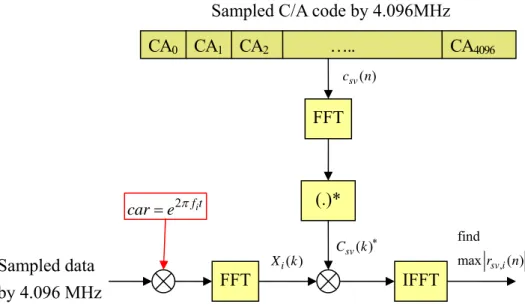
(24) Rsv,i (k ) = =. N −1 N −1. ∑ ∑ s(n)c(n + m)e− j 2π mk / N. m =0 n =0. N −1. ⎡ N −1. ⎤. n =0. ⎣ m =0. ⎦. ∑ s(n) ⎢ ∑ c(n + m)e− j 2π ( n+ m) k / N ⎥ e− j 2π (− n)k / N. (2.3). N −1. = C (k ) ∑ s(n)e j 2π nk / N = C (k ) S −1 (k ) = C −1 (k ) S (k ). n =0. where S −1 ( k ) and C −1 ( k ) are the inverse FFT (IFFT). If s(n) is real, s∗ ( n) = s ( n) where ∗ is the complex conjugate. Hence the correlation will be obtained from IFFT as below [6]:. rsv,i (m) = F −1 ( Rsv,i (k )) = F −1 (C (k ) S ∗ (k )) = F −1 (C ∗ (k ) S (k )) .. (2.4). It is easy to derive the above results and the proofs of them are ignored. From above properties, it is obvious that the circular correlation and FFT/IFFT is necessary if the frequency domain acquisition is used. The block diagram of frequency domain acquisition is shown in Figure 2.6. Before multiplied by the locally generated C / A code, the signal must be multiplied by the local carrier frequency as depicted in Figure 2.5 to remove the Doppler shift. For each frequency bin the following procedures are required: 1.. Complex multiply 1ms input data s ( n) with the one-bit quantized carrier point by point and transform the result into frequency domain as X i (k ) .. 2.. Generate the local code of satellite SV, csv ( n) which is sampled at 4.096 MHz.. 3.. Perform FFT on csv ( n) and take the complex conjugate to obtain C sv ( k )* .. 4.. Multiply X i (k ) with C sv ( k )* point by point to result in Rsv ,i ( k ) . - 11 -.

(25) Sampled C/A code by 4.096MHz CA0 CA1 CA2. …... CA4096. csv ( n). FFT. (.)*. car = e 2π fit. Sampled data by 4.096 MHz. FFT. X i (k ). find. Csv (k )∗. IFFT. max rsv,i (n). Figure 2.6: A block diagram of acquisition using FFT.. 5.. Take an inverse complex FFT of Rsv ,i ( k ) into rsv ,i ( n) and get a two dimension matrix rsv,i (n) .. 6.. Finally, code phase is the nth location in circular shift of the local code that gives maximum correlation, max rsv,i (n) , and the carrier frequency is the corresponding ith frequency bin in 1 kHz resolution.. 2.2.1. Pull-in process. From the above discussion, considering the frequency resolution of 1 kHz, the coarse frequency acquired from acquisition is not enough for accurate tracking. To solve the problem, a “pull-in” process is implemented to get fine value of carrier frequency. First of all, the main purpose here is to reduce the frequency resolution from 1 kHz to 200 Hz. Furthermore, Figure 2.7 shows that there will exist ambiguous range between the accurate carrier frequency and the acquired frequency, f acq .. - 12 -.

(26) new. facq-1k. Finc. Ambiguous range facq. facq+1k. Figure 2.7: Ambiguous range of carrier frequency.. For that matter, we determine the fine carrier frequency by searching 7 candidate frequencies that ranges between f acq ± 200i Hz, i = 1, 2,3 . As the C/A code has been found and only a few of candidate frequencies need to be examined, the pull-in function is performed by the time-domain correlation as shown in Figure 2.4.. 2.3. Tracking GPS signals. In this section, conventional tracking technique is presented. The main objective of tracking is to enhance the precision for the coarse evaluation from acquisition, keep tracking the satellite signals varying over time. The accuracy of the PRN code phase shift will affect virtual distance evaluation. In order to strip off the C/A code and track the frequency/phase of input signal, it requires two tracking loops: the code loop and the carrier loop, as shown in Figure 2.8. We will introduce the tracking processing for these two loops.. - 13 -.

(27) Code loop MA early Carrier frequency. e/d select. ∑. late MA. prompt. Carrier loop. cw. output. LPF θ f (t ). NCO. LPF. arctan. 0. 90. LPF. Figure 2.8: Code and carrier tracking loops referred to [2].. A. Code tracking The code tracking enhances the accuracy of code phase obtained via acquisition by using the delay locked loop (DLL). The DLL generates three local PRN codes: a prompt code which is the locally generated C/A code with the beginning determined from acquisition process, an early code and a late code which are shifted early and late by approximately one-half chip, respectively. Digital baseband I / Q signals, i.e. carrier wipe-off data in Figure 2.9, will be multiplied by these three codes individually. After passing through the correlation operation, a moving average filter, and finally the square function as we can see in Figure 2.9, it may result in tree correlation value denoted by Early_corval, Prompt_corval and Late_corval.. - 14 -.

(28) MA (moving average filter). Carrier wipe-off data. ∫. ( )2. ∫. ( )2. (early / late) C/A code. Correlation value. Figure 2.9: Part of code tracking loop.. According to the correlation result, we adjust code phase to generate new prompt code by a code loop discriminator, where the factor is denoted as EL which can be expressed as:. EL =. Early_corval . Late_corval. (2.5). We define the following operations for different early-late select value via statistics simulations [3]: 1. When resulting EL<0.8, the new prompt code will be generated by shifting first point of original prompt code to the end. 2. If the discrimination EL is more than 1.5, the new prompt will be obtained by shifting end point of original prompt code to the head.. - 15 -.

(29) B. Carrier tracking The carrier tracking follows the carrier frequency and phase changed after acquisition by using phase locked loop (PLL). A block diagram for the Costas carrier loop implementation is in Figure 2.10. PLL generates local carrier signal and measure the phase error between local carrier and the incoming digitized signal. Finally and most importantly, the PLL will adjust locally generated frequency to match the phase/frequency of the input signal.. PRN code I (k ), Q (k ). Incoming signal. Phase discriminator. Loop filter. NCO carrier generator. Figure 2.10: Carrier tracking loop.. To build software for digitized data, the PLL should transfer into the discrete z-domain through bilinear transform as. 2 1 − z −1 s= , ts 1 + z −1. (2.6). where t s is the sampling interval given by 10 −3 . Usually, the second-order PLL is widely used in GPS receiver because it has better performance in steady-state error [2].. - 16 -.

(30) θi ( z ). ε ( z). ∑. Vc ( z ). k0. Vo ( z). F ( z). −. θ f ( z) N ( z). Figure 2.11: Z domain.. Therefore, the filter function shown in Figure 2.11 will be. F ( z) =. C1 + C2 − C1z −1 1− z. −1. =. V0 ( z ) V0 ( z ) = , Vc ( z ) k0 (θi ( z ) − θ f ( z )). where we denote θi ( z ) − θ f ( z ) as the phase estimate, ε ( z ) ,and. (2.7). V0 ( z ) as the filtered k0. phase, while C1 and C2 are constants and will be calculated later. On the other hand, direct digital frequency synthesizer (DDS), also named numerical controlled oscillator (NCO), will replace the voltage-controlled oscillator (VCO) in PLL and its transfer function can be defined as. N ( z) =. θ f ( z) V0 ( z ). =. k1z −1. 1 − z −1. .. (2.8). Consequently, we can obtain the filtered phase offset for NCO as follows:. θ f ( z ) = V0 ( z ). k1 z −1. 1 − z −1. - 17 -. =. V0 ( z ) k0 k1z −1 . k0 1 − z −1. (2.9).

(31) Besides, two factors play an important role in the dynamic performance of the tracking loop and must be specified in order to implement the tracking loops. Based on the dynamics as discussed in [7], we denote the damping factor and noise (loop) bandwidths by ζ and ωn while optimally flat response will be achieved by. ζ = 1/ 2. 0.7 and ωn =50 Hz, respectively. According to the noise bandwidth. approximation for the tracking loop, the corresponding natural frequency will be presented as. Bn =. 2ωn =94.5945945945946 . 1 (ζ + ) 4ζ. (2.10). Assuming the carrier loop gain k0 k1 to be 4π × 100 , then C1 and C2 in (2.7) can be found as. C1 =. 8ζωnts 1 = 9.8635 × 10-5 , 2 k0 k1 4 + 4ζωnts + (ωnts ). 4(ωnts ) 2 1 C2 = = 6.6645 ×10-6 . 2 k0 k1 4 + 4ζωnts + (ωnts ). (2.11). Since the operation is performed every millisecond (msec), the local C/A will be regenerated and the phase of the local carrier frequency will be adjusted to match the incoming signals as closely as possible. In this case, the acquisition algorithm could merely provide a rough estimate of the necessary parameters, and then the tracking loops could further update the information that would be utilized to keep following the input signals changed over time.. - 18 -.

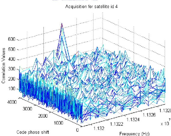
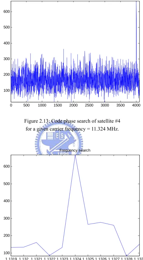
(32) 2.4. Computer simulations. In a software receiver, the acquisition algorithm described in Section2.3 could offer a rough estimate of the necessary parameters. The results for a particular GPS PRN code, SV #4 is presented by a 3-dimensional plot shown in Figure 2.12. Specifically, the collected experimental data is the real satellite signal received by NSPO. In this case, 4096 possible code phases are evaluated and 11 different frequencies are looked over for each code phase from 11.319 MHz to 11.329 MHz, separated by 1k Hz. The clear peak indicates PRN SV#4 is currently in use. The maximum correlation corresponds to the actual code phase of the 4079th sample and frequency offset of 11.324 MHz, as shown in Figure 2.13 and Figure 2.14, respectively.. Figure 2.12: Acquisition for satellite id #4.. - 19 -.

(33) Code phase search. 600. 500. 400. 300. 200. 100. 0. 500. 1000. 1500. 2000. 2500. 3000. 3500. 4000. Figure 2.13: Code phase search of satellite #4 for a given carrier frequency = 11.324 MHz.. Frequency search. 600. 500. 400. 300. 200. 100 1.1319 1.132 1.1321 1.1322 1.1323 1.1324 1.1325 1.1326 1.1327 1.1328 1.1329 7. x 10. Figure 2.14: Frequency search of 11 frequency components, in 1k Hz step for a given code phase.. - 20 -.

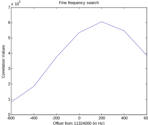
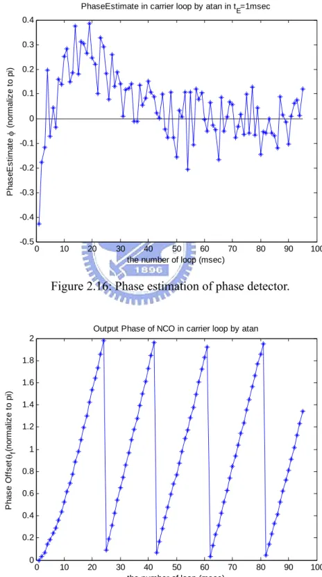
(34) 5. 7. Fine frequency search. x 10. 6. Correlation Values. 5. 4. 3. 2. 1. 0 -600. -400. -200 0 200 Offset from 11324000 (in Hz). 400. 600. Figure 2.15: Fine frequency search in 200Hz step in the pull-in process.. The second stage in processing the GPS signal is to pull in the carrier frequency. This is demonstrated in Section 4.2.2 that the real frequency is within f acq ± (1k / 2) , namely 11324000 ± 500 Hz. As shown in Figure 2.15, the maximum occurs at a frequency offset of 200Hz from the acquired frequency. In other words, we obtain a more accurate carrier frequency, 11.3242 MHz, after this processing. In the following, the general tracking implementation as described in Section 2.4 is performed. Here we concentrate on the phase component of carrier tracking loop. The simulation result for the filtered phase of NCO is presented in Figure 2.17. Compared with precise detection output of the phase detector shown in Figure 2.16, it is obvious that the phase angle of NCO changes little by little, which is based on previous estimated phase and detected phase after filtering by some coefficient according to (2.9).. - 21 -.

(35) Also note that the adjusted output phase of NCO continuously increases as time goes on, indicating that there is a slight phase error caused by the frequency mismatch between NCO and incoming carrier.. PhaseEstimate in carrier loop by atan in t E=1msec 0.4. PhaseEstimate φ (normalize to pi). 0.3 0.2 0.1 0 -0.1 -0.2 -0.3 -0.4 -0.5. 0. 10. 20. 30. 40 50 60 70 the number of loop (msec). 80. 90. 100. Figure 2.16: Phase estimation of phase detector.. Output Phase of NCO in carrier loop by atan 2 1.8. Phase Offset θf (normalize to pi). 1.6 1.4 1.2 1 0.8 0.6 0.4 0.2 0. 0. 10. 20. 30. 40 50 60 70 the number of loop (msec). 80. Figure 2.17: Adjusted phase output of NCO. - 22 -. 90. 100.

(36) Tracking: Correlation values for 4 -> 41 C/N(approx) 500 400 300. Amplitude. 200 100 0 -100 -200 -300 -400. 0. 10. 20. 30. 40. 50 60 time(ms). 70. 80. 90. 100. 90. 100. (a) In-phase. Tracking: Correlation values for 4 -> 41 C/N(approx) 300 250 200 150. Amplitude. 100 50 0 -50 -100 -150 -200. 0. 10. 20. 30. 40. 50 60 time(ms). 70. 80. (b) Quadrature-phase Figure 2.18: In-phase and quadrature Costas loop components.. - 23 -.

(37) Finally, if the detected phase is toward zero, that means the tracking loop is operating at the locked state, the in-phase component will contain the navigation data where 20 points express a data bit of 20 msec long as shown in Figure 2.18 (a). On the contrary, the quadrature-phase arm of the loop as Figure 2.18 (b) looks like noise.. 2.5. Summary. In global positioning systems, the software receiver is preferred to offer tremendous flexibility. It should be noted that in an effort to reduce acquisition time and provide more robust signal acquisition, the parallel search technique using FFT based on frequency domain acquisition is preferred. Two important acquisition parameters, the beginning of the C/A code period as well as the carrier frequency, will be used in the subsequent tracking loop. After pull-in process, we can obtain fine carrier frequency with resolution of 200 Hz. The tracking loop contains a code loop which enhances the code phase by DLL and the carrier loop which tracks the signal frequency/phase by PLL. However, from the simulation result, there is a transient period for tracking loops to lock the signal because of the mismatch between NCO and incoming signal. The result implies that we can have some improvement on the carrier tracking loop structure.. - 24 -.

(38) Chapter 3 Tracking System Improvement To improve the tracking performance, here we design a frequency offset pre-estimation for the NCO in PLL. The idea is using the first few data to estimate frequency offset so as to reduce the required lock time. That is, we propose to improve the PLL performance by modifying the initial tracking loop structure.. 3.1. Phase estimation. Figure 3.1 shows an approach widely-used in practice, which employs the arctangent method to detect signal phase.. s (t ). sgn[ s (kTs )]. Inphase(k ). ∑. I Phase estimation. sgn(sin 2π f acq kTs ). Quadrature(k ). ∑. Q. sgn(cos 2π f acq kTs ). NCO Figure 3.1: Conventional phase detection method.. - 25 -. θˆ.

(39) Consider a received signal s(t) given as. s (t ) = A sin(2π f c t + θ ) + n(t ) ,. (3.1). where A is the signal amplitude, f c is the down-converted carrier frequency, θ is the unknown phase and n(t) is the added Gaussian noise. In the figure, the signal s(t) is one-bit quantized at t = kTs , k = 0,1, 2,... , where Ts is the sampling period. A NCO is used to detect the signal phase. The NCO. generates two one-bit quantized local carriers:. I NCO = sgn(sin 2π f acq kTs ) ,. (3.2). QNCO = sgn(cos 2π f acq kTs ) .. (3.3). where f acq is the carrier frequency obtained from the pull-in process, and sgn( x) is the sign function which returns 1 if x ≥ 0 and -1 if x < 0 . However, the acquired frequency is not the same as the carrier frequency since the frequency resolution of pull-in process is limited to 200 Hz. As the accuracy of carrier frequency is of concern, the frequency of NCO is assumed to be unequal to the incoming carrier frequency and we denote the frequency offset as Δf . Accordingly, the incoming signal in (3.1) can be written as. s (t ) = sin(2π ( f acq + Δf )t + θ ) + n(t ) .. - 26 -. (3.4).

(40) Thus, the signal Inphase(k) is given as. Inphase( k ) = sgn[ s ( kTs )] ⋅ sgn[sin(2π f acq kTs )] .. (3.5). Nevertheless, as one-bit ADC is employed to detect the phase θ , only polarity of the sampled signal is available. Based on the definition of the polarity function, it is easy to have the following equality:. sgn( x) ⋅ sgn( y ) = sgn( x ⋅ y ) ,. (3.6). where x and y are arbitrary real numbers. Using the above property, we can reformulate (3.5) as. Inphase(k ) = sgn[ s (kTs ) ⋅ sin(2π f acq kTs )] A = sgn{ [cos φk − cos(ω 'kTs + θ )] + n(kTs ) ⋅ sin(2π f acq kTs )}, 2. where φk = 2πΔfkTs + θ is. the. phase. difference, ω ' = 2π (2 f acq + Δf ) is. (3.7). the. high-frequency terms. Similarly, the signal Quadrature(k) in Figure 3.1 can be expressed as. A Quadrature(k ) = sgn{ [sin φk − sin(ω 'kTs + θ )] + n(kTs ) ⋅ cos(2π f acq kTs )} . (3.8) 2. - 27 -.

(41) 3.1.1. Optimization in the analog domain. Suppose Tob is the given observation time interval which is 1msec because of the length of C/A code. Assuming Δf = 0 such that φk = θ . If all the signals are kept in the analog domain without quantization, then the I-channel and Q-channel outputs become. I ' = ∫0 ob. A A [cos θ − cos(ω 'kTs + θ )] ≈ cos θ , 2 2. (3.9). Q ' = ∫0 ob. A A [sin θ + sin(ω 'kTs + θ )] ≈ sin θ . 2 2. (3.10). T. T. where the contribution of high-frequency terms is neglected in the summation and noise is neglected. As I ' and Q ' are proportional to cos θ and sin θ , respectively, the optimum detection of carrier phase angle θ can be estimated with the arc-tangent (atan) or arc-tangent-2 (atan2) function that is popular in practical phase estimation for software receivers [3]:. ⎧ Q' π π a tan( ), - ≤θ ≤ . ⎪ ' ˆ θ =⎨ 2 2 I ⎪ ' ' ⎩ a tan 2(Q , I ) , - π ≤ θ ≤ π .. (3.11). As shown in Figure 3.2, the results of atan function are limited to the interval -. π 2. ≤θ ≤. π 2. while atan2 function is limited to -π ≤ θ ≤ π .. - 28 -.

(42) 1 atan2(Qps ,Ips ). 0.8. atan(Qps ,Ips ). Output error (normalize to pi). 0.6 0.4 0.2 0 -0.2 -0.4 -0.6 -0.8 -1 -1. -0.8. -0.6. -0.4 -0.2 0 0.2 0.4 True input error (normalize to pi). 0.6. 0.8. 1. Figure 3.2: Comparison of Costas PLL discriminators.. 3.1.2. Approximation with one-bit quantized software receiver. Since we employ one-bit ADC to detect the phase estimation in the software receiver, the summation process in digital domain is actually an approximation mimicking integration in the analog domain. Assuming K = Tob / Ts is the number of samples within Tob after ADC, that is, 4096 points from 1 msec data per operation. Hence the factors for phase detector, I and Q, in Figure 3.1 are obtained as. I=. K −1. ∑ Inphase(k ) ≈ cos θ ,. (3.12). k =0. Q=. K −1. ∑ Quadrature(k ) ≈ sin θ .. k =0. - 29 -. (3.13).

(43) Finally, the estimated phase can also be calculated with the arc-tangent-2 function and the results will be used in next section. Importantly, it should be noted that the estimated phase in discrete time will be deviated from the real one due to significant quantization error resulting from the one-bit quantization.. 3.2. Carrier fine frequency resolution. From the above discussion, we can obtain the phase estimation through the approximation while the phase of the samples within Tob is constant. But we understand the frequency offset Δf is a principal factor affecting lock time. In order to improve the tracking speed, an additional frequency estimation to provide an accurate initial guess is inserted into the PLL. Considering slow-varying vehicle or user, the frequency variation within each sampled data set is little and the following algorithm can work. To analyze the carrier phase of each data set, we can figure out an average phase estimation φî per 1 msec long data set and it corresponds to the phase angle of the middle data point in this data set, as shown in Figure 3.3. Since φk = 2πΔfkTs + θ , the average phase of the ith data set can be approximated as. φî = 2πΔf × (i − 0.5) × Tp + θ .. where T p is the time between processing ,i.e. T p = 1 msec .. - 30 -. (3.14).

(44) ith data set. 1 fs. φî. (i+1)th data set. Time between processing （Tp=1 msec）. φî +1. Figure 3.3: Phase angle from two consecutive data sets.. Δfˆ , θˆ. PRN code. φˆ1,φˆ2 ,L,φˆTE. I (k ), Q(k ). Incoming signal NCO carrier generator. Phase discriminator. Loop filter. when i ≦ TE. Figure 3.4: Frequency offset estimation using carrier tracking loop.. Assuming it takes TE time to get a frequency offset estimation. In other words, the tracking loop doesn’t work before TE time. Figure 3.4 shows the block diagram of the modified tracking loop where {φˆ1 , φˆ2 ,L , φˆTE } are obtained initially. Once {φî } from each data are obtained, the estimation of frequency offset Δf can be calculated easily via (3.14), which is determined by. Δfî =. Δφî , 2π ⋅ Tp. where Δφî = φî +1 − φî , i = 1,..., TE − 1 .. - 31 -. (3.15).

(45) 3.3. Resolving ambiguity in fine frequency measurement. It is noted that each phase estimation φî would be affected by noise. While the GPS has poor SNR, the noise will seriously affect the detection of phase. The calculation of frequency offset measurement has been presented in (3.15), here we introduce the limitation of (3.15) and design a reasonable frequency offset evaluation. Whereas the pull-in frequency resolution obtained from 1ms data is 200Hz, the maximum absolute value of the frequency offset must be smaller than but not less than 100 Hz. Therefore, the phase difference Δφˆ must be less than 2π Δf. max. T p = 0.2π.. Moreover, the possibility of a π phase shift between two data sets due to navigation data could happen at the same time. Let Δfˆ1 ,…, ΔfˆL denote the L rational frequency offset estimations sieved out from Δφˆ1 ,…, ΔφˆTE −1 with the limitation. These frequency offsets will be used to calculate the desired fine frequency offset, denoted as f offset . The desired frequency offset estimation is evaluated as below:. foffset = sign(Δfâv )⋅ | Δfâv | .. (3.16). The sign of f offset is determined as. L. sign(Δfâv ) = sign[ ∑ sign(Δfˆl )] , l =1. - 32 -. (3.17).

(46) and the value of f offset will be obtained by. | Δfâv |= average of Δfˆl ,ok ,. (3.18). where Δfl ,ok are those with the same sign as sign ( Δfâv ) in Δfˆ1 ,…, ΔfˆL . While we have got the frequency offset, the corresponding phase angle θ referred to (3.14) will be evaluate by. θˆ = φˆTE − 2π foffset ⋅ (TE − 0.5) ⋅ Tp .. (3.19). After we obtain the estimated frequency offset and phase, the output of NCO will be adjusted to I NCO = sgn(sin(ωnew kTs + θ f )) ,. (3.20). QNCO = sgn(cos(ωnew kTs + θ f )) ,. (3.21). where ωnew is equal to 2π ( f acq + f offset ) and θ f is the resultant value from (3.19). Figure 3.5 shows the frequency offset estimation approach on GPS in practice.. - 33 -.

(47) PRN code=1. φˆTE +1 ,…. Simulation. Loop filter. N Inphase(k ) Phase Quadrature(k ) discriminator. Incoming signal. ms≦TE Y. NCO carrier generator. facq Phasecorr=0. facq+foffset Phasecorr=θˆ. N. φˆ1, φˆ2 ,L , φˆTE. ms==TE. phase offset calculate. foffset. Y. Frequency offset discriminator. facq+foffset Phasecorr=F(ψ). Figure 3.5: Flowchart of carrier tracking in GPS.. Finally, in order to evaluate the accuracy of the proposed frequency offset approach, we define the frequency offset error as:. σ=. 1 N. N. ∑ ( foffset - Δf )2n. ,. (3.22). n =1. where N is the total number of test times which is equal to 3000 without special indication.. 3.4. Computer simulations. A. Estimation time (TE) In this Chapter, we adjust the initial frequency offset at the expense of the first TE msec. Hence the most important issue is how long we need to get acceptable - 34 -.

(48) fine frequency resolution with δf = -30Hz, θi = 0π by atan2 30 SNR=100 dB SNR=-10dB SNR=-14dB SNR=-17dB SNR=-20dB. Frequency Offset error (σ ). 25. 20. 15. 10. 5. 0. 0. 2. 4. 6. 8. 10 12 TE (msec). 14. 16. 18. 20. Figure 3.6: Frequency offset performance under different SNR.. f offset . From the simulation result in Figure 3.6, we see that the error is lower than 10. Hz if TE is greater than 6 msec, thus TE = 6 msec will be our choice.. B. Limitation bound In Figure 3.7 and Figure 3.8, we show different performances which employ different bounds for limitation such as Δφˆ ≤ 0.22π and Δφˆ ≤ 0.24π to find Δfˆl , l = 1,..., L that are used to calculate f offset . Comparing Figure 3.6 with Figure 3.7, it is. shown that the bound for Δφˆ ≤ 0.24π ( =2π ×120Hz ×1msec ) has better performance especially in high frequency offset region.. - 35 -.

(49) fine frequency resolution with TE = 6msec, θ = 0π by |δ φ |<=0.22π 20 SNR=100 dB SNR=0dB SNR=-10dB SNR=-17dB SNR=-20dB. 18. Frequency Offset error (σ ). 16 14 12 10 8 6 4 2 0 -100. -80. -60. -40. -20 0 20 f:real freq offset (Hz) δ. 40. 60. 80. 100. Figure 3.7: Frequency offset performance under different SNR for Δfl ≤ 110Hz .. fine frequency resolution with TE = 6msec, θ = 0π by |δ φ |<=0.24π 20 SNR=100 dB SNR=0dB SNR=-10dB SNR=-17dB SNR=-20dB. 18. Frequency Offset error (σ ). 16 14 12 10 8 6 4 2 0 -100. -80. -60. -40. -20. 0. 20. 40. 60. 80. 100. δf:real freq offset (Hz). Figure 3.8: Frequency offset performance under different SNR for Δfl ≤ 120Hz .. - 36 -.

(50) C. Frequency offset error under different SNR From above simulation results, we find a special result that the performance of frequency offset estimation under SNR=100 dB is worse than SNR=-10 dB in some initial frequency offset. This is shown in Figure 3.9, for example the error when SNR=100 dB could be larger than that of SNR=-10 dB at Δf =70 Hz. To verify the cause, we present the simulated frequency offset error at various SNR under analog processing, as shown in Figure 3.10. As we can see, the results coincide with our intuition, that high SNR implies lees error. Compared with analog processing, we consider the special result in Figure 3.9 is similar to “Dither” effect which is routinely used in processing of digital audio and video data: an intentionally applied noise can randomize quantization error and have better performance on the contrary, as detailed in [8].. fine frequency resolution with TE = 6 , θi = 0.6π by atan2 25 SNR=100dB SNR=0dB SNR=-10dB SNR=-20dB analog SNR=200dB. Frequency Offset error (σ ). 20. 15. 10. 5. 0 -100. -80. -60. -40. -20. 0 f(Hz) δ. 20. 40. 60. 80. 100. Figure 3.9: Frequency offset estimation performance under different SNR with N=100.. - 37 -.

(51) fine frequency resolution with TE = 6 , θ = 0.6π by atan2 analog process. Frequency Offset error (σ ). 15 SNR=100dB SNR=40dB SNR=35dB SNR=0dB SNR=-10dB SNR=-20dB. 10. 5. 0 -100. -80. -60. -40. -20. 0 f(Hz) δ. 20. 40. 60. 80. 100. Figure 3.10: Frequency offset estimation performance under analog process with N=100.. D. Adjust sampling frequency to obtain better performance As discussed in Section 2.1, we know that GPS has poor SNR from -14dB to -24dB, here we concentrate on the performance for SNR = -20 dB. Since the GPS is implemented with one-bit quantization, using higher sample rate can improve the frequency offset measurement. First, it is shown that the error will be reduced to half when sampling frequency is doubled in Figure 3.11. Figure 3.12 shows all possible Δf versus frequency offset error under different fs. Consequently, if the system has four times sampling frequency, the estimation error will be restricted within 10Hz.. - 38 -.

(52) fine frequency resolution with δf = -25Hz, θ = 0.6π by atan2 25 Fs=4.096 MHz 2Fs 4Fs. σ (standard deviation). 20. 15. 10. 5. 0. 0. 2. 4. 6. 8. 10 12 TE (msec). 14. 16. 18. 20. Figure 3.11: Frequency offset performance under different fs.. fine frequency resolution with SNR = -20dB, TE = 6msec, θi = 0.6π by atan2 20. Fs=4.096M Hz 2Fs 4Fs. 18. Frequency Offset error (σ ). 16 14 12 10 8 6 4 2 -100. -80. -60. -40. -20. 0. 20. 40. 60. 80. 100. δ f :real freq bias (Hz). Figure 3.12: Δf versus frequency offset error under different fs.. - 39 -.

(53) E. Carrier tracking loop implementation From the above simulation results, we implement the proposed scheme on carrier tracking loop. The frequency tracking performance for 50 Hz initial frequency offset and various phase shift θ are shown in Figure 3.13 (a)-(d). It is clear that our proposed approach can significantly reduce the required lock-in time. Although it has to waste 6 msec, lock is achieved much more rapidly with precise frequency and phase evaluation.. PLL[new] in carrier loop by atan2 with (SNR, δ f , θi )=( -20dB ,50Hz ,-0.6π) ,σ = 5.2823 0.3 no foffset pre-estimation Phase error Estimation (normalize to π). 0.2. TE=6. 0.1 0 -0.1 -0.2 -0.3 -0.4 -0.5 -0.6. 0. 10. 20. 30. 40 50 60 ith msec data. (a). - 40 -. 70. 80. 90. 100.

(54) PLL[new] in carrier loop by atan2 with (SNR, δ f , θi )=( -20dB ,50Hz ,-0.2π) ,σ = 3.7149 0.5 no foffset pre-estimation Phase error Estimation (normalize to π). 0.4. TE=6. 0.3 0.2 0.1 0 -0.1 -0.2 -0.3. 0. 10. 20. 30. 40 50 60 ith msec data. 70. 80. 90. 100. (b). PLL[new] in carrier loop by atan2 with (SNR, δ f , θi )=( -20dB ,50Hz ,0.2π) ,σ = 1.0749 0.8 no foffset pre-estimation. Phase error Estimation (normalize to π). 0.7. TE=6. 0.6 0.5 0.4 0.3 0.2 0.1 0 -0.1 -0.2. 0. 10. 20. 30. 40 50 60 ith msec data. (c). - 41 -. 70. 80. 90. 100.

(55) PLL[new] in carrier loop by atan2 with (SNR, δ f , θi )=( -20dB ,50Hz ,0.6π) ,σ = 4.2115 1 no foffset pre-estimation. Phase error Estimation (normalize to π). 0.8. TE=6. 0.6 0.4 0.2 0 -0.2 -0.4 -0.6 -0.8 -1. 0. 10. 20. 30. 40 50 60 ith msec data. 70. 80. 90. 100. (d) Figure 3.13: Resulting error signals for zero frequency initialization and 6 msec estimation time (50 Hz initial offset and various phase shift.). 3.5. Summary. In this chapter, we propose a frequency offset measurement for improving tracking performance. Being applied to the slow-varying cases, we derive phase detection algorithm to execute offset pre-estimation and update the initial condition. By means of frequency offset and phase shift pre-estimation, we can improve the tracking performance even in the low SNR region. As shown in this chapter, such processing allows for more rapid signal tracking. To cooperate with a suitable increase of sampling frequency, the carrier frequency was within 10 Hz in error in above simulation results. Thus the software-based finer resolution algorithm has been successfully validated.. - 42 -.

(56) Chapter 4 Virtual Carrier Table for One-Bit Quantized Software Receivers When we begin to implement our PLL, the NCO should be able to produce a sinusoid with variable frequency. There are many well-known methods for performing functional mapping from phase to sine amplitude such as ROM look-up, coarse/fine segmentation into multiple ROM’s, the Nicholas method, the use of Taylor series, CORDIC algorithm. Also, the comparison of the total compression ratio, the size of the memory, the worst case spur level, and additional circuits and their effect on distortion and trade-offs are investigated in detail [9]-[11]. Because the possible number of generated frequencies is large and computing sine values would require a prohibitive amount of computation and program complexity, a pre-built look-up table is usually a better alternative in GPS software receiver. In this chapter, an elementary description of table-lookup method for the conventional NCO will first be introduced. However, while we enhance the frequency resolution by the method in Chapter 3, it requires a large sine table. Unfortunately, large table means high volume memory and high cost. In place of table look-up method, we propose a different approach under one-bit quantization which uses an iterative computation algorithm. - 43 -.

(57) 4.1. Carrier generator. First, the common way to produce a table of discrete angle θ i and sin θi is introduced in [9]. Suppose a sine table stores N (usually a power of 2) samples from one cycle of the waveform, each sample can be expressed as. sin θi = sin(. 2π i ), i = 0,..., N − 1 , N. (4.1). which is the mapped discrete amplitude of the sine waves with discrete frequencies. ω = 2π / N . Thus we can pre-build a phase to sin amplitude table shown as Figure 4.1 where we use n bits to represent the truncated phase address and the word-length of the ROM is m bits. Then the size of the ROM required to store this sin table is 2n × m bits.. sin value (represented by m bits) Sin0 =sin(θ0) Sin1 =sin(θ1). Phase angle θi (n bits). Sin2 =sin(θ2). SinN-1 =sin(θN-1). Figure 4.1: The general sin table with full range of 2π.. To return the sine value of an angle by looking up the table, we need to determine the discrete phase angle expressed in radian (rad.) first. To simplify the interpolation problem, we usually select the “nearest phase angle” interpolation to approximate the in-between sine samples. It is obvious that the resolution of the values stored in the sine table determine the spectral purity of the conventional NCO. Nevertheless, while we enhance the accuracy of our frequency resolution in NCO from 200Hz to 20 Hz with the - 44 -.

(58) approach in Section 3.2, the sin table has to be pre-built with 10 times precision by brute force method. In other words, we will require (2 n × 10) × m bits memory to store the full sin table. Even though there is a well-known technique of compression to generate the ROM samples for the full range of 2π by only π/2 rad. of sine information and another additional logic necessary, the pre-built sin table look-up method seems to be inefficient.. 4.2. Virtual carrier table. From above description, the memory size is important for us to build the overall sin table that we need to evaluate the NCO output. However, since one-bit quantization is employed in the SDR, only the polarity of the carrier is of concern. In order to simply the carrier generator, we propose a universal approach for one-bit quantized carrier generator. The key feature of the virtual carrier table (VCT) is that we determine the NCO output value being either positive or negative from the relationship between the previous result and the variation of phase angle. Let the generated carrier table contain N. carriers, in which the carrier. frequencies are given as. f m = f 0 + m ⋅ fu. ,. m = 1, 2,...N ,. (4.2). where f 0 is a fixed frequency and fu is the minimum spacing between frequency bins. Assume sin 2π f mt is one of the carriers to be generated. In discrete system, t = k / f s , k=0,1,2,3, …, are the sampling instants of the one-bit quantized SDR of. concern while k is the discrete time index and f s is the sampling frequency. Thus the sampled signal of sin 2π f mt can be written in - 45 -.

(59) sin θ k = sin 2π. fm f + mfu k = sin 2π 0 k. fs fs. (4.3). Since the result of carrier generation is deeply affected by the variation of phase angle between two discrete time, now we attempt to find out the relationship between two phase angles, that is, θ k −1 and θ k at discrete time k − 1 and k , which in written as. θ k −1 = 2π. f 0 + mfu (k − 1) , fs. (4.4). θ k = 2π. f 0 + mfu k. fs. (4.5). From Equations (4.4) and (4.5), the relationship between changes of phase angle and system coefficients is obtained; the variation, Δθ , can be written in terms of the parameters ( f 0 , m, fu , f s ) as follows:. Δθ = 2π. 4.2.1. f 0 + mfu . fs. (4.6). Algorithm. Assume fu =. f0 and we choose the sampling frequency such that f s = q ⋅ f 0 . In h. general, q is a relatively small number while h is a big one. For example, if f 0 = 106 Hz , q = 4 and h = 10 4 , then fu = 102 Hz and f s = 4 × 106 Hz . Under these assumptions,. the phase angle of (4.3) can be expressed as. - 46 -.

(60) θ k = 2π. f0 mf 2π 2π mk . ⋅k + ⋅ k + 2π u k = fs fs q q h { 1 424 3 αk. (4.7). βk. In the case, we can partition θ k into two variables denoted as 1.. αk =. 2π 2π . ⋅ k is a fast-varying phase angle changing at a step of q q. 2.. βk =. 2π mk ⋅ is a slow-varying one since h is large. q h. We further analyze how and when the slow-varying factor affects the carrier generator. The variation would be classified into two categories, an integer plus an irreducible fraction, as be shown below:. mk remainder . = int + h h. (4.8). Furthermore, we define the following parameters:. ⎢ mk ⎥ mod q, bk ∈ (0,1,..., q − 1) , bk = ⎢ ⎣ h ⎥⎦ ck =. mk ⎢ mk ⎥ , − h ⎢⎣ h ⎥⎦. (4.9) (4.10). where ⎢⎣ x ⎥⎦ denotes the largest integer less than or equal to x. Based on the above definitions, Equation (4.7) can be written in. θk = α k + βk =. 2π 2π ⎢ mk ⎥ 2π 2π ⋅k + ⋅ (⎢ + ck ) = ⋅ ( k + bk ) + ⋅ ck . ⎥ q q ⎣ h ⎦ q q. - 47 -. (4.11).

(61) Form the above equation, it is obvious that the term k + bk will be the critical factor affecting the change of phase angle. For a given m, corresponding to a specific carrier frequency f m = f 0 + mfu , we can calculate the value of k , denoted as kmi , at which bk changes its value from bk = i − 1 to bk = i based on the definition of bk . Assume S (it will be discussed later) is the maximum size of the particular time index set where kmS is the reset point, the change of bk can be detected by determining k as follows:. bk = 0 → {1 → { 2 → ...(i − 1) → { i → ...( q − 1) → {0 → { 1 → ... → { j. km1 km 2. kmi. kmq. km ( q +1). (4.12). kmS. On the other hand, kmi can be evaluated easily from. ⎡h×i⎤ , for i = 1, 2,..., S , kmi = ⎢ ⎢ m ⎥⎥. (4.13). where ⎡⎢ x ⎥⎤ denotes the ceiling function, which returns the smallest integer not less than x, or, formally, ⎢⎡ x ⎤⎥ = min{n ∈ Z x ≤ n} . In practice, we can calculate the set ( km1 , km 2 ,...kmS ) for every possible m in (4.2) by simply computing (4.13) and store them in memory. This can be done easily before carrier generation is actually performed. When carrier generation for a particular frequency f = f o + mfu is required, the corresponding polarity of sin θ k is obtained as follows. In the beginning, let sign[sin θ k ] be the polarity function of sin θ k , defined as. - 48 -.

(62) sign[sin θ k ] = 1,. 0 ≤ θk < π ,. = −1, π ≤ θ k < 2π .. (4.14). Next, referring to θ k from Equation (4.11), a new integer denoted uk is now given as. uk = k + bk ,. (4.15). Under some manipulations from (4.12) and (4.15), hence we can derive the value of uk from uk −1 as. ⎧ u + 1, uk = ⎨ k −1 ⎩uk −1 + 2,. if k ≠ kmi if k = kmi , i = 1, 2,..., S .. (4.16). Therefore uk is generally expressed as. uk = uk −1 + x ,. (4.17). where x = 1 if k ≠ kmi and x = 2 if k = k mi . There is an important assumption that q in (4.11) must be an even number, given q=2p, where p is an integer. Then Equation (4.11) can be rewritten as. θk =. π p. ⋅ uk +. π p. ⋅ ck .. (4.18). In the following we shall consider the general case with p ≥ 2 while the special case of p = 1 will be treated later. The simple expressions are exploited to determine. - 49 -.

(63) the variant phase angle in order to obtain one-bit quantized result of carrier generator. To consider sign[sin θ k ] for 0 ≤ k < kmS in part A, B.. A. General case In the beginning, for the general case of p ≥ 2 , we define. vk = uk mod p .. (4.19). Moreover, from (4.17) and (4.19), we obtain the following relationship:. vk = uk mod p = (uk −1 + x) mod p = [(uk −1 mod p ) + x]mod p. (4.20). = [vk −1 + x]mod p.. Combining Equations (4.18) and (4.20), we just determine sign[sin θ k ] from sign[sin θ k −1 ] as. ⎧ sign[sin θ k −1 ] , if vk = vk −1 + x < p, sign[sin θ k ] = ⎨ ⎩ − sign[sin θ k −1 ] , otherwise.. (4.21). Therefore the polarity of sign[sin θ k ] can be easily determined if vk −1 and sign[sin θ k −1 ]. are given. Consequently, if the initial parameters v0 = 0. sign[sin θ 0 ] = 1 are given, vk. and. and sign[sin θ k ] , k = 1, 2,..., kmS − 1 , all can be. obtained via (4.20) and (4.21).. - 50 -.

(64) B. Special case On the other hand, for the special case of p=1, Equation (4.17) still holds and (4.18) becomes. θ k =π ⋅ uk + π ⋅ ck .. (4.22). If sign[sin θ k −1 ] is given, the polarity of sign[sin θ k ] is simply given as. ⎧ − sign[sin θ k −1 ] , if k ≠ kmi (that is uk = uk −1 + 1), sign[sin θ k ] = ⎨ ⎩ sign[sin θ k −1 ] , if k = kmi (that is uk = uk −1 + 2).. (4.23). Consequently, based on the proposed algorithm, we can generate all the virtual carrier tables for q = 2 p, p = 1, 2,3,.... C. Reset point Finally, we consider sign[sin θ k ] for k ≥ kmS . The particular reset time index kmS can be resolved with careful observation from Equations (4.8) and (4.10).. Obviously, when k = h, the parameter ck = 0 . Therefore the particular time index kmS = h should be the reset point while bk = m mod q and S = m at the same time.. In this way, the size of ( km1 , km 2 ,...kmS ) that we should calculate and store would be equal to m for every possible m. However, for a given m and h decided from a particular frequency f = f o + mfu , there may be a further simplification for the parameter size S. Assume gcd(m, h) is the greatest common divisor of m and h, Equations (4.8) can be rewritten as - 51 -.

(65) m ×k mk gcd( m, h) remainder . = = int + h h h gcd( m, h) gcd( m, h). (4.24). And then the reset condition will be changed to. ck = 0 , when k =. h = kmS . gcd(m, h). (4.25). At the same time,. bk =. m mod q . gcd(m, h). Consequently, the particular time index kmS = the maximum size of S, would be set as. (4.26). h should be the reset point and gcd(m, h). m for every m. gcd(m, h). As (4.20) and (4.21) still holds for k = kmS , we can obtain vkmS sign[sin θ kmS ] as before. Since bk = m. gcd(m, h). and. mod q at k = kmS , we can set vkmS. and sign[sin θ kmS ] as the initial condition for the new signal sequence, i.e. k = kmS → k = 0 , vkmS → v0 and sign[sin θ kmS ] → sign[sin θ 0 ] , and apply the same. algorithm to generate carrier table for k ≥ k mS . Accordingly, the carrier generation can be continuously generated without length constraint.. - 52 -.

(66) 4.2.2. System description. The proposed algorithm to generate virtual carrier table are implemented as follows (see Figure 4.2 and Figure 4.3). In the figure, sinVCTk corresponds to sign[sin θ k ] using VCT. The initial conditions are set as: k = 0 , v0 = 0 and sign[sin θ 0 ] = sign[sin 0] = 1 . The parameter set ( km1 , km 2 ,...kmS ) is pre-calculated and stored in the memory for every m. For. example, if q=4, h=104 and m=7 , then ( km1 , km 2 ,..., km 7 ) = (1429, 2858, 4286,...,10 4 ) . Based on the algorithm, the polarity of sin θ k , k>0, can be obtained for any carrier frequency f = f o + mfu .. - 53 -.

(67) Input (m,q,h). Initial parameters V0=1, kmindex=1 sinVCT0=1. k = k +1 Calculate (km1,…,kmi,…,kmS). k = kmi No. Yes. vk = vk −1 + 2 kmindex=+1. vk = vk −1 + 1 vk < p. Yes. No. sinVCTk=sinVCTk-1. sinVCTk= - sinVCTk-1. vk = vk − p. output. Reset kmindex=1. k = kmS. k = 0 , v0 = vkmS. Yes. sinVCT0 = sinVCTkmS No. Figure 4.2: Flowchart of VCT generator for p≧2.. Input (m,q,h). Initial parameters kmindex=1 sinVCT0=1. k = k +1 Calculate (km1,…,kmi,…,kmS). k = kmi No Yes. sinVCTk=sinVCTk-1. sinVCTk= - sinVCTk-1. kmindex=+1. output Reset. k = kmS No. Yes. k = 0 , kmindex=1 sinVCT0 = sinVCTkmS. Figure 4.3: Flowchart of VCT generator for p=1. - 54 -.

(68) 4.3. Computer simulations. As the derivation in Section 4.2.1, it is unnecessary to pre-store all the particular decision parameters ( km1 , km 2 ,...kmS ) for every possibly m. Instead, the parameters will be evaluated immediately via numerical calculation and stored in memory when the frequency and system parameters are decided. To test and verify the accuracy of the proposed virtual carrier table approach, we take some examples of frequencies and system parameters for simulation, shown in Table 4.1. In these cases, the carrier frequency of NCO is. f c = f 0 + mfu , where f 0 = 106 Hz,. fu =. f0. h. = 100 Hz,. f s = q × f 0 Hz.. S. ( km1 , km 2 ,...kmS ). 104. 3. (3334,6667,10000). 2. 10. 4. 7. (1429,2858,4286,5715,7143,8572,10000). 7. 4. 104. 7. (1429,2858,4286,5715,7143,8572,10000). 14. 4. 104. 7. (715,1429,2143,2858,3572,4286 5000). m. q. h. 3. 4. 7. Table 4.1: Frequency and system factors.. First, Figure 4.1 shows the errors vs. discrete time index k of proposed approach that are compared with the sign[sin θ k ] generated by Matlab programming, denoted sinp[k]. It is evident that the resulting carrier using VCT is not completely matched with the one by programming. To understand the cause of the error points, we examine the corresponding time index k of the error point and analyze the phase angel accordingly, as resulted in Table 4.2.. - 55 -.

(69) error of Virtual Carrier Table, where (m,q,h)=(3,4,10000) 2 1.5 1. error. 0.5 0 -0.5 -1 -1.5 -2. sinp[k]-sinVCT[k]. 0. 0.5. 1. 1.5. 2. 2.5 k. 3. 3.5. 4. 4.5. 5 5. x 10. Figure 4.4: The errors between programming and VCT vs. discrete time index k.. sin θ k in programming. k fs. k. θ k = 2π f c. 0. 0π. 0. 180000. 90027 π. +1.1824e-011. 360000. 180054 π. -2.3649e-011. 380000. 190057 π. +8.3170e-011. Table 4.2: The analysis of the corresponding phase angel at the error point for m=3, fc=1000300Hz, fs =4 MHz.. In Table 4.2, the first error point results from the different definition of initial condition ( θ = 0 ) that we assume sign(sin 0) = 1 and sign(sin 0) = 0 in Matlab programming. Moreover, the second row ( k = 180000, θ k = 90027π ) should be sin θ k = 0 , by definition. But a little inaccuracy leads to sin θ k = +1.1824e-011 in. programming. Similar results happen for k =360000 and k =380000. - 56 -.

(70) error of Virtual Carrier Table, where (f0,h)=(1M ,10k ) 22 m=3,q=4 m=7,q=2 m=7,q=4 m=14,q=4. 20. accumulated number of errors. 18 16 14 12 10 8 6 4 2 0. 0. 0.5. 1. 1.5. 2 k. 2.5. 3. 3.5 5. x 10. Figure 4.5: The accumulated number of errors vs. time index k for 4 simulation examples.. To illustrate the correctness of the proposed carrier generator, we present several simulation examples as shown in Figure 4.5. Within the total of 3.5 × 105 simulation points, the number of error points is less than 22 and all are due to numerical error in calculating multiple of π. Thus the validity of the proposed VCT is justified. In Figure 4.6, we show another simulation example when it is used for specific center frequency denoted f acq after fine search by pull-in function block and a tuned frequency offset denoted Δf. from tracking in Chapter 3. Considering that the. modified frequency estimation is under 10Hz and the minimum spacing between frequency bins, fu , is dominated by some definition in Section4.2.1. VCT could be implemented by assuming that the fixed frequency f 0 = f acq and Δf can be expressed as m × fu , where m is an integer and fu =. f0. - 57 -. h. . As an illustration, f0 = 11324200 Hz,.

(71) f s = q × f 0 Hz , h = 107 , so Δf = m × 1.13242 Hz. The proof of virtual carrier table is. shown in Figure 4.6. From the result, it can be proved that the simulation result is correct for all the time index k within k ≤ 105 .. m q h. S. ( km1 , km 2 ,...kmS ). 4. 2 107. 1 (2500000). 7. 2 107. 7 (1428572,2857143,4285715,5714286,7142858,8571429,10000000). 7. 4 107. 7 (1428572,2857143,4285715,5714286,7142858,8571429,10000000). Table 4.3: Frequency and system factors for f0=11324200 Hz, fu=1.13242 Hz.. error of Virtual Carrier Table, where (fo,h)=(11.3242M ,10M ) 2 m=4,q=2 m=7,q=2 m=7,q=4. 1.8. accumulation of errors. 1.6 1.4 1.2 1 0.8 0.6 0.4 0.2 0. 0. 1. 2. 3. 4. 5 k. 6. 7. 8. 9. 10 4. x 10. Figure 4.6: The accumulated number of errors vs. time index k for f0=11324200 Hz, fu=1.13242 Hz.. - 58 -.