運用最大概似估計及期望最大演算法以重建與切割微正子斷層掃描與
微陣列影像之統計應用
Statistical Applications of Maximized Likelihood Estimates with the
Expectation-Maximization Algorithms for Reconstruction and Segmentation
of MicroPET and Spotted Microarray Images
研 究 生:陳泰賓 Student:Tai Been Chen
指導教授:盧鴻興 Advisor:
Henry Horng-Shing Lu
國 立 交 通 大 學
統 計 學 研 究 所
博 士 論 文
A Thesis
Submitted to Institute of Statistics
National Chiao Tung University in Partial Fulfillment of the Requirements for the Degree of Ph. D in Statistics
March 2007
Hsinchu, Taiwan, Republic of China
運用最大概似估計及期望最大演算法以重建與切割微正子斷層掃描與微陣列影 像之統計應用 學生:陳泰賓 指導教授:盧鴻興
國立交通大學統計學研究所 博士班
摘
要
正子斷層掃描影像(PET)針對功能性疾病診斷提供非侵入式且可量化等資訊; 然而PET影像品質與使用的重建演算法有很高的相依性。屬疊代法之最大概似期 望最大法(MLEEM)正快速成為PET影像重建的標準方法。常見的MLEM演算法對 於隨機事件修正是採用二個Poisson分配相減(即: Prompt與delay資料相減),此方 法將失去Poisson分配的特性。我們將提出可行的演算法解決此一問題。利用聯 合Poisson分配(即聯合Prompt與delay)做隨機事件修正並同時重建PET影像,稱之 為PDEM演算法;不僅保持了Poisson分配特性而且不會增加估計隨機事件修正後 的變異。利用模擬、實驗假體以及實際老鼠等資料,採用變異係數和半高全寬值 比較FBP, OSEM以及PDEM之影像重建品質。經由PDEM所得的影像品質均優於 FBP或OSEM。 三維microPET影像能對體內基因反應之追蹤與辨認提供重要的訊息。為了能 調查或了解基因表現情形,發展低雜訊且高精確度的重建方法有其必要性。因採 用PDEM演算法重建影像接著將利用統計混合模型切割影像。在這研究中,模擬 與實際老鼠資料評估所提之方法,結果顯示是所提出的方法具有合理且正確性。 另一應用是對微陣列針狀基因影像之切割;該影像能提生物醫學之基因資 訊。在這一應用使用高斯混合模型以及無母數的核密度估計等方法用來切割雙色 微陣列針狀基因影像。 16 片雙色基因影像設計嵌入已知濃度之 spike spots、重 複 Spots 以及染劑互換等實驗,將用以驗證與評估所提方法之有效性與正確性; 結果顯示所提之方法不僅能有效切割 Spots 同時對 Spots 的估計具有高準確性。
Statistical Applications of Maximized Likelihood Estimates with the Expectation-Maximization Algorithms for Reconstruction and Segmentation of
MicroPET and Spotted Microarray Images
Student: Tai Been Chen Advisor:Henry Horng-Shing Lu
Institute of Statistics National Chiao Tung University
ABSTRACT
Positron emission tomography (PET) can provide in vivo, quantitative and functional information for the diagnosis of functional diseases; however, PET image quality is highly dependent on a reconstruction algorithm. Iterative algorithms, such as the maximum likelihood expectation-maximization (MLEM) algorithm, are rapidly becoming the standards for image reconstruction in emission tomography. The conventional MLEM algorithm utilized the Poisson model, which is no longer valid for delay-subtraction after random correction. This study was undertaken to overcome this problem. The MLEM algorithm is adopted and modified to reconstruct microPET images with random correction from the joint Poisson model of prompt and delay sinograms; this reconstruction method is called PDEM. The proposed joint Poisson model preserves Poisson properties without increasing the variances of estimates associated with random correction. The coefficients of variation (CV) and full width at half-maximum (FWHM) values were utilized to compare the quality of reconstructed microPET images of physical phantoms acquired by filtered backprojection (FBP), ordered subsets expectation-maximization (OSEM) and PDEM approaches. Experimental and simulated results demonstrated that the proposed PDEM method yielded better image quality results than the FBP and OSEM approaches.
The segmentation of 3D microPET image is one of the most important issues in tracing and recognizing the gene activity in vivo. In order to discover and recover the activity of gene expression, reconstruction techniques with higher precision and fewer artifacts are necessary. To improve the resolution on microPET images, the PDEM method is applied. In addition, the advanced statistical technique based on the mixture model is developed to segment the reconstructed images. In this study, the new proposed method is evaluated with simulation and empirical studies. The performance shows that the proposed method is promising in practice.
The segmentation of cDNA microarray spots is essential in analyzing the intensities of microarray images for biological and medical investigations. In this work, the nonparametric method of kernel density estimation is applied to segment two-channel cDNA microarray images. This approach successfully groups pixels into foreground and background. The segmentation performance of this model is tested and evaluated by sixteen microarrays. Specifically, spike genes with various levels of contents are spotted in a microarray to examine and evaluate the accuracy of the segmentation results. Duplicated design is implemented to evaluate the accuracy of the model. Swapped experiments of microarray dyes are also implemented. Results of this study demonstrate that this method can cluster pixels and estimate statistics regarding spots with high accuracy.
誌
謝
感謝指導老師盧鴻興教授對我的用心教誨、鼓勵與支持,才能使這本論文 順利完成!同時也感謝陽明大學陳志成教授與中研院統計所陳珍信教授等人對 研究資料提供與研究方法建議,讓本文能有進展。感謝交大統計所有老師的教 導;學長姐等人的研究素材與努力;對於我在交大統計求學期間都有著莫大的影 嚮與幫助。 太多人對我求學過程中有情有義;好友一嗚、駿逸、炳熏、棟鴻、紹志,以 及沒有登錄的諸位好友們!謝謝你們的鼓勵和打氣,使我得以完成這本論文;同 時亦感謝交大管科博士班羅偉給予我實質支持與建言。你們都是我生命中之貴 人。 感謝家人對我求學期間的百分百支持;父母兄弟妹給予我勇氣完成此一論 文。最後我要謝謝我妻子 雯玲 在我求學與研究期間,不止給我勇氣和鼓勵,亦 盡心盡力操持分擔家務同時照顧幼女亭妤;她總是默默付出且靜靜等待,始終對 我有信心!本書付印之前,正逢雯玲懷胎 8 個月。謝謝妳的付出與努力,我於此 刻以此書,表達我對妳的感恩與謝意。期望我們未來都能平安與健康! 陳泰賓 筆于風城 2007.04
Contents
中文摘要………...i 英文摘要………...ii 誌謝………...iii Contents………...iv Table Contents……….v Figure Contents………vi 1. Introduction ……….1 2. Methodologies ………..72.1 Reconstruction with Random Correction for MicroPET Images 2.2 Segmentation of 3D MicroPET Images 2.3 Segmentation of Microarray Images 3. Applications on MicroPET Images ...22
3.1 The MicroPET Scanner 3.2 Reconstruction with Random Correction 3.2.1 Simulation Study 3.2.2 Phantom Study 3.2.3 Real Mouse Study 3.3 Segmentation of 3D MicroPET Images 3.3.1 3D Images 3.3.2 Simulation Study 3.3.3 Real Mouse Study 4. Applications on Microarray Images ………42
4.1 The Spotted Microarray Images 4.2 Evaluation from Spike Genes 4.3 Evaluation from Duplicated Genes and Swapped Arrays 5. Discussion and Conclusion ………...51
6. Future Works ………55
7. Acknowledgements ………57
8. References ………..58
Table Contents
Table 2.3.4-1: One set of eight spike genes with target contents and ratios in real microarrays.
Table 2.3.4-2: Another set of eight spike genes with target contents and ratios in real microarrays.
Table 3.2.2-1: Average and standard deviation (in mm) of 28 FWHMs for horizontal and vertical line profiles measured for comparing the spatial resolutions of PDEM, OSEM and FBP. Those values are measured at the 31st slice.
Table 3.2.2-2: A circular ROI with a radius of 9 pixels to the center of the uniform phantom was utilized to compare noise levels between the PDEM, FBP and OSEM. Those values were measured at the 40th reconstructed slice.
Table 3.3.2-1: Comparisons of the clustering results by K-means and GMM in Fig. 3.3.2-1A.
Table 3.3.3-1: The FWHMs and SNRs of segmented results by GMM are better than those by K-means in Fig. 3.3.3-5.
Table 4.2-1: The comparisons of SSEs are obtained for different methods based on spike genes. Array 1s is that obtained by swapping the dyes of Array 1. Relative improvement is specified by (GenePix-Method)/GenePix as a percentage.
Table 4.2-2: The comparisons of SSREs are obtained for different methods based on spike genes.. Array 1s is that obtained by swapping the dyes of Array 1. Relative improvement is specified by (GenePix-Method)/GenePix as the percentage.
Table 4.3-1: Used spots excluding spike spots and bad spots in each array are listed and “x2” means two duplicates on every array.
Figure Contents
Fig. 2.2.1-1. An example shows the procedure to decide the number of clusters and initialized values in the EM algorithm of GMM. There are two peaks from the estimated densities of . Hence, the number of clusters in GMM will be two and initialized values will be computed from the above equations.
) ( ˆ y
f
Fig. 3.1-1: The microPET R4 scanner in Taipei Veterans General Hospital is displayed.
Fig. 3.1-2: Two images of microPET sinograms from physical experiments of six point sources are displayed. In every sonogram, the horizontal axis represents the ordering of line of responses (LORs) and the vertical axis represents different angles from 0 degree to 180 degree. The pixel intensity in the sinogram records total gamma rays detected in a scanning time window.
Fig. 3.1-3: The above data matrices are used for reconstruction by the PDEM and segmentation by the GMM.
Fig. 3.1-4 The above data matrices are used for reconstruction by the FBP and OSEM with random pre-correction.
Fig. 3.2.1-1. The modified Shepp-Logan head image was used for simulation studies. The line profiles of PDEM were less noisy than those of FBP and OSEM. The PDEM technique reconstructed better images than the FBP and OSEM did with 5%, 10% and 30% random noise. All images were rescaled using their own maximum values.
Fig. 3.2.2-1. The 31st slice of the 28 line-source phantom reconstructed using the three methods are displayed. Both FBP and OSEM are reconstruction methods built into the microPET R4 system. All images were rescaled using their own maximum values. The images are shown in the rectangular window. Table 3.2.2-1 presents the comparisons of their FWHMs.
Fig. 3.2.2-2. The reconstructed 40th slice from a uniform phantom was used to investigate noise level generated by the three approaches. The white line indicates the position of the investigated line profile. All images were rescaled using their own maximum values. The images are shown in the rectangular window with enlarged central parts. Table 3.2.2-2 presents the comparisons of their CVs.
Fig. 3.2.3-1: Sagittal (top) and coronal (middle) images of the first mouse image reconstructed by PDEM (left), FBP (middle) and OSEM (right). The images reconstructed by PDEM have less noise than those reconstructed using FBP and OSEM with comparison by line profiles. The images are shown in the rectangular window with enlarged central parts.
Fig. 3.2.3-2. Coronal and sagittal images of the second mouse image reconstructed using PDEM (left), FBP (middle) and OSEM (right). The images reconstructed by PDEM have less noise than those reconstructed by FBP and OSEM, as shown in the respective line profile near the heart. The images are shown in the rectangular window with enlarged central parts.
Fig. 3.3.1-1. The flow chart of 3D segmentation is plotted.
Figure 3.3.1-2: 3D microPET images for 63 slices are illustrated. Every image has the pixels size of 128 by 128.
Fig. 3.3.2-1. A) Simulation image of five clusters is displayed. B) Adding 50% noise into panel A. C) Clustering results using GMM. D) Kernel density curve using C with values of high and low peaks. Four peaks are identified on the density curve. Hence, the number of groups is set as four.
Fig. 3.3.2-2. Target ROIs are marked.
Fig. 3.3.2-3. The results of A) by K-means and B) by GMM clustering are shown.
Fig. 3.3.2-4. Simulated volume data including slice 1 and 2 are marked as A and B. C and D are reconstructed images after added 50% noise ratio to A and B. E and F are segmented results without slice normalization. G and H are segmented results with slice normalization. I is the estimated kernel density curve of simulated volume data after slice normalization.
Fig.3.3.3-1. The estimated kernel density curve using the rat volume data of 10 slices is shown with values of high and low peaks. There are four peaks. Hence, the number of groups is set as four. Values of peaks are applied to compute the starting values in EM algorithm.
Fig. 3.3.3-2. The reconstructed rat images are shown from the 51st (top-left) to the 60th (bottom -right) slice.
Fig. 3.3.3-3. The results of segmentation by the GMM are shown from the 51st (top-left) to the 60th (bottom -right) slice.
Fig. 3.3.3-4. The results of segmentation by the K-means are shown from the 51st (top-left) to the 60th (bottom -right) slice.
Fig. 3.3.3-5. The horizontal line profile of the 60th slice of Fig. 3.3.3-2 is shown with FWHMs. The FWHMs of region 1, 2, 3 and 4 are 3.75, 3.40, 4.14 and 4.45 pixels respectively. The top part shows the location of this line profile in the MLEM reconstruction image and the segmentation by GMM and K-means.
Fig. 4.1-1: An example of microarray image with 32 blocks, 22 columns and 22 rows. One block is enlarged and eight spike genes are numbered.
Fig. 4.1-2: Typical segmentation of two spot images by the irregular segmentation method of GenePix 6.0. Parts a) and b) present the original images of Cy5 and Cy3 dyes. Parts c) and d) present the segmented region on the images of Cy5 and Cy3 dyes.
Fig. 4.1-3: Two estimated density curves for spot of Cy5 (a) and Cy3 (b) dyes. Both Cy3 and Cy5 images have two intensity distributions for background and foreground pixels. The local minimum is used to be cutting point for segmenting spot pixels.
Fig. 4.3-1: Top row shows four methods to evaluate duplicated spots for 3rd (red) and swapped 3rd (blue) arrays. The x-axis and y-axis represent average and difference between duplicated spots. Bottom row shows four methods to evaluate swapped arrays (3rd, 3rd s). The x-axis and y-axis represent summation and difference between swapped arrays.
Figure 4.3-2 shows the concordance correlation coefficients, Pearson’s correlations and standard deviations between replicates gene expression of sixteen arrays and eight swapped arrays.
Fig. 4.3-2: Top and down figure are concordance correlations, Pearson’s correlations and standard deviations between duplicated spots of sixteen arrays and between swapped arrays of eight arrays using the GKDE, KDE, GMM and GenePix 6.
Fig. B-1: The illustration of HWHM is shown.
1. Introduction
The techniques of microPET and microarray are two of the most powerful
modalities in the study of molecular gene therapy and gene expression profiles in this
century.
The high spatial resolution and sensitivity of microPET make it an ideal modality
for in vivo gene imaging. Those images can be employed to monitor the effects of
gene therapy inside animal bodies. Recent study [1] shows that the technique of
microPET has been developed to trace the gene expression in vivo. Hence, it is very
important to enhance the reconstruction and analysis techniques with better precision
and fewer artifacts so that the genuine gene expression inside biological objects can
be recovered. High-quality image reconstruction is essential in establishing a solid
basis for quantitative study of microPET images [2-3].
The conventional methods built-in microPET software (microPET manager V1.6.4),
filter backpropagation (FBP) [4] and ordered subsets expectation-maximization
approach (OSEM) [5], are used to reconstruct microPET images after applying the
Fourier rebinning (FORE) algorithm [6] and random pre-correction. However, the
FBP is unable to model the randomness of PET. As the FBP was developed for
transmission tomography, it is not accurate when applied to emission tomography
image is typically noisy and inaccurate. Meanwhile, the OSEM can reconstruct more
accurate images than the FBP does, but it is basically driven from the inaccurate
Poisson model using random pre-correction (that is, applying subtraction on two
random variables from two independent Poisson distributions).
On the contrary, iterative algorithms, such as the maximum likelihood
expectation-maximization (MLEM) algorithm, are rapidly becoming the standards for
image reconstruction in emission tomography. The MLEM reconstruction and related
improvements have also been reported in literature [7-10, 14, 16-17, 21-24].
Statistical analysis that supports positron emission tomography (PET) has been
discussed as well [9]. The MLEM approach can model randomness in emission
tomography with the asymptotic efficiency by applying the row operation and
monotonic convergence using the EM algorithm. Furthermore, the EM algorithm can
be parallelizable for 3D PET image reconstruction [10].
The generation of quantitative PET images requires that the effects of random
coincidences and coincidence efficiencies are corrected [11-12]. One random
correction approach applies single count rates to a prompt sinogram [13]. This
approach is generally based on geometric and physical characteristics. However, this
approach makes many assumptions for approximations that can decrease the accuracy
delay sinograms. An alternate approach applies random pre-correction to sinograms
by subtracting the delay sinogram from a prompt sinogram before the processing of
images reconstruction. The random pre-correction using various approximations has
been applied to correct random (or accidental) coincidental events [14-15]. Different
methods have been developed to approximate the distribution of random
pre-correction [16-18]. However, random pre-correction increases the variances of
estimates [17, 19]. Since the distribution of random pre-correction is no longer
Poisson-distributed, the shifted Poisson methods and saddle-point (SD) approximation
have been generated to enhance approximation [20]. This study proposes a joint
Poisson model of prompt and delay sinograms for random correction with the MLEM
reconstruction without using approximations nor increasing variances. This approach
is named PDEM. Simulations, physical phantoms and real Mouse studies of the
PDEM method using the microPET R4 system were performed. This study analyzed
and assessed the reconstruction of 2D data obtained from 3D sinograms after applying
the FORE method to verify the proposed approach. The PDEM method can also be
utilized in future studies reconstructing 3D images.
Once microPET images have been reconstructed using PDEM, the next step is to
segment those regions of interest (ROI) from the reconstructed images. The FBP
Wong et al. [26-28] used the method of FBP reconstruction and K-means clustering
with Akaike information criterion (AIC) [25] to segment PET images. However, the
FBP method is not accurate for reconstructing microPET images. Hence, the PDEM is
applied to reconstruct microPET images more accurately instead of the FBP in this
study. Due to the variability of variances among different segments of microPET
images, we will consider the Gaussian mixture model (GMM) instead of K-means
clustering [28-30]. Furthermore, the numbers of cluster and their initialized values
used in GMM are determined by the kernel density estimation (KDE).
Similar methods can be adapt to segment spotted microarray images. The
microarray is a high throughput technique for exploring the expression profiles for
thousands of genes during the studies of genomics in biology and medicine. Although
high-density oligonucleotide arrays are currently available, custom-made or spotted
cDNA microarrays have also been used, because of their favorable cost, ease of
preparation and ease of analysis in the design of co-hybridization experiments [32].
Studies of the functionality of genes in this new era of post-genomics are important
[33]. Analyzing the microarray images with high accuracy is essential to measure the
gene expression profiles. Advanced analysis for selecting significant genes, clustering,
classification, and network reconstruction of gene expression profiles can proceed on
The cDNA images, in general, tend to be very noisy. Therefore, various approaches
have been proposed to improve the calibration of scanning efficiencies, the alignment
and detection of spotting errors, the denoising of background noise from images, the
marking of dust, gridding, moving, hybridization and other artifacts [34, 36-37].
Different methods have been proposed for segmenting cDNA microarray images in
literature. Markov Random Field (MRF) modeling has been proposed to segment
spots in microarray images [32]. This MRF-based approach relies on the prior
assumption of class labeling of all pixels [38] and it has a high computational cost.
The alternative approach of region-growing approach relies on the selection of initial
seeds that influence its performance [39]. the other approach of Gaussian mixture
model (GMM) generally assumed normality when it is applied to this segmentation
problem [40]. Accordingly, this study is motivated by the need to investigate the
segmentation of cDNA microarray images using the nonparametric method of kernel
density estimation (KDE) that does not require the assumption of normality.
In this investigation, the KDE is utilized to classify pixels in a spot into background
and foreground that use the estimated density to find the cut-off value. Meanwhile,
the approach of initial segmentation using GMM and fine tuning using KDE is
proposed to detect feasible boundary between foreground and background in spots.
conducted on real microarray data that involve 256 spike genes with known contents.
The segmentation results obtained by the KDE are compared with those obtained
using the adaptive irregular segmentation method used in the current version of
GenePix Pro software 6.0 (at http://www.moleculardevices.com/pages/software/ gn_genepix_pro.html, with the accompanying User’s Manual).
Microarrays with various sources and experimental designs are needed to monitor
the variations of gene expressions. Spike spots of the corresponding spike mRNAs
with a range of concentrations are used to monitor the variability of fluorescence
intensities and determine the consistency of hybridization among arrays. The spike
spots also reveal the variations of pins in an array. Duplicated spots within each array
are used to assay the hybridization process of the arrays. Swapped experiments are
also used to assay the labeling efficiency of Cy3 and Cy5 fluorescence dyes.
In this application, real microarray images with (1) spike spots with various ratios
of Cy5 to Cy3 intensities, (2) duplicated spots in an array and (3) the swapping of
microarray experiments, are applied to evaluate the performance and accuracy of the
2. Methodologies
This chapter begins with the introduction of algorithms and methods used for
reconstruction and segmentation accordingly. Section 2.1 introduces the proposed
PDEM approach to reconstruct microPET images with random correction. Section 2.2
shows the GMM applied to segment 3D microPET images by the automatic
determination of the number of clusters and initialized values by KDE. Section 2.3
presents the GKDE approach that is applied to segment spotted cDNA microarrays.
2.1 Reconstruction with Random Correction for MicroPET Images
A new approach is proposed to reconstruct microPET images with random
correction by the joint Poisson model of prompt and delay sinograms. We will assume
that the data in prompt and delay sinograms follow two independent Poisson
distributions that are labeled as (1) and (2).
)), ( ( ~ ) ( * * d Poisson d np
λ
(1) )), ( ( ~ ) ( * * d Poisson d ndλ
r (2)where *(d) *(d) *(d) P(b,d) (b) *(d), b indicates the b r b t r t λ λ λ λ λ = + =
∑
+ th pixel of atarget image with size B = 128x128 in which b=1,2,…,B, and d indicates the dth LOR
with total numbers D = 96x84 in which d=1,2,…,D. The term n*p(d) is the number of coincidental events in the prompt sinogram at the dth projection line of response
(LOR), which is formed by two detectors with the Poisson mean,λ*(d);
) (
* d
number of random coincidental events in the delay sinogram with the Poisson
mean *(d); P(b,d) is the system probability matrix from the b r
λ th pixel to the dth LOR.
Parameters of λt(b) and ( )
* d
r
λ are unknown and must be estimated. Parameter )
(b
t
λ represents the intensities of true coincidental events. Appendix (A3) lists the log-likelihood of observed data in the prompt and delay sinograms. Since the
maximum likelihood estimate (MLE) is difficult to find by maximizing Eqs. (1) and
(2) numerically, the EM algorithm [30-31] can be utilized (as the details in Appendix).
Equations (3) and (4) are the ith iteration steps of the PDEM.
∑
∑
∑
= − = − = − + = D d i r B b i t p D d i t i t d b d b p d b p d n d b P b b 1 * 1 1 ' 1 * 1 1 ) ( ) ' ( ) ,' ( ) , ( ) ( ) , ( ) ( ) ( λ λ λ λ , (3) ⎥ ⎥ ⎥ ⎥ ⎦ ⎤ ⎢ ⎢ ⎢ ⎢ ⎣ ⎡ + + = − = − −∑
( ,' ) ( ') ( ) ( ) ) ( ) ( 2 1 ) ( * 1 * 1 ' 1 1 * * * n d d b d b p d d n d d i r B b i t i r p i r λ λ λ λ , (4)where i=1,2,……I, is the number of iterations.
The MLEM algorithm of joint the prompt and delay sinograms is described as
follows and such a scheme is called PDEM reconstruction.
Algorithm for PDEM reconstruction:
Step 1: Set the initial parameters (i=0) using the FBP, the method of moments
estimate (MME) or alternative approaches.
the parameters by applying Eqs. (3) and (4).
Step 3: If (that is, the difference of
log-likelihoods among new and old estimates is smaller than for a tolerance
level), then the iteration is terminated; otherwise, go to Step 2. tolerance d b l d b l i r i t in i r i t in( ( ), ( ))− ( − ( ), − ( ))< 1 * 1 * λ λ λ λ
This method preserves Poisson properties and update estimates iteratively. In this
study, P(b,d) was computed from LORs and the locations of pixels based on the
geometric characteristics of the microPET R4, including number of detectors, image
size, field of view (FOV), ring diameter, and number of angular views. The matrix
size of one slice is 96×84. There are 96 angular views and 84 LORs for each angular
view during image scanning. Furthermore, each P(b,d) can be identified from its
detector pairs of LOR and image pixel location. Therefore, the PDEM reconstructs the
sinogram after the step that sinograms are rebinned by the FORE approach in the
microPET system.
2.2 Segmentation of 3D MicroPET Images
This section briefly introduces the segmentation algorithm of 3D microPET image.
Several pre-processing steps are used before the GMM algorithm is applied to
segment 3D microPET image. The number of clusters to be used in GMM and the
nonparametric method of KDE is employed to estimate the density curve of image
intensities. The numbers of cluster (k) can be determined by searching the number of
local maximum points from the estimated density curve. In addition, the initialized
values of parameters for the normal distributions in k clusters can be determined from
the data consequently.
2.2.1 Determination of the Cluster Number for GMM
The kernel density estimation (KDE) [41] will be applied to determine the
number of clusters used in GMM. From the estimated density curve, those high and
low peaks could be used to estimate the means and standard deviations of Gaussian
distributions in clusters. It is based on the empirical rule that the range of μ ±3σ
covers most of observations from a normal distribution. Hence, the initialized values
of GMM are determined by applying this empirical rule (as illustrated in Fig. 2.2.1-1).
This approach can automatically decide the cluster number and starting values of
parameters in the EM algorithm of GMM. This is a simple and computation
Fig. 2.2.1-1. An example shows the procedure to decide the number of clusters and initialized values in the EM algorithm of GMM. There are two peaks from the estimated densities of . Hence, the number of clusters in GMM will be two and initialized values will be computed from the above equations.
) ( ˆ y
f
Algorithm of KDE for Determining the Number of Clusters
A Gaussian kernel function is used to estimate the density of data as in Eq. (5),
, ) 2 / ) ( exp( 2 1 1 ) ( ˆ 1 2
∑
= − − = n i i j j h x y h n y f π (5)where xi is the ith sample, yj is the jth grid point, h is a bandwidth using in the Gaussian
kernel to estimate a probability density function, n is the sample size, and j = 1, 2, …,
128.
Step 1: Input dataX ={x1,x1,L,xn}.
Step 2: Find 128 grid points using equally spaced as Eq. (6):
. / )) ( ) ( ( ) (X j Max X Min X m Min yj = + − (6)
Step 3: Calculate the data-driven bandwidth for KDE as Eq. (7):
} 34 . 1 , { 9 . 0 −1/5 = Min Std IQR n h (7)
where Std is the standard deviation of X and IQR is the interquartile rang of X
[44].
Step 4: Calculate the KDE using Eq. (5).
Step 5: Determine the number of clusters by counting the number of local maximum.
standard deviations of Gaussian distributions in clusters like the illustration in Fig.
2.2.1-1.
2.2.2 Gaussian Mixture Model (GMM)
For the study of a set of 3D images from microPET, Ixyz represents the intensity at
the xyzth voxel. The range of the position xy in one slice has the size of 128x128 and
the number of slices z has the size of 10 in this study. Since the variance scale in
different segments of 3D images may be different, we consider Gaussian mixture
model with different parameters of means and variances in various clusters [28-29].
We will suppose that the image data Ixyz follow a mixture of K distributions with the
mixing probability
π
k such that∑
= = ≤ ≤ = K k k k k K 1 . , , 2 , 1 all for 1 0 and , 1 π L π (8)That is, the probability density function of Ixyz is
, ) ; ( ) ; ( 1
∑
= = Φ K k k xyz k k xyz f I I f π θ (9) where fk(Ixyz,θk) refers to the probability density function in the kth cluster withparameter θk. All parameters are collected to form a parameter vector
). ,..., , ,..., (π1 π K θ1 θK =
Φ The MLE of every parameter is usually difficult to
obtain directly by numerical methods. Alternatively, the EM algorithm can be applied
⎪⎩ ⎪ ⎨ ⎧ = otherwise. 0, on; distributi normal from comes if , 1 xyz th xyzk k I C (10)
Let Cxyz = (Cxyz1, …, CxyzK) denote the unobserved index vector and {Ixyz, Cxyz} form
the complete data for applying the EM algorithm. Given Cxyz, the conditional density
of Ixyz becomes .) ; ( ) | ( 1
∑
= = K k xyzk k k xyz k xyz xyz C C f I I f π θ (11)The EM algorithm finds MLE of parameters with the constraint of Eq. (8) by the
following iterative procedure:
, ) ; ( ) ; ( 1 ) ( ) ( ) ( ) (
∑
= = K j old j xyz j old j old k xyz k old k xyzk I f I fθ
π
θ
π
ω
(12)∑
= = N xyz xyzk new k N 1 ) ( 1ω
π
, (13) , ) ( 1 ) ( new k N xyz xyz xyzk new k N Iπ
ω
μ
⋅ ⋅ =∑
= (14).
)
(
) ( 1 2 ) ( ) ( 2 new k N xyz new k xyz xyzk new kN
I
π
μ
ω
σ
⋅
−
⋅
=
∑
= (15)The Gaussian distribution for the kth cluster is listed below,
. / ) ( 2 1 exp ) 2 ( ) , ; ( ) ; ( 2 2 2 1 2 ⎟ ⎠ ⎞ ⎜ ⎝ ⎛− − = = k k k k − k k k k x f x x f θ μ σ πσ μ σ (16)
EM Algorithm for GMM
Step 1: Set the initial parameters Φ (old).
Step 2: Update the parameters by using Eqs. (12) - (15).
Step 3: If lin(Φ(new) ) –lin (Φ(old)) < tolerance (that is, the difference of log-likelihoods
among new and old estimates is smaller than for a tolerance level), then the
iteration stops. Otherwise, go to Step 2 with the old values of parameters
replaced by the new values.
2.2.3 Slice Normalization
The intensity heterogeneity in slices of microPET images comes from the
differences in emission activities and reconstruction processes. The heterogeneity
between slices will affect the accuracy of the segmentation of 3D images. Hence, slice
normalization is needed before 3D segmentation to adjust image levels between slices.
We will use the slice normalization defined in Eq. (17),
z z z xyz new xyz
Min
Max
Min
I
a
I
−
−
=
, (17) where is the new intensity after slice normalization, is the originalintensity at xyz new xyz
I Ixyz
th voxel, is the minimum value of the z
z z
Min th slice, is the
maximum value of the z
Max
th slice, and a is a nonzero constant for the range of adjusted
2.3 Segmentation of Microarray Images
This section discusses three segmentation algorithms for spotted microarrays.
Empirical evaluation of the performance for segmentation methods will use different
criteria based on target ratios of spike genes, duplicate spots in a microarray image,
and swapped microarray images Cy3 and Cy5 dyes. In this study, the aim is to
segment pixels into foreground or background. Hence, there are two clusters used for
the segmentation of the pixel intensities in a spot. Besides the GMM with EM
algorithm, we will propose the KDE and GMM incorporated the KDE (GKDE) to
segment spotted microarray image in this study.
2.3.1 Kernel Density Estimation (KDE)
The KDE with automatic bandwidth selection [41] is used to estimate the density
function of pixel intensities for each spot. The Gaussian kernel function and 128 grid
points are used for the KDE for each spot as Eq. (5) in section 2.2.1. The details are
reported in the following algorithm.
Algorithm for Segmenting One Spot by KDE
Step 1: Input dataX ={x1,x1,L,xn}.
Step 2: Find 128 grid points that are equally spaced as Eq. (6).
Step 4: Calculate the KDE using Eq. (5).
Step 5: Search the cut-off point (CP) that is the first local minimum of the KDE at yj*
and let CP = yj*.
Step 6: Segment the pixelx into foreground ifi xi >CP, else into background.
2.3.2 Gaussian Mixture Model (GMM)
The GMM assumes that the distribution of foreground intensities is a Gaussian
distribution ( , 2) with mean 1
1 1
μ
σ
f μ and variance1 ; while the distribution of
background intensities is another Gaussian distribution with mean
2 1 σ ) , ( 2 2 2 2
μ
σ
f μ 2and variance . Hence, the distribution of the intensity at every pixel in a spot
can be modeled as a mixture of two Gaussian distributions as Eq. (18).
2 2 σ xj 2 2 1 1 1 1 2 2 2 2 ( ; )i ( ; ,i ) ( ; ,i ), 1,..., , f x φ π= f x μ σ +π f x μ σ i= n (18) where 2 2 2 2 ( ) 1 ( ; , ) exp( ), 1,2, 2 2 i m m i m m m m x f x μ σ μ m σ πσ − − = = { , , 2, 1, 2} m m m m φ = π μ σ = and m
π is the mixing (or prior) probability for the foreground and the background
constrained by 0≤πm≤ and 1 π1+π2 =1. The foreground intensities typically
include those of the signals and noise. Therefore, the mean foreground intensity
usually exceeds the mean background intensity. Accordingly, the condition μ1 ≥μ2
is considered in this study, which is also commonly used in the literature of normal
Eq. (19). 2 2 1 1 log( ( | )) n log( m m( ;i m, m)) i m Lφ x π f x μ = = =
∑ ∑
σ } . (19)To estimate the above parameters, the EM algorithm can be applied [26]. The
segmentation algorithm of one spot using the GMM is listed below.
Algorithm for Segmenting One Spot by GMM
Step 1: Input initial parameters: k = 0 and . In this
study, the initial parameters are set as follows. Initial μ
( )k { ( )k , ( )k , 2( )k , 1, 2.
m m m m
φ = π μ σ =
1 and μ2 are set to the
first andthird quartiles of pixel intensities in one spot. Initial σ1 and σ2 are the
standard deviations of the pixel intensities below thefirst quartile and above
thanthe third quartile, respectively. Initial π1 and π2 values are set to 0.5.
Step 2: Calculate ( )k im τ = 2 ( ) ( ) 2( ) ( ) ( ) 2( ) 1 ( ; , ) ( ; , ) k k m m i m m k k l l i l l l f x f x π μ σ π μ σ =
∑
k k .Step 3: Calculate new estimates of
. . 2 , 1 , ) ( , , 1 .} 2 , 1 , , , { 1 ) ( 1 2 ) 1 ( ) ( 1 ) ( 1 ) ( 1 ) ( ) 1 ( 2 ) 1 ( ) 1 ( ) 1 ( ⎪ ⎪ ⎭ ⎪⎪ ⎬ ⎫ ⎪ ⎪ ⎩ ⎪⎪ ⎨ ⎧ = − = = =
∑
∑
∑
∑
∑
= = + = = = + + + + m x x n m n i k im n i k m i k im n i k im n i i k im n i k im k m k m k m k τ μ τ τ τ τ σ μ π φStep 4: Iflog( (Lφ(k+1) | )) log( (x − Lφ( )k | ))x <tolerance and the tolerance is set to 10-2
here, then the iteration is terminated. Otherwise, k Å k+1,
, and the iteration goes to Step 2.
( )k (k 1) { (k 1), (k 1), 2(k 1), 1,
m m m m
Step 5: Segment the pixel x into foreground or background according to the i
maximum of posterior probabilities with the final values of the parameters,
= (k 1) im τ + ( 1) ( 1) 2( 1) 2 ( 1) ( 1) 2( 1) 1 ( ; , ) ( ; , ) k k k m m i m m k k l l i l l l f x f x π μ σ π μ σ + + + + =
∑
k + + .2.3.3 GMM Incorporated with KDE (GKDE)
We can combine the methods of GMM and KDE, which will be abbreviated as
GKDE. The GMM can provide the initial segmentation and the KDE can further
improve the segmentation by relaxing the assumption of normality in the GMM. Once
the foreground and background are found using GMM, the KDE can be applied to
find their estimated densities. Then, a cut-off point for segmentation of pixels in a
spot into two clusters is determinate by the cut-off point that has the near equality of
two estimated densities. The details are reported below.
Algorithm for Segmenting One Spot by GKDE
Step 1: Segment a spot initially using the GMM algorithm in Section 2.3.2.
Step 2: Estimate the kernel densities for foreground ( ) and background ( )
following the steps in Eqs. (5) – (7).
f
fˆ fˆg
Step 3: Find a cut-off point (CP) that has the near equality of fˆf and fˆg.
, ; , . i i foreground if x CP x background elsewhere ≥ ⎧ ∈ ⎨ ⎩
2.3.4 Empirical Evaluation of the Performance for Segmentation Methods
Spike genes (or spots) with known contents on microarrays are used in the
empirical studies. The target ratios of spike genes thus represent the gold standard for
evaluating the accuracy of segmentation methods investigated in this study. The sum
of squared relative error (SSRE) and the sum of squared error (SSE) are used to
evaluate accuracy according to Eqs. (20) and (21):
∑∑
= = ⎪⎭ ⎪ ⎬ ⎫ ⎪⎩ ⎪ ⎨ ⎧ − = M j B b j j b j T T T SSRE 1 1 2 , , ˆ (20)∑∑
= = − = M j B b j b j T T SSE 1 1 2 , ) , ˆ ( (21)where is the feature estimated from the ratio of means between Cy3 and Cy5
arrays for the j b j
Tˆ,
th spike gene in the bth block, and T
j is target ratio of the jth spike gene.
The number of blocks is B = 32 and the number of spike genes is M = 8. The
smallness of SSRE and SSE indicate the closeness to target ratios. Table 2.3.4-1 and
2.3.4-2 present those two types of spike genes with various target contents and ratios
Table 2.3.4-1: One set of eight spike genes with target contents and ratios in real microarrays. Spike Gene 1 2 3 4 5 6 7 8 Target Content (Cy5: Cy3) 50:500 10:100 50:250 20:100 200:500 40:100 200:200 20:20 Target Ratio 1:10 1:10 1:5 1:5 1:2.5 1:2.5 1:1 1:1 (Cy5: Cy3)
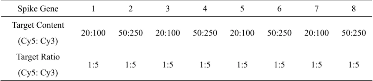
Table 2.3.4-2: Another set of eight spike genes with target contents and ratios in real microarrays. Spike Gene 1 2 3 4 5 6 7 8 Target Content 20 0 50: 0 20: 0 50: 0 20 0 50 0 20 0 50: 0 (Cy5: Cy3) :10 25 10 25 :10 :25 :10 25 Target Ratio (Cy5: Cy3) 1:5 1:5 1:5 1:5 1:5 1:5 1:5 1:5
For those tw sets of microarrays are produced and each
set of microarrays consists of one pair of two dye-swapped microarrays. Therefore,
each type of spike gene is associated with eight microarrays, of which a total of 16
microarrays are tested herein.
The Pearson and concordance correlation coefficient [46] of two random variables
Y1 and Y2 is shown as Eq. (22) and (23):
o types of spike genes, four
, ) , (Y1 Y2 Cov ρ = (22) 2 1 Y Yσ σ 1 2 2 2 1 2 . ( ) ( ( ) ( )) ar Y + E Y −E Y (23) 1 2 ( , ) ( ) c Cov Y Y Var Y V ρ = +
easure the reproducibility among the
ing the log ratios of means
in Cy5 to Cy3 dyes from one microarray image, which is expected to be close to 1. These correlations are used in this study to m
These correlation coefficients of the swapped microarrays are also considered to
evaluate the performance with reference to selected features with high log ratios of
means in Cy5 to Cy3 dyes. As the dyes of Cy3 and Cy5 in the swapped arrays are
exchanged, the negative correlation coefficient is obtained from the features of the
3. Applications on MicroPET Images
This chapter explains the reconstruction and segmentation methods applied to
microPET images. The FBP and OSEM are available methods of the built-in software
of microPET manager V1.6.4 associated with the scanner to reconstruct microPET
image. From our evaluation, the PDEM will demonstrate more accurate and less noisy
reconstruction images than the FBP and OSEM. Moreover, the microPET manager
V1.6.4 does not have any segmentation method for 3D images. Section 3.3 will
present the GMM algorithm to segment 3D microPET images obtained from PDEM.
3.1 The MicroPET Scanner
The microPET R4 scanner in Taipei Veterans General Hospital is shown in Figure
3.1-1. The configuration of this microPET R4 has 32 rings, 6144 detectors, 7.3 cm
field-of-view (FOV), and spatial resolution of 1.85 mm in the center. It can collect
both prompt and delay sinograms. Transaxial projection bin size was 1.213 mm, and
axial slice thickness was 1.2115 mm. Coincidence timing window was set at 6×10⁻⁹
seconds. The lower and upper level energy thresholds were 350 and 750 keV,
respectively. Span of the data set was 3 (Appendix B.5), and maximum ring difference
(MRD) of the data set was 31 (Appendix B.6). The target images were reconstructed
Fig. 3.1-1: The microPET R4 scanner in Taipei Veterans General Hospital is displayed.
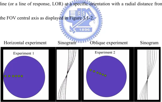
A sinogram uses the polar coordinate system to store the response of a projection
line (or a line of response, LOR) at a specific orientation with a radial distance from
the FOV central axis as displayed in Figure 3.1-2.
Horizontal experiment Sinogram Oblique experiment Sinogram
Fig. 3.1-2: Two images of microPET sinograms from physical experiments of six point sources are displayed. In every sonogram, the horizontal axis represents the ordering of line of responses (LORs) and the vertical axis represents different angles from 0 degree to 180 degree. The pixel intensity in the sinogram records total gamma rays detected in a scanning time window.
During scan acquisition, raw data are stored in sinograms, which are then used to
reconstruct images. The prompt sinogram records coincidence events when two
detectors receive two gamma rays within a specific time window (e.g., 6×10⁻⁹ second).
The coincidence events in prompt sinograms include true, random, and scatter
coincidence events. The delay sinogram records coincidence events when two
detectors receive two gamma rays outside another specific time window (e.g.,
3×6×10-9 second). The coincidence events in delay sinograms can be used to estimate
random coincidence events.
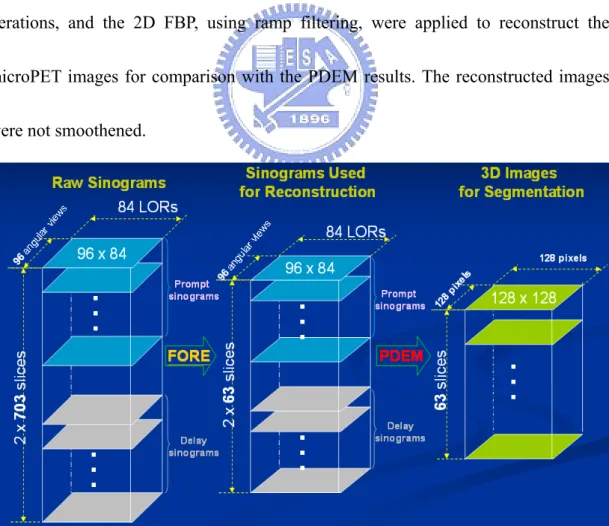
The data matrices are described as follows (as in Fig. 3.1-3 and 3.1-4). First, list
mode data were histogramed into the 3D data with a span of 3 and MRD of 31, which
are sized 2×703×96×84 (that is, 2 sinograms of prompt and delay windows ×703
slices × 96 angular views × 84 projection lines (LORs) as in Fig. 3.1-3) and stored as
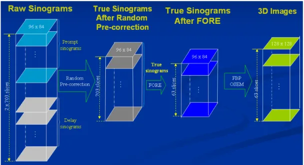
floating type data. The second data were obtained using random pre-correction and
were sized 1×703×96×84 (as in Fig. 3.1-4). These 3D data were rebinned into 2D
sinograms using the FORE method with dead time and decay corrections. The
attenuation, normalization, scattering, and arc corrections were not performed for
simplicity as this study only focused on evaluation of random correction. These
further corrections for PDEM reconstruction will need more investigation in future
Two matrices were constructed using the software embedded in microPET R4 (that
is, microPET manager V1.6.4). The first matrix was 2×63×96×84 (that is, 2 sinograms
of prompt and delay windows × 63 slices × 96 angular views × 84 projection lines
(LORs) as in Fig. 3.1-3) and stored as floating type data. This matrix was
reconstructed using the PDEM. The PDEM was compared with the built-in
reconstruction schemes, such as 2D FBP and OSEM methods, in the microPET R4
system. The second matrix was obtained using the FORE and on-line random
pre-corrected data (as in Fig. 3.1-4). The 2D OSEM, using 16 subsets with four
iterations, and the 2D FBP, using ramp filtering, were applied to reconstruct the
microPET images for comparison with the PDEM results. The reconstructed images
were not smoothened.
Fig. 3.1-3: The above data matrices are used for reconstruction by the PDEM and segmentation by the GMM.
Fig. 3.1-4 The above data matrices are used for reconstruction by the FBP and OSEM with random pre-correction.
3.2 Reconstruction with Random Correction
This section shows the reconstruction results obtained from the PDEM, FBP and
OSEM on simulation, phantoms, and real mouse microPET data.
3.2.1 Simulation Study
This study utilized the modified Shepp-Logan’s head phantom as the simulated
object to assess and compare the reconstruction images using the PDEM, FORE+FBP,
and FORE+OSEM. We assumed that the simulated diameter of a ring was 28.28 mm
and the FOV diameter was 20 mm. Target image was 128×128 pixels (20×20 mm2)
and rescaled intensity was 100. For each pixel intensity, (≤ λt(b)) was simulated and then input into λ*(d)
t . Then, ( )
* d
r
ratio to *(d) t λ . At the end, * p n and * d
n can be simulated using the Poisson
distribution with parameters *(d) t
λ and *(d) r
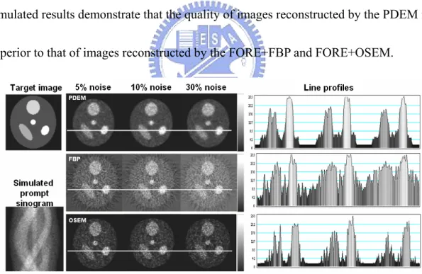
λ as in Eqs. (1) and (2). Total counts (sum of prompt and delayed counts) were 276794, 316383 and 342407 with 5%, 10%
and 30% noise levels, respectively, for the three slices simulated. The prompt and
delayed sinograms had the same matrix size of 96×84 (that is, 96 angular views × 84
projection lines (LORs)) with floating type data. Three random noise ratios of random
to true coincidence counts, 5%, 10% and 30% were simulated. The quality of images
obtained using the PDEM, FBP and OSEM were compared (Fig. 3.2.1-1). The
simulated results demonstrate that the quality of images reconstructed by the PDEM is
superior to that of images reconstructed by the FORE+FBP and FORE+OSEM.
Fig. 3.2.1-1. The modified Shepp-Logan head image was used for simulation studies. The line profiles of PDEM were less noisy than those of FBP and OSEM. The PDEM technique reconstructed better images than the FBP and OSEM did with 5%, 10% and 30% random noise. All images were rescaled using their own maximum values.
3.2.2 Phantom Study
The first physical phantom was 28 homogenous line-sources with an outer diameter
of 1.27 mm for each line. This phantom was utilized to assess the performance and
accuracy of reconstruction quality between the FBP, OSEM and PDEM (as in Fig.
3.2.2-1). The spatial resolution was measured using the FWHMs from vertical and
horizontal line profiles (in Table 3.2.2-1). The average and standard deviation of
FWHMs in reconstruction images using the PDEM were smaller than those obtained
by the FBP and OSEM.
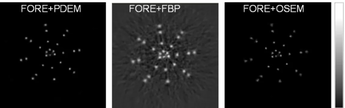
Fig. 3.2.2-1. The 31st slice of the 28 line-source phantom reconstructed using the three methods are displayed. Both FBP and OSEM are reconstruction methods built into the microPET R4 system. All images were rescaled using their own maximum values. The images are shown in the rectangular window. Table 3.2.2-1 presents the comparisons of their FWHMs.
Table 3.2.2-1: Average and standard deviation (in mm) of 28 FWHMs for horizontal and vertical line profiles measured for comparing the spatial resolutions of PDEM, OSEM and FBP. Those values are measured at the 31st slice.
Horizontal profile Vertical profile Methods Average Standard deviation Average Standard deviation
PDEM 1.779 0.324 1.790 0.311
OSEM 1.890 0.527 1.863 0.548
The second phantom was a uniform cylinder of 7.6 cm high with an inner radius of
20 mm. This phantom was also utilized to compare image quality obtained using the
FBP, OSEM and PDEM. Imaging scan time was 1200 s using the microPET R4 after
injection of 276 μCi F-18 FDG. Three reconstruction techniques were applied to
reconstruct the 40th slice (in Fig. 3.2.2-2). Reconstruction images were presented with
the associated central line profiles. Reconstruction images obtaining using the PDEM
had better quality than those generated by the FBP and OSEM on their line profiles. A
circular region of interest (ROI) was employed to measure the noise level for the
different reconstruction methods. The lowest value for coefficient of variation (CV),
which is the ratio of standard deviation to mean, was obtained by using the PDEM
reconstruction (in Table 3.2.2-2).
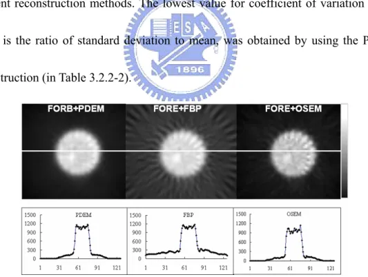
Fig. 3.2.2-2. The reconstructed 40th slice from a uniform phantom was used to investigate noise level generated by the three approaches. The white line indicates the position of the investigated line profile. All images were rescaled using their own maximum values. The images are shown in the rectangular window with enlarged central parts. Table 3.2.2-2 presents the comparisons of their CVs.
Table 3.2.2-2: A circular ROI with a radius of 9 pixels to the center of the uniform phantom was utilized to compare noise levels between the PDEM, FBP and OSEM. Those values were measured at the 40th reconstructed slice.
PDEM FBP OSEM
Average 1146.51 1107.66 1105.36
Standard deviation 36.26 46.82 65.56
Coefficient of variation (%) 3.16 4.23 5.93
The PDEM reconstructed better quality images with lower noise levels than the
reconstructed approaches built into the microPET R4 system during investigations of
line and uniform phantoms. Notably, in all reconstruction processing, there was no
attenuation, scatter, normalization, or arc correction. However, dead time and decay
correction were applied when rebinning 3D sinograms into 2D data.
3.2.3 Real Mouse Study
The PDEM method was applied to real data for small mice to compare the quality
of reconstructed images with those reconstructed using the FBP and OSEM. These
two real normal mice weighed 20 g. Imaging scan time was 600 second using the
microPET R4 following an injection of 0.226 μCi F-18 FDG for the first mouse and
an injection of 240.5 μCi F-18 FDG for the second mouse. The first mouse was
utilized to investigate reconstruction performance under a weak amount of F-18 FDG
activity. The second mouse was used to investigate image quality under a normal
All 63 slices after the FORE were reconstructed using the PDEM, FBP and OSEM.
Figures 3.2.3-1 and 3.2.3-2 present coronal and sagittal images of the two mice
reconstructed by the PDEM. These images are less noisy and have clearer boundaries
than those reconstructed by the FBP and OSEM. These results demonstrate that the
PDEM reconstructed images with better contrast and clearer boundaries than those
reconstructed with the FBP and OSEM.
Fig. 3.2.3-1: Sagittal (top) and coronal (middle) images of the first mouse image reconstructed by PDEM (left), FBP (middle) and OSEM (right). The images reconstructed by PDEM have less noise than those reconstructed using FBP and OSEM with comparison by line profiles. The images are shown in the rectangular window with enlarged central parts.
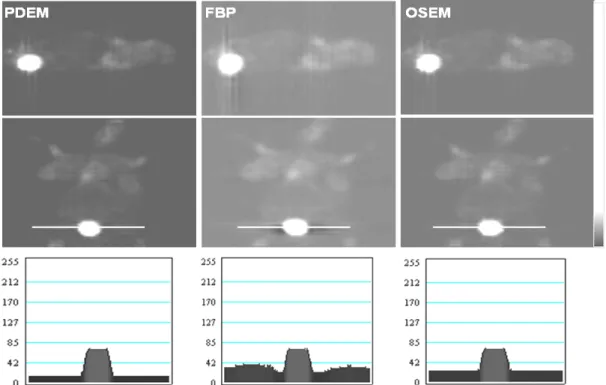
Fig. 3.2.3-2. Coronal and sagittal images of the second mouse image reconstructed using PDEM (left), FBP (middle) and OSEM (right). The images reconstructed by PDEM have less noise than those reconstructed by FBP and OSEM, as shown in the respective line profile near the heart. The images are shown in the rectangular window with enlarged central parts.
3.3 Segmentation of 3D MicroPET Images
This section introduces the use of GMM to segment 3D microPET images from the
reconstruction images by the PDEM.
3.3.1 3D Images
Figure 3.1-3 shows the data matrices used for reconstruction and segemtation.
There are 703 sinograms obtained by the 3D microPET with span 3 and MRD 31. We
applied the FORE on prompt and delay sinograms to obtain 63 sinograms. Each 2D
x 84 and each reconstructed images has the size of 128 x 128. A matrix with the
dimension of 63 x 128 x 128 was used for segmentation by the GMM and K-means
algorithms. The analysis flow chart to segment 3D images is displayed in Fig. 3.3.1-1.
The PDEM is the reconstruction process of microPET images. The GMM or
K-means are applied algorithms for segmentation. The phantoms for simulation
studies are displayed as Fig. 3.3.1-2. There are 63 reconstructed slices with the size of
128 x 128. 2x703 sinograms Obtain 2x63 sinograms by the FORE Reconstruction by the PDEM Smoothing in each slice Segmentation by K-means and GMM 3D segmented images
Slice 1
……. …….
Slice 63
Figure 3.3.1-2: 3D microPET images for 63 slices are illustrated. Every image has the pixels size of 128 by 128.
3.3.2 Simulation Study
The simulated phantom study with 457932 total counts is displayed in Figure
3.3.2-1. This simulated study is focused on testing and evaluating the performance of
GMM. Figure 3.3.2-1A shows target image with five ROIs. Figure 3.3.2-1B displays
target image with 50% noise added. Figure 3.3.2-1C presents the clustering results by
GMM. The number of clusters is decided by the KDE and is shown in Figure
3.3.2-1D. There are four local high peaks that are regarded as the means of four
Fig. 3.3.2-1. A) Simulation image of five clusters is displayed. B) Adding 50% noise into panel A. C) Clustering results using GMM. D) Kernel density curve using C with values of high and low peaks. Four peaks are identified on the density curve. Hence, the number of groups is set as four.
Figure 3.3.2-1 shows the indices of ROIs by the GMM. Figure 3.3.2-3 presents the
accuracy comparison between the simulated results obtained from K-means and
GMM.
Fig. 3.3.2-2. Target ROIs are marked.
Fig. 3.3.2-3. The results of A) by K-means and
B) by GMM clustering are shown.
It is observed that the GMM has a clearer segmentation result than the K-means
method. Results of ROIs are shown in details in Table 3.3.2-1. The total accuracy of
Table 3.3.2-1: Comparisons of the clustering results by K-means and GMM in Fig. 3.3.2-1A.
Exact Counts Accuracy (%) ROI # True Pixel
Count K-means GMM K-means GMM
ROI 1 6604 4128 6206 62.5% 94.0% ROI 2 702 488 522 69.5% 74.4% ROI 3 748 700 745 93.6% 99.6% ROI 4 350 280 285 80.0% 81.4% ROI 5 88 58 59 65.9% 67.0% Total 8492 5654 7817 66.6% 92.1%
Another simulated volume data based on the modified Shepp-Logan's head
phantom image is shown in Figure 3.3.2-4A and 3.3.2-4B. Fifty percentage of noise
ratio to phantom images are added. In order to compare the effects of variation
between slices, different image levels and shapes of ROIs are considered in slice 1
and 2. First, we use the MLEM reconstruction, the result is shown in Figure 3.3.2-4C
and 3.3.2-4D. Meanwhile, the GMM is also applied to segment two images without
slice normalization as shown in Figure 3.3.2-4E and 3.3.2-4F. It is observed that the
boundaries of ROIs are difficult to distinguish. Therefore, slice normalization is
applied to the volume data and then the GMM is used to segment images as shown in
Figure 3.3.2-4G and 3.3.2-4H. The boundaries of these segmentations become clearer
after slice normalization. Figure 3.3.2-4I plots the estimated kernel density curve of
Fig. 3.3.2-4. Simulated volume data including slice 1 and 2 are marked as A and B.
C and D are reconstructed images after added 50% noise ratio to A and B. E and F
are segmented results without slice normalization. G and H are segmented results with slice normalization. I is the estimated kernel density curve of simulated volume data after slice normalization.
For these simulation cases, the performance and accuracy using GMM is better
than those of using K-means. The KDE is adopted to decide the number of clusters
and the starting values of parameters in the EM algorithm. The slice normalization is
necessary when the GMM is applied to segment volume data in this study.
3.3.3 Real Mouse Study
The empirical data of a big mouse injected by F-18 isotope scanning is collected
Scanner energy is between 350 and 750 keV with the total scanning of 3600 s. There
are 32 rings in microPET R4 system. File format of histogram data is stored by 2
bytes for each voxel. Ten slices (from the 51st to the 60th slice) of the volume data are
used for investigation and evaluation.
Figure 3.3.3-1 shows the estimated kernel density curve of volume data. Based on
this KDE, four groups are determined by local high peaks and their starting values are
obtained for applying the EM algorithm.
Fig.3.3.3-1. The estimated kernel density curve using the rat volume data of 10 slices is shown with values of high and low peaks. There are four peaks. Hence, the number of groups is set as four. Values of peaks are applied to compute the starting values in EM algorithm.
Figure 3.3.3-2 shows the reconstructed rat images by MLEM from the 51st to the
60th slice. Besides, Figure 3.3.3-3 and 3.3.3-4 show the segmentation results by GMM
and K-means respectively. The detail segmentation from GMM is shown with the
comparison to Figure 3.3.3-5. The uptake areas can be segmented by GMM from 59th
and 60th images. In addition, it can segment small areas with high gene expression
when compared to K-means. On the contrary, the K-means method segments big areas
For this real mouse study by microPET, the GMM leads to more detail
segmentation results than the K-means method does. The GMM also has better
performance than K-means. The full width half maximum (FWHM) is usually used to
evaluate performance of segmented results. The horizontal line profile near the center
of the 60th slice is used to investigate the performance between GMM and K-means.
Figure 3.3.3-5 is plotted with four regions in this line profile and their FWHMs for
Fig. 3.3.3-2.
Fig. 3.3.3-2. The reconstructed rat images are shown from the 51st (top-left) to the 60th (bottom -right) slice.
Fig. 3.3.3-3. The results of segmentation by the GMM are shown from the 51st (top-left) to the 60th (bottom -right) slice.
Fig. 3.3.3-4. The results of segmentation by the K-means are shown from the 51st (top-left) to the 60th (bottom -right) slice.
Fig. 3.3.3-5. The horizontal line profile of the 60th slice of Fig. 3.3.3-2 is shown with FWHMs. The FWHMs of region 1, 2, 3 and 4 are 3.75, 3.40, 4.14 and 4.45 pixels respectively. The top part shows the location of this line profile in the MLEM reconstruction image and the segmentation by GMM and K-means.
Table 3.3.3-1 shows that the FWHMs of segmented results by GMM are closer to
target FWHMs than those by K-means. Meanwhile, the signal to noise ratio (SNR)
defined by the ratio of mean value to standard deviation is used to compare the
segmentation performance between GMM and K-means. The SNRs of four regions of
GMM are higher than those of K-means.
Table 3.3.3-1: The FWHMs and SNRs of segmented results by GMM are better than those by K-means in Fig. 3.3.3-5.
Pixel of Boundary Signal to Noise Ratio (SNR) Region FWHM of Region GMM K-means GMM K-means 1 3.75 4 7 9.83 6.82 2 3.40 4 6 8.64 6.23 3 4.14 5 7 4.05 2.13 4 4.45 5 7 3.15 2.13
4. Applications on Microarray Images
This chapter investigates the applications of segmentation methods on spotted
microarray images. The GMM and KDE are both employed to segment spotted
images. Furthermore, we combine GMM and KDE to form a new method, GKDE, to
segment spots. The GKDE can keep advantages of KDE and refining the final results
from the GMM. We will compare and evaluate the performance of three methods
together with the adaptive irregular segmentation method in GenePix 6 based on spike
genes, duplicated genes, and swapped arrays in real microarray data.
4.1 The Spotted Microarray Image
These 16 real microarray images used herein are obtained by swapping Cy3 and
Cy5 dyes. Each array has 32 blocks, 15488 spots with 7744 genes. Two replicated
spots are designed in one array, of which the upper 16 blocks are duplicated as the
lower 16 blocks in Fig. 4.1-1. Meanwhile, eight spike genes are designed in each
block to evaluate the performance and accuracy of segmentation methods as shown in
Fig. 4.1-1: An example of microarray image with 32 blocks, 22 columns and 22 rows. One block is enlarged and eight spike genes are numbered.
A typical spot diameter on each microarray in this study is approximately 160 µm.
Sixteen microarray experiments were conducted in Genomic Medicine Research Core
Laboratory of Chang Gung Memorial Hospital, Taiwan. The details of the microarray
experiment procedure and probe information are available on the webpage of the
laboratory,
http://www.cgmh.org.tw/intr/intr2/c32a0/chinese/corelab_intro/genetics/files/03OctCl one_information_F.zip ,
http://www.cgmh.org.tw/intr/intr2/c32a0/chinese/corelab_intro/genetics/files/MIAME %20(GMRCL%20Human%207K)_ver01.zip, and in [42]. These eight pairs of swapped microarrays were used for cancer research. Some of the results have been