適用於可調式小波視訊編碼之訊源機率模型與位元率-失真最佳化方法

(1)

國立交通大學

電子工程學系電子研究所

博士論文

適用於可調式小波視訊編碼之訊源機率模

型與位元率-失真最佳化方法

Source Modeling and Rate-Distortion

Optimization in Scalable Wavelet Video

Coder

研究生：蔡家揚

指導教授：杭學鳴

(2)

適用於可調式小波視訊編碼之訊源機率模型與位元率-失

真最佳化方法

Source Modeling and Rate-Distortion Optimization in

Scalable Wavelet Video Coder

研究生：蔡家揚 Student: Chia-Yang Tsai

指導教授：杭學鳴博士 Advisor: Dr. Hsueh-Ming Hang

國立交通大學

電子工程學系電子研究所

博士論文

A Dissertation

Submitted to Department of Electronics Engineering & Institute of Electronics

College of Electrical and Computer Engineering National Chiao Tung University

in partial Fulfillment of the Requirements for the Degree of

Doctor of Philosophy in

Electronic Engineering October 2010

Hsinchu, Taiwan, Republic of China

(3)

i

適用於可調式小波視訊編碼之訊源機率模型與位元

率-失真最佳化方法

研究生：蔡家揚

指導教授：杭學鳴

國立交通大學電子工程學系電子研究所博士班

摘要

本研究主題可分為兩個主要項目：動態補償(motion-compensated) 差值訊號之訊源模型(source model)以及位元率-失真(rate-distortion)最佳化參數選擇，在第一個項目中，我們發展了零值廣義高斯分佈(ρ-GGD)訊源模型，可準確模擬可調式小波編碼 (scalable wavelet coding)中的訊號機率分佈。我們提出了分段式線性方法可有效率估測在零值廣義高斯模型中的型態參數，並且藉由改善零值機率的估測而提高機率模型之精準度。在第二個項目中，我們提出了一個位元率-失真(rate-distortion)模型用以描述可調式小波視訊編碼中的動態預測效率。可調式編碼架構為開放式迴圈(open-loop)並且同時有多種位元率的編碼需求，與傳統非可調式編碼有很大的不同，也因此傳統上廣泛使用的拉格朗日(Lagrangian)最佳化方法無法良好應用於可調式小波視訊編碼上。為了找到在動態資訊與殘存訊號間最好的位元率分配方法，我們提出了動態資訊增益 (MIG)做為量測動態預測效率指標。基於這項指標，新的代價函式一同被提出。相較於傳統拉格朗日最佳化作法，我們的實驗結果顯示了所提出的模式決定方法可在SNR 與畫面率可調式條件下，擁有較佳的PSNR 表現。

(4)

ii

Source Modeling and Rate-Distortion Optimization in

Scalable Wavelet Video Coder

Student: Chia-Yang Tsai Advisor: Dr. Hsueh-Ming Hang Department of Electronics Engineering & Institute of Electronics

National Chiao Tung University

Abstract

There are two key elements in this study, namely, the source modeling of the motion-compensated prediction error signals, and the coding parameter selection to minimize the rate-distortion criterion. For the first item, we develop an accurate ρ-GGD (Generalized Gaussian Distribution) source model for approximating the signal probability distribution in scalable wavelet coding. An efficient piecewise linear expression is designed to estimate the shape parameter of the ρ-GGD. We also improve the model accuracy in matching the real data by modifying the ρ parameter estimation formula. For the second item, a rate-distortion model for describing the motion prediction efficiency in scalable wavelet video coding is proposed. Different from the conventional non-scalable video coding, the scalable wavelet video coding needs to operate under multiple bitrate conditions and it has an open-loop structure. The conventional Lagrangian multiplier, which is widely used to solve the rate-distortion optimization problems in video coding, does not fit well into the scalable wavelet structure. In order to find the rate-distortion trade-off due to different bits allocated to motion and textual residual information, we suggest a motion information gain (MIG) metric to measure the motion prediction efficiency. Based on this metric, a new cost function for mode decision is proposed. Compared with the conventional Lagrangian optimization, our experimental results show that the new mode decision method

(5)

iii

generally improves the PSNR performance in the combined SNR and temporal scalability cases.

(6)

iv

誌謝

首先要感謝的是我的指導老師杭學鳴教授，在杭老師的指導下，我才能夠逐步學習要如何作研究、要如何培養獨立思考解決問題的能力，在我漫長的研究生生涯中，杭老師總是扮演著貴人的角色。不管是在開會時的討論，論文的修改，或是為人相處上謙沖態度，都讓我學習良多。杭老師尤其提供我許多國際交流的機會，多次參與國際研討會發表，或是兩次在美國 UIUC 交換學生，都讓我在外語能力上有很大的提升，並且感受到不同的學術風氣。另外，還要感謝在 MPEG 合作計畫時，蔣迪豪老師與蔡淳仁老師的指導，讓我有機會可以參與國際標準的寶貴經驗。還要感謝在這一路上陪伴著我的好友們。感謝 CommLab 的老師們、還有許多已畢業未畢業的成員們，讓我可以自在地以實驗室為家，也祝福你們在未來畢業與工作上順利。感謝每星期聚餐的 Wii 組與麻將組大學好友們，讓我星期五的晚上總是充滿美食跟歡樂。還有感謝我的室友們，一同培養各種第二專長，一同度過許多的 AOM 連線及麥當勞外送的夜晚，也祝你們早日博士班畢業。另外還要感謝 PPS 提供的大量美劇，還有 Ptt 的鄉民們，讓我在苦悶的研究生生涯中多了許多樂趣與話題。再來要感謝我的未婚妻珮芬，總是在我研究低潮時給我最有力的鼓勵，總是陪我度過許多的高興與悲傷，一起品嘗美食一同遊玩，答應妳的畢業禮物機車包我會記得送妳的，未來的日子我會努力給你幸福。最後是我親愛的爸媽，沒有你們的支持，我不可能有一絲的成就，你們讓我無後顧之憂安心作研究，並且給我許多寶貴的人生建議，我的學位希望可以榮耀你們，讓你們以我為榮，謝謝你們。家揚 2010.10.17 交大

(7)

v

表目錄

(List of Tables)

Table 3-1. Look-up table for shape parameter estimation ... - 18 -

Table 3-2. K-L divergences of two source models for the 2-D DWT coefficients for image “Lena”. ... - 22 -

Table 3-3. K-L divergence comparison of two source models for temporal-spatial subband coefficients. ... - 22 -

Table 5-1. A 20-SEGMENT SHAPE PARAMETER ESTIMATION TABLE ... - 46 -

Table 6-1. The average frame-level C values using the proposed adaptive scheme ... - 62 -

Table 6-2. The average PSNR results of two different C value scheme ... - 63 -

Table 6-3The default parameter settings [36] of MCTF in Vidwav coder. ... - 83 -

Table 6-4The PSNR Comparison between the Proposed MIG cost method and the Conventional Lagrangian Method in Combined Temporal and SNR Scalability Test for 5 Test Sequences (4CIF Resolution, 60fps) ... - 83 -

(9)

vii

圖目錄

(List of Figures)

Fig. 2-1 The t+2D coding structure of interframe wavelet encoder. The solid line and dashed line show the data paths of the texture and motion information respectively. .... - 7 - Fig. 3-1 An example of wavelet coefficients modeling. (LL-LL-HL subband of image Lena). - 15 - Fig. 3-2 ©(®) at ®∈[0.5, 2.5] and its piecewise linear approximation. ... - 17 - Fig. 3-3 The pdfs of wavelet coefficients (dots) and their approximations by Laplacian

(dotted line) and the proposed ρ-GGD (solid line) models in the subbands: (a) HL, (b) LH, (c) HH, (d) LL-HL, (e) LL-LH, (f) LL-HH. The test image is “Pepper”. ... - 21 - Fig. 4-1 Illustration of rate-distortion curves of texture residual signal before and after

motion prediction. ... - 25 - Fig. 4-2 MSE vs. C value in the MIG cost function at (a) 256Kbps, (b) 284Kbps, and (c)

800Kbps truncation bitrates, and (d) the average MSE for 7 bitrates. (Mobile, CIF resolution). ... - 36 - Fig. 4-3 Flow chart of the proposed mode decision procedure using the MIG cost function- 40 - Fig. 5-1 The solid line and the dashed line are the curves of Ω(α) and its approximating

function Ωe(α), respectively. Ωe(α) is made of 20 line segments in this example.- 43 -

Fig. 5-2 The dots are the probability distribution of the residual absolute-valued signal, xr.

The dashed line and solid line show the approximation results by one-sided Laplacian and ρ-GGD modeling, respectively. The ρ value of the ρ-GGD modeling is estimated based on only the zero probability. Two different cases are shown here: The highest probabilities of the distributions are located at xr=0 (a) and xr=1 (b), respectively. ... - 48 - Fig. 5-3. The solid line and dashed line are the probability distributions of the best a value,

denoted by a*, of the following two cases. The first case is

(solid) and the second case is the opposite (dashed). The five figures show the results at 5 temporal levels: (a) t=0, (b) t=1, (c) t=2, (d) t=3, and (e) t=4. The test sequence is Foreman (CIF, 30fps). ... - 50 - Fig. 5-4. The dotted, dashed and solid lines show the K-L divergence between the

probability distributions ... - 54 - Fig. 5-5. The dotted, dashed and solid lines show the K-L divergence between the

probability distributions ... - 55 - Fig. 6-1. The cost weighting function for α [0.5, 2.5]. ... - 65 - Fig. 6-2. MSE vs. w value with different C0 parameter settings in the MIG cost function: (a)

Mobile (b) Tempete, (c) Container, and (d) Akiyo, all in CIF resolution. ... - 68 - Fig. 6-3. The MSE comparison between the cases with temporal weighting, w=0.8 and w=1,

(10)

viii

Mobile and (b) Foreman. (CIF resolution). ... - 69 - Fig. 6-4. Flow chart of the proposed mode decision procedure ... - 77 - Fig. 6-5. The PSNR comparison between the proposed MIG cost method (solid line) and

the conventional Lagrangian method (dashed line). The test sequences are (a) Container, (b) Irene, (c) Foreman, (d) Tempete, (e) Waterfall, (f) Mobile. (CIF

(11)

- 1 -

Chapter 1 Introduction

Over the past few years, multimedia delivery becomes an important class of wireless/wired internet applications, for example, mobile video and digital TV broadcasting. To overcome the constraints on transmission bandwidth and receiver capability, the scalable coding technique was developed and adopted by the recent international video standards. There are two major approaches on scalable video coding: the DCT-based and the wavelet-based coding schemes. These two coding schemes share many similar coding concepts, especially in removing the temporal redundancy. The Scalable Video Coding (SVC) extension of the H.264/AVC is a representative scheme of the DCT-based approach and has been accepted as the ITU/MPEG standards in 2007 [1]. On the other hand, the wavelet-based coding scheme is a relatively new structure and has its potential and advantages [2] as shown during the MPEG competition process for standardization.

Discrete wavelet transform (DWT) has been successfully applied to still image compression. By exploiting the inter-subband or intra-subband correlation, the DWT transformed image signal can be efficiently compressed by a context-based entropy coder, such as EZW [3], SPIHT [4], and EBCOT [5]. Different from the DCT-based JPEG image coding, the multiresolution property of wavelet transform provides a natural way in producing scalable bitstreams. It enables the spatial and the SNR scalability features in the well-known JPEG2000 image coding standard [6]. In addition to the spatial decomposition,

(12)

- 2 -

DWT can also be applied along the temporal axis and decomposes video frames into temporal subband signals. Therefore, it provides the temporal scalability for videos. In the past fifteen years, the temporal wavelet decomposition is refined by adopting the motion compensated temporal filtering (MCTF) technique. These schemes were proposed and improved by Ohm [7], Hsiang and Woods [8], Secker and Taubman [9], and Xu et al. [10]. MCTF can efficiently decompose video frames along the motion trajectories. After MCTF and spatial 2-D DWT, the original video frames are transformed to spatio-temporal subband signals and compressed by a context-based entropy coder [9], [11]. This interframe wavelet video coding scheme can achieve temporal, spatial and SNR scalability goals simultaneously. Depending on the processing order in the spatio-temporal domain, the scalable wavelet coding methods can be classified to "t+2D" and "2D+t" structures [12]. In this study, we will focus on the t+2D structure.

The rate-distortion analysis of a scalable interframe wavelet video coder is very different from that of a DCT-based coder owing to the following two issues: inter-scale coding and open-loop coding structure. In DCT-based video coders, such as MPEG-2 or H.264, use the hybrid coding technique; all the temporal and spatial prediction operations are basically block-based. Thus, it is quite straightforward to perform the rate-distortion analysis along the coding operation flow. On the other hand, in the interframe wavelet coders, the temporal MCTF is performed block-wise, but the spatial entropy coding is performed on the

(13)

- 3 -

subbands. This inconsistent data partition increases the rate-distortion analysis difficulty drastically. Wang and Schaar proposed a solution in [13] to analyze the rate-distortion behavior across different coding scales for wavelet video coder. The second issue is that the DCT-based video coder has a closed-loop coding structure. The prediction errors within the loop can be controlled by adjusting coding parameters [14]; thus, the optimal rate-constrained motion compensation can be adaptively adjusted [15],[16]. But the interframe wavelet coding has an open-loop prediction structure and the quantization process is performed after all the encoding operations are completed. This open-loop scheme provides more flexibility on bitstream extraction and robustness to transmission errors, but it has no feedback path to provide useful information to adjust prediction parameters in the encoding process. Therefore, it is difficult to achieve the rate-distortion optimization target, especially in the case of allocating bits between the motion and the texture data at multiple operation points all at the same time. How to generate adequate amount of motion information and decide the best prediction modes for MCTF becomes a challenging problem in the scalable interframe wavelet video coding.

Our objective is to develop a rate-distortion optimization method to improve the coding performance of scalable wavelet video coding. For building an efficient rate-distortion model, we propose an accurate source model. Moreover, we also suggest a piecewise linear method to estimate the shape parameter of the Model. Besides, we derive an analytical

(14)

- 4 -

model that describes the trade-off between the motion compensation bits and the residual texture coefficients bits. We then allocate bits to each category properly at different scalability dimensions. We first examine the rate-distortion effect due to the increase or decrease of motion information bits. Then we derive a quantitative expression to measure the motion prediction efficiency. Most significantly, we give a theoretical explanation to this metric from the entropy viewpoint. Based on this finding, a new cost function is proposed. By minimizing the proposed cost function, the best prediction mode is decided and the corresponding motion vectors are chosen for the MCTF operation. Compared with the mode decision procedure in the conventional scalable wavelet video coder, the proposed method shows a PSNR improvement for the combined SNR and temporal scalability cases. The proposed methods are also published in [38] and [39].

This thesis is organized as follows. Chapter 2 gives a brief review of interframe wavelet video and the rate-distortion mechanisms in video coding. In Chapter 3, the ρ-GGD source modeling is proposed to approximate the probability distribution of wavelet coefficients. In Chapter 4, we suggest the motion information gain (MIG) metric to measure the motion prediction efficiency. According to our source model, the MIG metric is further discussed from the entropy viewpoint. Extending the work in Chapter 3, the ρ-GGD source model is improved by an enhanced estimation method of the ρ value. The one-sided ρ-GGD is proposed for the texture residual signal in Chapter 5. In Chapter 6, the two concepts, MIG

(15)

- 5 -

in Chapter 4 and one-sided ρ-GGD in Chapter 5, are integrated into a complete and working algorithm. The major contributions in this thesis are listed as follows.

Contributions of this Study

(1) An accurate and efficient source model, ρ-GGD, is proposed to approximate the probability distribution of the wavelet coefficients.

(2) A quantitative metric, MIG, is proposed to measure the motion prediction efficiency of MCTF.

(3) Based on the MIG metric, a new rate-distortion cost function is proposed for mode decision. The parameters of the MIG cost function are empirically selected.

(4) To further improve the ρ-GGD model, the one-sided ρ-GGD model and an more reliable estimation method on ρ are proposed to approximate the probability distribution of residual texture signal.

(5) Based on MIG and one-sided ρ-GGD, an integrated MIG mode decision algorithm is developed. The parameters of the cost function are first theoretically derived and then fine-tuned by experimental data.

(16)

- 6 -

Chapter 2 Scalable Wavelet Video

Coding and Its Rate-Distortion

Optimization

2.1 Brief Introduction to Interframe Wavelet

Video Coding

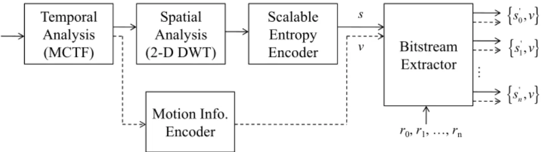
The most popular coding structure of interframe wavelet video codec is the so-called “t+2D” structure as shown in Fig. 2-1. The order of “t+2D” implies the encoding operation order: the temporal analysis first and then the spatial analysis. The temporal analysis employs the MCTF technique. It decomposes a group of pictures (GOP) into several temporal high-pass frames and one low-pass frame along the motion vector trajectories. The motion information portion is, in the conventional approach, nonscalable, which is denoted as v in Fig. 2-1. Then, the spatial decomposition operation (2-D DWT) is applied to the low-pass and high-pass frames to form subbands for further quantization and entropy coding. With the help of a scalable entropy coder, these spatio-temporal subbands are compressed to a scalable bitstream, denoted as s in Fig. 2-1. Therefore, the coded output bitstream consists of two parts, one is the scalable bitstream for the texture information (s) and the other is the non-scalable bitstream for the motion information (v); together, they are denoted as {s, v}. To fulfill the application requirements imposed on the video bitrates, image resolution, and frame rate, the texture bitstream is truncated accordingly but the motion bitstream remains intact. Therefore, the output bitstreams of the bitstream extractor are {s0’, v}, {s1’, v}… {sn’, v} to match the scalable requirements r0, r0,…, rn, respectively,

(17)

- 7 -

entropy coder.

The EBCOT [5] image coding algorithm is adopted by the JPEG2000 standard, and similar algorithms are widely adopted by the state-of-art wavelet video codecs [9], [11]. The basic coding flow of an interframe wavelet video coder is as follows. After temporal and spatial analysis, each subband is partitioned into a number of code blocks, and the bitplanes of each block are processed by a few coding paths. The boundary between two consecutive coding paths is a truncation point. These truncation points are characterized by the slopes of the rate-distortion curves at the truncation point. These slope values are recorded and sent to the bitstream extractor. In one extraction unit, such as one GOP, the coding paths with similar slopes are grouped into the same coding layer. A permissible positive slope value is called a rate-distortion threshold. The coding layers with the absolute values of their slopes higher than the rate-distortion threshold are chosen to form an output bitstream. The sum of the bitrates of these chosen coding layers is calculated. If the calculated bitrate is less than the target bitrate, the rate-distortion threshold is adjusted to a smaller value so that more coding layers will be included and the total bitrate increases. On the other hand, the threshold value increases so as to discard some coding layers. By repeating the above operation, the bitrate of the truncated bitstream reaches the target value. Because each bitplane of a code block is split into three coding paths, the bitrate extraction can be quite

Fig. 2-1 The t+2D coding structure of interframe wavelet encoder. The solid line and dashed line show the data paths of the texture and motion information respectively.

Temporal Analysis (MCTF) Spatial Analysis (2-D DWT) Scalable Entropy Encoder Motion Info. Encoder Bitstream Extractor r₀, r₁, …, r_n s v

{ }

' 0, s v

{ }

' 1, s v

{ }

'_, n s v …

(18)

- 8 -

accurate. Therefore, the bitrate of the texture bitstream can be precisely controlled by the bitstream truncation mechanism. But the non-scalable motion information imposes a constraint on bitstream scalability. The motion information is typically temporal scalable and can be adapted to different decoding frame rates. However, when the spatial scalability feature is turned on, the motion information is often not adjustable to different decoding picture size during the extraction. In the following sub-section, we will compare the rate-distortion optimization methods for the non-scalable and the scalable video cases, and then develop the methods in the next section to adjust the motion information bitrate.

(19)

- 9 -

2.2 Rate-Distortion Mechanism in Video Coding

According to the Shannon’s source coding theory [18], the rate-distortion function can be derived from the probability model of a coding source. Based on the rate-distortion function and with the help of optimization methods, an optimal rate-distortion trade-off can be theoretically obtained for a given bitrate or distortion condition.

In a typical hybrid video coding scheme, the coding source is the transformed residual signal after inter or intra predictions. It is well known that the probability distribution of the transformed coefficients can be closely approximated by the Laplacian distribution [21]

, (1) where Λ is the Laplacian parameter and can be estimated from the signal standard deviation by . If the probability distribution of the transformed residual signal is a Laplacian source, its rate-distortion function with quantization distortion D and texture coding rate R was derived in [18]. In addition to the texture coding bit rate, the extra side information needed in a hybrid coder is mostly the motion information rate ΔR. According to the optimization theory, the best motion prediction mode can be obtained by minimizing the Lagrangian cost function defined by

, (2) where λMode is the Lagrange parameter. For a fixed ΔR, can be theoretically derived for a well-defined rate-distortion function in (2). Both the theory and the real data show that

(20)

- 10 -

the value is strongly related to the quantization step size, which controls the amount of distortion directly [22], [23]. Different values are used by several popular reference encoders. These values are picked or derived based on their system characteristics and the experimental data [24]. The rate-constrained motion estimation is performed separately by using another Lagrangian cost function given by

, (3) where FD is a function of the frame difference between the original and the reconstructed image blocks. In many practical systems, FD is either SSD (sum of squared differences) or SAD (sum of absolute differences). In the MPEG reference encoder, is empirically chosen to be and for SSD and SAD, respectively [22].

From (2) and(3), is, clearly, an important factor that balances the weights of rate and distortion in the overall cost (J) and it thus affects the bitrates allocated to the texture and the motion information. As discussed earlier, depends on the source characteristics, the quantization step size and the bit rate. Several papers [19], [20] show that the statistics of the texture are helpful in selecting the proper value. The key for solving the mode decision and bit allocation problem is to find the relationship between quantization step size, texture characteristics and bit rate.

Using only one fully self-embedded bitstream to satisfy different coding requirements simultaneously is the most attractive feature of the scalable video coding technique. In the

(21)

- 11 -

scalable interframe wavelet coding, the bitstream generation process and bitstream extraction process are two separate, independent steps. The encoding process generates lossless compressed bitstream. After the encoding, the extractor truncates the lossless bitstream according to the bitrate requirement. In other words, the extractor plays the role of quantizer. This coding structure uses the input source frames, not the reconstructed frames, to predict the current frame. It is often referred as “open-loop structure” in the 3D wavelet coding literature [12]. It is very difficult to precisely control the prediction accuracy during the encoding process. Moreover, multiple bitstreams are to be extracted from the same coded bitstream. It is hard to adequately allocate the motion information bitrates at encoder (before the extractor) to satisfy all target operation points simultaneously. A theoretical treatment on the optimum trade-off between the motion information bitrate and the texture signal bitrate for a motion-compensated video codec was earlier explored by Girod [15] and will be discussed in the next section. In practice, most existing scalable wavelet video coding schemes still adopt the cost functions used in the hybrid video coding ((2) and (3)), but the Lagrange parameter in each temporal decomposition stage is manually selected empirically [25]. Because the target bitrate is given after the entire bitstream is coded, the pre-selected, fixed-value Lagrange parameter must be working for a range of bitrates. In other words, we hope it can provide a reasonable overall performance for all the bitrates of interest. The cost function defined by (2) determines the best motion prediction mode. If a

(22)

- 12 -

total bitrate is given, we can follow the conventional approach to pick up the Lagrange parameter. But unfortunately, the bitrate is not known at the encoding stage for scalable wavelet video encoding.

To go one step further, we look into the role that the motion vectors play in scalable interframe wavelet coding. The MCTF unit performs the temporal decomposition operation along the motion trajectory; therefore, the accuracy of motion vectors is critical to their motion compensation performance. The low-pass frames produced by temporal filtering will be further decomposed at the next temporal level. Thus, the temporal decomposition layers form a hierarchical structure. The inefficiency in motion prediction propagates along the temporal hierarchy in the same GOP. Therefore, accurate motion vectors tend to decrease the overall distortion. But, a very accurate motion vector often requires more coding bits.

To sum up, the Lagrangian cost function is a very powerful tool in the conventional non-scalable coder. But due to the open-loop coding structure and the requirement of multiple operating points, the use of the Lagrangian cost function in scalable wavelet video coding becomes inadequate. The key problem is finding the proper trade-off between the motion information and the residual texture information for scalable wavelet video coder. The whole scenario becomes even more complicated when we consider the propagation of MCTF inefficiency along temporal hierarchy. Therefore, we propose another approach to

(23)

- 13 -

(24)

- 14 -

Chapter 3 ρ-GGD Source Modeling

for Wavelet Coefficients

2-D Image signal can be decomposed twice by a 1-D discrete wavelet transform (DWT) into a 2-D multi-resolution representation. Each 1-D DWT splits the 2-D image signal into low-pass (L) and high-pass (H) subbands along the vertical or the horizontal direction. Typically, the LL subband is further split several times in image coding. In an interframe wavelet video coding structure, another wavelet filter bank is applied along the motion trajectory of moving objects [7]. The temporal L frame is often a moving average of frames, while the temporal H frame contains the frame differences. In video coding, these temporal L and H frames are further decomposed by the spatial 2-D DWT, so all original frames in a GOP are transformed to a temporal-spatial subband representation.

For either image or video coding, the source modeling is critical in the R-D analysis. The pdf (probability density function) of wavelet coefficients has been modeled as a generalized Gaussian distribution (GGD) [26][27]. To construct a GGD source model, the pdf variance and kurtosis have to be calculated first in order to estimate the shape parameter.

(25)

- 15 -

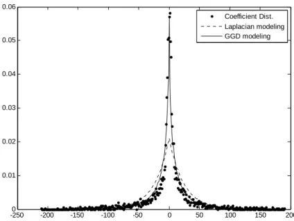
Variance and kurtosis are related to the second and the forth moments. Therefore, the process of constructing a GGD model is rather complicated. To reduce the complexity, the Laplacian distribution is often adopted. Although the Laplacian source model is thus widely used, its coefficients approximation errors are sometimes high as shown in Fig. 3-1. Therefore, we propose a ρ-GGD source model in the next section to achieve the high accuracy of the GGD model but with lower complexity.

Fig. 3-1 An example of wavelet coefficients modeling. (LL-LL-HL subband of image Lena).

-2500 -200 -150 -100 -50 0 50 100 150 200 0.01 0.02 0.03 0.04 0.05 0.06 Coefficient Dist. Laplacian modeling GGD modeling

(26)

- 16 -

3.1 ρ-GGD Source Model Derivation

The pdf of wavelet coefficients typically has zero-mean. Thus, the generalized Gaussian distribution (GGD) source model is given by

, (4)

where

, (5) Here, σ is the standard deviation of wavelet coefficients, v is the shape parameter of the GGD model, and Γ(x) is the standard Gamma function. Let ρ be the probability of

zero-value coefficients. According to(4), ρ is given by

, (6)

Therefore, (4) can be rewritten by the following ρ-GGD representation:

, (7)

In building a ρ-GGD source model, the shape parameter v has to be estimated first. From (5) and (6), the product of ρ and σ can be written as

, (8) (8) shows a mapping relationship between the shape parameter v and the product of ρ and σ in the ρ-GGD model; that is, ½¾ = ©(®). Because parameters ρ and σ can easily be obtained from data, it is convenient to use their product to estimate the value of ©(®).

(27)

- 17 -

From experiments, the range of ® is [0.5, 2.5] for typical image/video wavelet coefficients. In Fig. 3-2 , the solid line shows the values of Φ(®) in the range of ®_∈[0.5, 2.5], an decreasing one-to-one function of ®. Therefore, the inverse function of Φ(®) at ®_∈ [0.5, 2.5] exists and is unique; thus, the shape parameter ® can be estimated from Φ-1(ρσ).

Fig. 3-2 ©(®) at ®∈[0.5, 2.5] and its piecewise linear approximation.

0.5 1 1.5 2 2.5 0 0.5 1 1.5 2 2.5 3 v Φ(v) Φ_est(v)

(28)

- 18 -

3.2 Piecewise Linear Estimation for the Shape

Parameter of Wavelet Coefficients

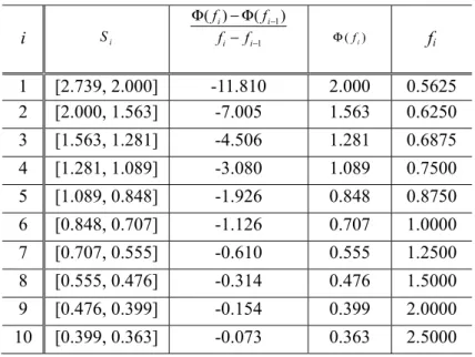
In Fig. 3-2, ©(®) is an exponentially decreasing smooth curve. We found experimentally that ©(®) can be approximated accurately for ®∈[0.5, 2.5] by piecewise linear approximation. We partition the ©(®) curve into ten pieces for ®∈[0.5, 2.5]. For each piece at ® 2 [fi; fi¡1], ©est(®) is approximated by a linear model as below

, (9)

where i={1,2,…10} and {f0, f1, f2, f3, f4, f5, f6, f7, f8, f9, f10}= {0.5, 0.5625, 0.625, 0.6875, 0.75,

0.875, 1, 1.25, 1.5, 2, 2.5}. Fig. 3-2 shows that ©(®) is well approximated by ©est(®). And the shape parameter can be estimated by , which is

, (10)

Table 3-1. Look-up table for shape parameter estimation

i Si 1 1) ( ) ( − − − Φ − Φ i i i i f f f f ) (fi Φ fi 1 [2.739, 2.000] -11.810 2.000 0.5625 2 [2.000, 1.563] -7.005 1.563 0.6250 3 [1.563, 1.281] -4.506 1.281 0.6875 4 [1.281, 1.089] -3.080 1.089 0.7500 5 [1.089, 0.848] -1.926 0.848 0.8750 6 [0.848, 0.707] -1.126 0.707 1.0000 7 [0.707, 0.555] -0.610 0.555 1.2500 8 [0.555, 0.476] -0.314 0.476 1.5000 9 [0.476, 0.399] -0.154 0.399 2.0000 10 [0.399, 0.363] -0.073 0.363 2.5000

(29)

- 19 -

when

, (11)

Furthermore, a look-up table of the constants used in (10) and (11) can be pre-calculated as shown in Table 3-1. In conclusion, a ρ-GGD model for the pdfs of wavelet coefficients can be constructed by using the following steps:

Step 1: Compute ρ and σ from the wavelet coefficients.

Step 2: Use Table 3-1 to get Si in (11) based on the product of ρ and σ and also the corresponding model coefficients.

Step 3: Calculate the estimated shape parameter ®est from (10) using the model coefficients obtained in Step 2.

(30)

- 20 -

3.3 Modeling Accuracy Evaluation

The difference between two probability distributions can be evaluated by estimating the relative entropy or the said Kullback- Leibler (K-L) divergence [28]. In this thesis, we use the symmetric definition defined by

, (12)

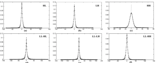
where p is the “true” pdf and q is the “modeling” pdf. A small K-L divergence means a higher modeling accuracy. The experimental results of the ρ-GGD and the Laplacian modeling are compared for several test cases. In the spatial 2-D DWT case, the Daubechies 9/7 biorthogonal wavelet filter [29] popular in image coding is adopted in our experiments. Fig. 3-3 shows the pdfs of the spatial subband coefficients and their models for the test image “Pepper”. It is clear that the ρ-GGD model matches the real pdf much better than the Laplacian model in all spatial subbands. Table 3-2 shows the divergence of our model and the real pdf by using the symmetric K-L divergence for the test image “Lena”. In general, the ρ-GGD model outperforms the Laplacian significantly in all subbands except for the LH subband.

(31)

- 21 -

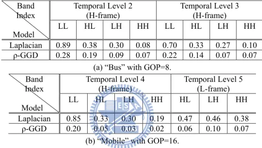
In the interframe wavelet video case [10], the temporal-spatial subband coefficients are produced by using MCTF and the spatial 2-D DWT. Table 3-3 shows the results of the K-L divergence estimation of two test sequences, “Bus” and “Mobile”, with GOP=8 and 16 respectively at CIF resolution. The ρ-GGD model shows a much better modeling accuracy than the Laplacian. In general, the higher subband signals are difficult to model but the ρ-GGD model shows good accuracy in Table 3-3 (b) even at deep temporal subbands.

From the experimental results, the ρ-GGD model shows a very good modeling performance in both spatial 2-D DWT and interframe wavelet video cases. Compared to the Laplacian model, the ρ-GGD has a much better accuracy and consistency in modeling the pdfs of wavelet coefficients.

Fig. 3-3 The pdfs of wavelet coefficients (dots) and their approximations by Laplacian (dotted line) and the proposed ρ-GGD (solid line) models in the subbands: (a) HL, (b) LH, (c) HH, (d)

LL-HL, (e) LL-LH, (f) LL-HH. The test image is “Pepper”.

HL LH HH LL-HL LL-LH LL-HH (a) (b) (c) (d) (e) (f) HL LH HH LL-HL LL-LH LL-HH (a) (b) (c) (d) (e) (f)

(32)

- 22 -

Table 3-2. K-L divergences of two source models for the 2-D DWT coefficients for image “Lena”. Band Index Model HL LH HH LL- HL LL- LH LL- HH Laplacian 0.22 0.07 0.03 0.68 0.52 0.42 ρ-GGD 0.16 0.08 0.03 0.22 0.21 0.20

Table 3-3. K-L divergence comparison of two source models for temporal-spatial subband coefficients. Band Index Model Temporal Level 2 (H-frame) Temporal Level 3 (H-frame) LL HL LH HH LL HL LH HH Laplacian 0.89 0.38 0.30 0.08 0.70 0.33 0.27 0.10 ρ-GGD 0.28 0.19 0.09 0.07 0.22 0.14 0.07 0.07 (a) “Bus” with GOP=8.

Band Index Model Temporal Level 4 (H-frame) Temporal Level 5 (L-frame) LL HL LH HH HL LH HH Laplacian 0.85 0.33 0.30 0.19 0.47 0.46 0.38 ρ-GGD 0.20 0.05 0.03 0.02 0.06 0.10 0.07

(33)

- 23 -

Chapter 4 Motion Information Gain

(MIG) and Mode Decision Method

A typical extraction process in scalable wavelet coding truncates only the encoded texture bitstream and maintains the integrity of the entire encoded motion information. For a given bitrate condition, different amounts of motion information lead to different types of residual texture signals, and thus lead to different rate-distortion behavior. Although there are other approximate solutions [29], [31] that select the scalable motion information to match certain very low-bitrate requirements, we focus on the pre-partitioned motion information solution in the following study. That is, the optimal amount of information bits is decided at the encoding stage. We first analyze the rate-distortion behavior of the motion-predicted residual signals. Then, based on this rate-distortion relationship, we derive a quantitative metric that measures the coding efficiency of motion information. Also, a theoretical explanation from the entropy viewpoint is given to our coding efficiency metric.

(34)

- 24 -

4.1 Rate-Distortion Model of

Motion-Compensated Prediction

For a scalable wavelet video coder, theoretically, we can fix an extraction bitrate and then find the rate-distortion behavior due to the increase/decrease of motion information. In other words, at a given bit rate, if a certain amount of the texture bit rate is shifted to the motion information, will the reconstructed image distortion be reduced or increased? A solution to this problem is searching for the optimal motion information that leads to the optimal R-D performance at different bit rates. For example, is the block size or the motion vector accuracy more important in improving the coded image quality? Clearly, the answer depends on both picture content and bit-rate.

Although the residual frames after MCTF will be further spatially decomposed by 2-D DWT, in this study we focus on the rate-distortion behavior of the texture information at the MCTF stage (not after 2-D DWT) because the motion information coding efficiency is our main concern. Because the consecutive frames are often very similar, the motion-predicted residual signals typically have zero-mean and nearly symmetrical distribution. The residual signals after motion prediction can be modeled as Laplacian sources. Because the temporal high-pass frame is essentially a weighted combination of the motion-predicted residual frames, we next try to construct the rate-distortion model of the motion-compensated residual signals.

(35)

- 25 -

When the residual texture signal is produced by the motion prediction operation, the rate-distortion behavior of this texture information portion is decided. That is, since the residuals are fixed after motion compensation, their rate and distortion trade-off due to quantization and entropy coding is also fixed. However, if we change the motion vectors (mv) used in motion prediction, the residual signals are different and thus, the texture rate-distortion function changes. We like to know the texture rate-distortion function variation before and after the motion prediction being applied to the same coding block.

For a motion-compensated video codec, Girod [15] pointed out that at a given total bit rate, the optimum trade-off point should locate at

, (13)

where the left hand side is the distortion decrease due to texture rate increase and the right

Fig. 4-1 Illustration of rate-distortion curves of texture residual signal before and after motion prediction. T R T R − ΔR R D 0( T) D R ( _T ) D R_v _{− Δ}R 0( ) D R ( ) D R_v

(36)

- 26 -

hand is the distortion decrease due to motion information rate increase. Fig. 4-1 gives an illustration of this principle. We use the zero motion vector (no motion-compensation) case as a reference. In Fig. 4-1, D0 (R) is the rate-distortion function of the residual signal

produced by using the zero motion vector, and Dv (R) is the rate-distortion function of the

residual signals produced with the motion vector set v. From the bitrate viewpoint, an extra coding bitrate ΔRis needed for sending the motion vectors v. Since the total target bitrate RT is given, the bitrate available for the texture information is reduced to RT -ΔR. If this set of mv is beneficial for the overall performance, the quantization error (distortion) of the texture information with mv should be less than that without mv at the same target bitrate. Otherwise, the motion compensation is judged inefficient. Therefore, the distortion with motion prediction is smaller than that without motion prediction:

. (14) Conceptually, (14) is equivalent to (13) in [15]. But different from the motion region partition approach in [15], we try to find an instrumental trade-off measure and a design procedure for adjusting the mv bit rate.

For the Laplacian source described by (1), if the absolute-error distortion measurement is in use, (14) can be rewritten using the rate-distortion functions given in [18] as

. (15) The Laplacian parameter and can be estimated from the residual signal variances,

(37)

- 27 -

and , respectively. That is, . Thus, (15) becomes

. (16) Let us define the function Φ to be the logarithm value of the signal standard deviation, and let ΔΦ be

. (17) Then, (16) can be rewritten as

. (18) From (14) to (18), we can see that the target bitrate term RT is cancelled because it appears on both sides in (15). This target bitrate elimination gives us a big advantage in the rest of our rate-distortion analysis. Different from the conventional video coding, the target (extraction) bitrate is unknown during the scalable encoding process. In this formulation, the measurement of motion prediction efficiency is extraction bitrate irrelevant. This is true under the assumption that the residual signal probability distribution is Laplacian for both with and without motion-compensated prediction. This Laplacian model is not all accurate in real cases. Here, ΔΦ and ΔR represent the variation of texture statistics and the bitrate cost of adopting motion estimation, respectively. We thus view ΔΦ/ΔR as a gain factor in measuring the motion prediction efficiency. Intuitively, the motion prediction operation is preferred if it reduces the texture variance significantly. Furthermore, (18) gives a quantitative metric and specifies a threshold of acceptable ΔΦ/ΔR. This threshold is derived

(38)

- 28 -

(39)

- 29 -

4.2 Motion Information Gain (MIG)

According to the last sub-section, ΔΦ represents the variation of texture statistics due to motion-compensated prediction. We are going to show next that ΔΦ represents the difference between two differential entropies. For the Laplacian source X, its differential entropy h(X) is given below [18].

, (19)

where Λ is the Laplacian parameter. Thus, the differential entropies of the residual signals and produced by the zero motion vector and the motion vector set v are, respectively,

. (20)

Although the differential entropy does not represent the actual bitrate, the difference between two differential entropies represents the bitrate difference estimation of these two sources. Since the Laplacian parameter can be estimated from the signal variance, we thus obtain the following equation:

. (21) Comparing (21) with (17), as a consequence of rate-distortion theory on the Laplacian source, we find that these two equations are the same. Therefore, ΔΦ represents the reduction of residual signal entropy in encoding the residual signals before and after motion-compensated prediction. Thus, the interpretation of ΔΦ/ΔR is as follows.

(40)

- 30 -

From (22), we can see that ΔΦ/ΔR is the ratio of the “reward” and the “cost” due to the use of motion-compensated prediction. The “cost” is the extra bitrate for encoding the motion vectors, and the “reward” is the entropy reduction of the residual texture signals. Therefore, ΔΦ/ΔRis called the “motion information gain”, abbreviated as MIG. It is thus used to measure the motion prediction efficiency. We denote this MIG function due to the motion vector set v by

. (23) This gain factor implicitly represents the trade-off between the residual signal bitrate and motion information bitrate. The fundamental concept behind (23) is similar to that (13) in [15] as discussed earlier. But through our preceding lengthy derivation, we show that the total target bitrate disappears in the final MIG expression. Thus, the MIG metric fits well for applying to the scalable wavelet video coding structure.

Let us extend the original criterion (18) to a more general form. When we consider the advantage of using motion- prediction in scalable wavelet video coding, the MIG metric of the candidate motion vector set v should satisfy

, (24) where C is a chosen threshold value. In the original derivation, C is 1. Here we investigate the range of C values in real video coding cases. Because a practical entropy coder cannot approach the entropy bound, both the compressed texture and the compressed motion information would need more bits to code. Therefore, the motion prediction is not as effective as (14) shows. The distortion reduction by the motion bitrate , measured in bits/pixel, is less than the expected value; that is, should be larger in real cases. Therefore, (14) is modified to

(41)

- 31 -

where . Using the above equation, we can follow the same derivation process in section III.A to obtain the MIG lower bound. Consequently, an inequality similar (16) is derived:

. (26) Because , the right term of the above equation, the lower bound of C, is larger than 1. When is small or is large, C becomes much larger than 1.

(42)

- 32 -

4.3 MIG Cost Function

Since our motion mode and vector selection process is applied only to image blocks with non-zero optimal motion vectors, the denominator of (23) is non-zero. There are a few interesting properties associated with .

1) _{. Clearly, we will not use an mv that produces a negative ΔΦ value. For a} given image block, if the zero mv is the best mv in the sense that any non-zero mv cannot reduce the residual signal variance, then the value associated with this block is assigned to be 0 and the best coding mode is the one with the zero motion vector.

2) is bounded. In digital image coding, the residual signal has a finite variance. The best non-zero mv can, at the best, reduce the residual variance to zero. The variance difference before and after employing mv is thus finite. In other words, the value saturates and cannot be further improved when a proper mv is identified.

3) In the following sections, we deal mainly with the case that . That is, the useful mv, v, should produce a value greater than 0 and less than or equal to . Ideally, the parameter C is 1 and is independent of image contents and target bit rate if the Laplacian rate-distortion model holds. However, as discussed earlier, practically C is not 1 and is bitrate dependent.

Intuitively, the MIG metric with the constraint, , can be the cost function used for searching for the optimal mv. However, the C value is unknown and to be

(43)

- 33 -

identified in real image coding. Thus, for the convenience in computation, we use the following equivalent form. We expand (24) with the aid of (17) and (23). The inequality becomes

. (27) A large MIG value implies a large ΔΦ and/or a small ΔR. In (17), a large ΔΦ value implies that the difference between and is large. Thus, the right term in (27), , should be as small as possible. Therefore, we propose a so-called “MIG cost function” to measure the prediction cost. For a coding source s, the motion vector set v produces the residual signals with variance _{and its average information bitrate (for representing v)} is ΔR(v). The MIG cost function J is defined as

, (28) where C is generally source and bit-rate dependent. We include it explicitly in the argument of the J function to emphasize its role in our rate control algorithm. The problem now becomes looking for v that minimizes J.

We need to identify the value of C in (28). According to our previous discussions, the C value is decided by the coding system and the source signal s in (23). In practice, the source signal s is the temporal high-pass frames generated by MCTF. Indeed, the probability distributions of the different temporal layers have different shapes [32]. We conduct the following experiments to characterize J and also to identify the value of C.

(44)

- 34 -

We start with a fixed C value and simply use (28) as the cost function in performing motion estimation and mode decision in encoding. The detailed procedure of mode decision will be described in the next sub-section. After the encoding process is done, the encoded bitstream is truncated to a fixed bitrate, for example, 256kbps, and then we decode the truncated bitstream. The mean-squared error (MSE) between the decoded and the original images is calculated; thus, one test point of a MSE and C pair is obtained. The data are collected from 32 frames of the Mobile sequence at CIF resolution.

Repeating the above steps with different C values, we obtain a MSE vs. C curve at 256Kbps as shown in Fig. 4-2 (a). By changing the truncation bitrates settings, the MSE vs.

C curves at 384Kbps and 800Kbps are obtained as shown in Fig. 4-2 (c) and (d) respectively.

Each ofFig. 4-2 (a)(b)(c) shows that the MSE is minimal when C reaches a certain value. This is equivalent to the performance saturation phenomenon we discuss earlier. When C is large, only the very effective mv’s can make positive contribution and their value is diminishing as C gets larger; and thus the MSE goes up again as shown in Fig. 4-2 (a)(b)(c). Although the theory predicts that MIG is independent of bit rate, in reality, however, the coding system efficiency and the source probability distribution are bitrate and temporal level dependent. Indeed, the best C value that leads to the minimum MSE tends to be smaller at higher bitrates. This is consistent with the known observation that the mathematical model matches the real rate-distortion relationship at higher rates. For

(45)

- 35 -

example, the rate-distortion relationship of a quantizer approximates the asymptotical R-D function at high bitrates [18]. If the optimum C value does not change significantly, we prefer to use a constant C to cover the bitrates of our interests. We pick up seven target bitrates, 256k, 384k, 512k, 800k, 1024k, 1200k, and 1500k, and their average behavior (MSE vs. C) is shown in Fig. 4-2 (d). In conclusion, the C value generally falls in the range of [4, 10].

(46)

- 36 -

(a) (b)

(c) (d)

Fig. 4-2 MSE vs. C value in the MIG cost function at (a) 256Kbps, (b) 284Kbps, and (c) 800Kbps truncation bitrates, and (d) the average MSE for 7 bitrates. (Mobile, CIF resolution).

100 102 104 106 108 110 112 114 116 3 4 5 6 7 8 9 10 11 12 13 14 MSE C 256kbps 69 69.5 70 70.5 71 71.5 72 72.5 73 3 4 5 6 7 8 9 10 11 12 MS E C 384kbps 34.5 34.7 34.9 35.1 35.3 35.5 35.7 35.9 36.1 36.3 36.5 2 3 4 5 6 7 8 9 10 11 12 13 MSE C 800kbps 46.5 47 47.5 48 48.5 49 49.5 3 4 5 6 7 8 9 10 11 12 MSE C

(47)

- 37 -

4.4 Block-Based Mode Decision Procedure

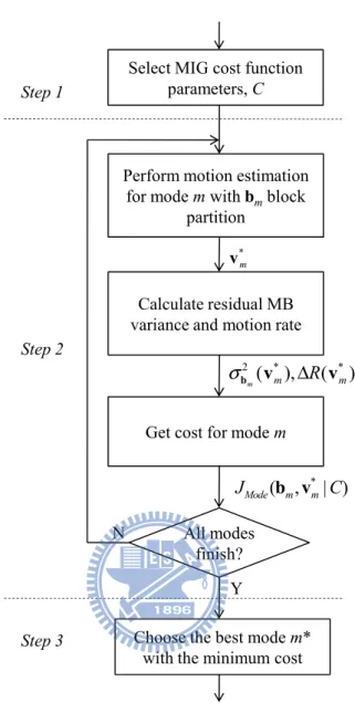
The MIG cost function can be used to decide the coding mode. It tells us the trade-off between the motion information and the texture information. Based on MIG, we develop a mode decision procedure. In a conventional non-scalable video coder, the best motion vector and coding mode are decided by minimizing the Lagrangian cost function ((2) and (3)) for a given single bitrate. As discussed in the previous sub-sections, with the MIG cost function we are able to choose the most appropriate coding mode (including mv) by minimizing its value. The basic steps in the proposed mode decision procedure are similar to that in the conventional scheme. In the existing scalable wavelet video coding schemes, the mv search is block-based and the variable block-size motion compensation technique is used to find the best macroblock coding mode. Each macroblock coding mode represents a partition of macroblock into a certain combination of sub-blocks. Fig. 4-3 illustrates the proposed mode decision procedure, which consists of three steps as described below.

1) Step 1: Select the appropriate MIG cost function parameters

The proposed MIG cost function contains one parameter, C. According to our previous discussions, C can be empirically chosen from the intervals, [4, 10]

2) Step2: Search for the best motion vector set for each block mode

There are many possible sub-block combinations for motion compensation in one macroblock. For example, a typical 16x16 size macroblock has 16x16, 16x8, 8x16, and

(48)

- 38 -

8x8 block modes; and each 8x8 block can be further partitioned to 8x4, 4x8, and 4x4 sub-blocks. Assuming that a macroblock can be partitioned to Nm sub-blocks for mode m, the mv’s (vi) associated with all sub-blocks (bi) form two Nm-tuple vectors, vm and bm, respectively, where

. (29) For each sub-block, to find the best mv, all the mv candidates within the search range S are examined. These candidate motion vectors can have forward, backward or bi-directional prediction directions. By minimizing the MIG cost function in (28), the best motion vector for sub-block bi is obtained. Mathematically, it is identified by performing the following optimization procedure.

. (30)

Then, the best mv for the macroblock is the collection of all the best motion vectors for mode m; i.e.,

. (31) The residual signal is modeled as a Laplacian source with zero-mean. After all the sub-blocks finish the motion estimation process for mode m, the residual variance and the average motion information bitrate of a macroblock can be, respectively, expressed as

(49)

- 39 -

, (32)

where rm is the average extra bits needed to record the coding mode information. Both and are in bits/pixel.

3) Step 3: Choose the best block mode with the minimum MIG cost

Assuming that the block mode m in Step 2 belongs to the mode set M, which contains all possible block modes, the MIG cost function in (28) is used again to choose the best macroblock mode. Hence, the best block mode is decided by minimizing the MIG cost function:

. (33)

(50)

- 40 -

Fig. 4-3 Flow chart of the proposed mode decision procedure using the MIG cost function

Select MIG cost function parameters, C

Perform motion estimation for mode m with b_mblock

partition

Calculate residual MB variance and motion rate

* m v 2 ₍ *_), ₍ *₎ m m R m σb v Δ v

Get cost for mode m

All modes finish? * ( , | ) Mode m m J b v C Y N

Choose the best mode m* with the minimum cost

Step 1

Step 2

(51)

- 41 -

Chapter 5 One-Sided ρ-GGD Source

Modeling for Residual Signals

In the study of motion estimation efficiency, an accurate source model on the motion-compensated residual signal is critical and essential. The results in [32] show that the ρ-GGD source model is more accurate than the Laplacian model. Because we use, typically, a non-negative metric on the prediction errors such as MAD or SSD (Sum of Squared Difference), we propose the so-call one-sided ρ-GGD model to approximate the probability distribution of the absolute-valued residual signals. In the modeling process, we propose an efficient linear method to estimate the shape parameter. Furthermore, we increase the modeling accuracy on the real data by proposing an improved ρ value selection method.

(52)

- 42 -

5.1 One-Sided ρ-GGD Function

The probability distribution of the motion-compensated residual signal can be approximated by a zero mean and symmetric probability density function (pdf), and the GGD model is a good example [27]. The GGD pdf is given by

, (34)

where

, (35)

and α is the shape parameter; Γ(·) and exp(·) are the Gamma function and the exponential function, respectively. The σ parameter represents the standard deviation of the residual signal. We now like to approximate the probability distribution of the absolute values of the residual signals. Let the source sample be denoted as x_∈X , where X is the source

alphabet set. Because (34) is a zero-mean and symmetric pdf and X is non-negative, we modify the GGD model to the one-sided GGD with the following pdf:

. (36)

The shape parameter α in (36) can be estimated by using the variance and kurtosis of the source signal [27] but the complexity of this approach is very high. We will derive an

(53)

- 43 -

alternative expression that can be computed from the data samples with much less computation.

We denote the probability of zero in (36) by ρ. That is,

. (37)

And then (36) can be rewritten as

. (38)

We name (38) the one-sided ρ-GGD. There is an interesting property of the proposed one-sided ρ-GGD. From (35) and (37), the product of ρ2 and σ2 can be rewritten as

. (39)

That is, the product of the square of zero-value probability and the variance is a function of

α. We denote this function as

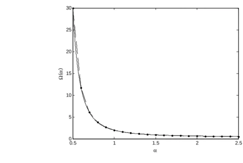
Fig. 5-1 The solid line and the dashed line are the curves of Ω(α) and its approximating function Ωe(α), respectively. Ωe(α) is made of 20 line segments in this example.

0.5 1 1.5 2 2.5 0 5 10 15 20 25 30 α Ω (α )

(54)

- 44 -

. (40) This functional relationship is useful in estimating the shape parameter. As Fig. 5-1 shows, the mapping between Ω(α) and α is one-to-one. Therefore, the inverse function of Ω(α) exists. According to (39) and (40), α can be obtained by

. (41) Different from the conventional approach, we develop a new and fast method to estimate the shape parameter based on the expression of (41). That is, we use the zero-value probability and the variance value to estimate α.

(55)

- 45 -

5.2 Piecewise Linear Estimation of Shape

Parameter of Residual Signal

Fig. 5-1 shows that Ω(α) is an exponentially decreasing function of the argument α. Ω(α) can be divided into a number of segments and each segment is approximated by a straight line. The entire range of α is [α0, αn]. We uniformly partition it into n segments. Thus, Ω(α) curve is approximated

by n pieces of line segments; these line segments are specified by the n sets of boundary points: {Ω(α0), Ω(α1)}, {Ω(α1), Ω(α2)} …,and {Ω(αn-1), Ω(αn)}. That is, Ω(α) is approximated by a

piecewise linear function Ωe(α). For the i-th segment,

, (42)

where α∈[αi-1, αi]. Generally, the approximation is more accurate for large n. Fig. 5-1 shows the

example of n=20, and Ω(α) is rather accurately approximated by Ωe(α) in this case.

The linear function defined by (42) clearly has an inverse. We can thus estimate the shape parameter αe using (41). If both ρ and σ2 are known, then

(56)

- 46 -

for

. (44) One may notice that the coefficients in (43) are independent of data and can thus be calculated in advance and recorded on a table. Table 5-1 shows the example of n=20. Therefore, for the i-th line segment, the coefficients can be retrieved from Table I, and then the shape parameter can be estimated by using (43).

Table 5-1. A 20-SEGMENT SHAPE PARAMETER ESTIMATION TABLE

i Ω(αi−1) Ω( )αi 1 1 ( ) ( ) ( ) i i i i i i α α α _{α α} − α − Ω −Ω Ω − − 1 1 ( )i ( i ) i i α α α α− − Ω −Ω − 1 30 11.7 121.3 -182.6 2 11.7 6.12 45.49 -56.25 3 6.12 3.8 22.34 -23.18 4 3.8 2.65 13.01 -11.51 5 2.65 2 8.5 -6.5 6 2 1.6 6.023 -4.023 7 1.6 1.33 4.532 -2.667 8 1.33 1.14 3.568 -1.865 9 1.14 1.01 2.911 -1.359 10 1.01 0.91 2.442 -1.024 11 0.91 0.83 2.096 -0.793 12 0.83 0.76 1.833 -0.629 13 0.76 0.71 1.628 -0.508 14 0.71 0.67 1.464 -0.417 15 0.67 0.64 1.332 -0.348 16 0.64 0.61 1.223 -0.293 17 0.61 0.58 1.132 -0.25 18 0.58 0.56 1.056 -0.215 19 0.56 0.54 0.99 -0.187 20 0.54 0.53 0.934 -0.163

(57)

- 47 -

5.3 Improved ρ Estimation

In the above discussion, ρ is defined as the zero-value probability of the one-sided ρ-GGD. In the one-sided ρ-GGD model, ρ also represents the highest probability value of the model. However, for some residual image macroblocks, zero is not the most probable value. In this case, using the zero probability to estimate ρ does not lead to good approximation. Therefore, we modify the ρ estimation formula for this special case.

Fig. 5-2 shows two cases. To plot the probability derived from data, the residual absolute-valued signal is rounded to its nearest integer and is denoted by xr; the probability distribution of xr and its modeling results are shown in Fig. 5-2. In the case of Fig. 5-2 (a), the zero probability, , is the highest probability, and thus the one-sided ρ-GGD can well approximates the data distribution. However, in the case of Fig. 5-2 (b), because is not the peak probability and it results in poor approximation. Therefore, we propose a modified estimation formula for ρ. Although the mean of the real residual signal may not be zero, it is not far away from zero based on our collected data. We thus use both the probability of zero, , and the probability of one, , to estimate ρ: that is, ρ is the linear combination of two probabilities,

(58)

- 48 -

(45)

(a)

(b)

Fig. 5-2 The dots are the probability distribution of the residual absolute-valued signal, xr. The dashed

line and solid line show the approximation results by one-sided Laplacian and ρ-GGD modeling, respectively. The ρ value of the ρ-GGD modeling is estimated based on only the zero probability. Two different cases are shown here: The highest probabilities of the distributions are located at xr=0 (a) and

xr=1 (b), respectively. 0 2 4 6 8 10 12 14 16 18 0 0.1 0.2 0.3 0.4 0.5 0.6 0.7

Rounded residual absolute value x

r P ro b a b ilit y 0 2 4 6 8 10 12 14 16 18 0 0.05 0.1 0.15 0.2 0.25 0.3 0.35 0.4 0.45 0.5

Rounded residual absolute value x

r

P

robabi

lit

(59)

- 49 -

and . In order to find the optimal a value, we test the following a values, {0, 0.1, 0.2, 0.3, 0.4, 0.5, 0.6, 0.7, 0.8, 0.9, 1}, and examine the one-sided ρ-GGD modeling results for each a value. The a value that leads to the most accurate approximation is chosen to calculate the ρ value. To evaluate the modeling accuracy, we use the K-L (Kullback-Leibler) divergence as (12). Therefore, for each residual macroblock, we can choose the best a value, denoted by a*,

, (46) where P is the probability distribution of the residual absolute-valued signal; is defined by (38) and its ρ value is estimated using (45). Although (17) can be used in the off-line analysis, it is impractical in processing real data. We thus develop an efficient method for determining the a* value.

We separate all events into two cases: and the opposite. At each temporal level, we collect the a* values of all macroblocks, and separate them into two bins according to the preceding two cases. The probability distributions of a* of these two cases are shown in Fig. 5-3. In the case of , the most probable a* value is 1 and its probability is over 90%. Therefore, when the first case occurs, a* is chosen to be 1. Otherwise, 0 is chosen to be the value of a*. In other words,

(60)

- 50 -

In summary, the probability distribution of the residual absolute-valued signal can be

(a) (b)

(c) (d)

(e)

Fig. 5-3. The solid line and dashed line are the probability distributions of the best a value, denoted by a*, of the following two cases. The first case is (solid) and the second case is the opposite (dashed). The five figures show the results at 5 temporal levels: (a) t=0, (b) t=1, (c) t=2, (d) t=3,

and (e) t=4. The test sequence is Foreman (CIF, 30fps). 0 0.1 0.2 0.3 0.4 0.5 0.6 0.7 0.8 0.9 1 0 0.1 0.2 0.3 0.4 0.5 0.6 0.7 0.8 0.9 a* P robabi lit y 0 0.1 0.2 0.3 0.4 0.5 0.6 0.7 0.8 0.9 1 0 0.1 0.2 0.3 0.4 0.5 0.6 0.7 0.8 0.9 1 a* P robabi lit y 0 0.1 0.2 0.3 0.4 0.5 0.6 0.7 0.8 0.9 1 0 0.1 0.2 0.3 0.4 0.5 0.6 0.7 0.8 0.9 1 a* P robabi lit y 0 0.1 0.2 0.3 0.4 0.5 0.6 0.7 0.8 0.9 1 0 0.1 0.2 0.3 0.4 0.5 0.6 0.7 0.8 0.9 1 a* P roba bi lit y 0 0.1 0.2 0.3 0.4 0.5 0.6 0.7 0.8 0.9 1 0 0.1 0.2 0.3 0.4 0.5 0.6 0.7 0.8 0.9 1 a* P rob abi lit y

(61)

- 51 -

approximated by the proposed one-sided ρ-GGD source model by the following steps.

Step 1: Calculate the variance σ2 from the motion-compensated residual signals.

Step 2: Estimate the ρ value using (45) and (47).

Step 3: Compute the product of ρ2 and σ2.

Step 4: Using TABLE I, we can find the interval [Ω(αi-1), Ω(αi)] that the ρ2σ2 value belongs to.

Step 5: Pick up the i-th segment coefficients from TABLE I. The shape parameter αe is

estimated by using (43).

適用於可調式小波視訊編碼之訊源機率模型與位元率-失真最佳化方法

國 立 交 通 大 學

電子工程學系 電子研究所

博 士 論 文

適用於可調式小波視訊編碼之訊源機率模

型與位元率-失真最佳化方法

Source Modeling and Rate-Distortion

Optimization in Scalable Wavelet Video

Coder

研 究 生： 蔡 家 揚

指導教授： 杭 學 鳴

適用於可調式小波視訊編碼之訊源機率模型與位元率-失

真最佳化方法

Source Modeling and Rate-Distortion Optimization in

Scalable Wavelet Video Coder

研 究 生：蔡 家 揚 Student: Chia-Yang Tsai

指導教授：杭 學 鳴 博士 Advisor: Dr. Hsueh-Ming Hang

國 立 交 通 大 學

電子工程學系 電子研究所

博 士 論 文

適用於可調式小波視訊編碼之訊源機率模型與位元

率-失真最佳化方法

研究生：蔡家揚

指導教授：杭學鳴

國立交通大學 電子工程學系 電子研究所博士班

摘要

Source Modeling and Rate-Distortion Optimization in

Scalable Wavelet Video Coder

Abstract

誌謝

目錄

表目錄

(List of Tables)

圖目錄

(List of Figures)

Chapter 1 Introduction

Chapter 2 Scalable Wavelet Video

Coding and Its Rate-Distortion

Optimization

2.1 Brief Introduction to Interframe Wavelet

Video Coding

{ }

{ }

{ }

2.2 Rate-Distortion Mechanism in Video Coding

Chapter 3 ρ-GGD Source Modeling

for Wavelet Coefficients

3.1 ρ-GGD Source Model Derivation

3.2 Piecewise Linear Estimation for the Shape

Parameter of Wavelet Coefficients

3.3 Modeling Accuracy Evaluation

Chapter 4 Motion Information Gain

(MIG) and Mode Decision Method

4.1 Rate-Distortion Model of

Motion-Compensated Prediction

4.2 Motion Information Gain (MIG)

4.3 MIG Cost Function

4.4 Block-Based Mode Decision Procedure

Chapter 5 One-Sided ρ-GGD Source

Modeling for Residual Signals

5.1 One-Sided ρ-GGD Function

5.2 Piecewise Linear Estimation of Shape

Parameter of Residual Signal

5.3 Improved ρ Estimation

國立交通大學

電子工程學系電子研究所

博士論文

研究生：蔡家揚

指導教授：杭學鳴

研究生：蔡家揚 Student: Chia-Yang Tsai

指導教授：杭學鳴博士 Advisor: Dr. Hsueh-Ming Hang

國立交通大學

電子工程學系電子研究所

博士論文

國立交通大學電子工程學系電子研究所博士班