預測使用者行為以輔助身份辨識的融合統計方法

國 立 交 通 大 學

網路工程研究所

碩 士 論 文

預測使用者行為以輔助身份辨識的融合統計

方法

Predicting User Behavior for Identity Verification by Fusion

of Statistical Methods

研 究 生：劉仁倩

指導教授：謝續平 教授

預測使用者行為以輔助身份辨識的融合統計方法

Predicting User Behavior for Identity Verification by

Fusion of Statistical Methods

研 究 生：劉仁倩 Student：Jen-Chien Liu

指導教授：謝續平 博士 Advisor：Dr. Shiuhpyng Shieh

國 立 交 通 大 學

網 路 工 程 研 究 所

碩 士 論 文

A Thesis

Submitted to Institute of Network Engineering

College of Computer Science

National Chiao Tung University

in partial Fulfillment of the Requirements

for the Degree of

Master

in

Computer Science

June 2007

Hsinchu, Taiwan, Republic of China

預測使用者行為以輔助身份辨識的融合統計方法

研究生：劉仁倩 指導教授：謝續平

國立交通大學 網路工程研究所

摘 要

已有許多研究提出利用生物特徵辨識技術來輔助傳統帳號密碼方式的身份 認證。然而，不管是哪種生物特徵，往往都會隨著時間而有所改變，特別是行為 特徵。因此，在本論文中，除了使用者敲鍵行為本身的特徵外，亦將敲鍵行為的 改變趨勢視為使用者的另一項特徵，藉此預測使用者目前最可能的行為。本篇論 文提出結合高斯模型、自動回歸預測模型，及統計學習理論中的隱藏馬可夫模型， 以建立敲鍵行為特徵預測的統計機率模型，利用此機率模型分析使用者登入帳號 密碼的時間資訊是否符合該身份擁有的特徵，藉此降低身份冒用的風險。實驗結 果顯示，本論文所提出的方法可使錯誤辨識率降至 2.19%，相較於過去其他相關研 究（通常高於 3%），甚至我們之前的研究成果（2.54%）都來得更準確。特別是當 使用者敲鍵行為資料具有特定變動趨勢時，藉由行為預測可使辨識準確率有效提 升。

Predicting User Behavior for Identity Verification by

Fusion of Statistical Methods

Student: Jen-Chien Liu Advisor: Shiuhpyng Shieh

Department of Computer Science

National Chiao Tung University

Abstract

Biometric verification mechanism has been used to complement the traditional password-based authentication system. However, the biometrics may change over time, especially for behavioral biometrics. In this thesis, the keystroke typing characteristics are not the only features used, but also the tendency of change in keystroke behavior. The most likelihood behavior of user will be predicted to verify the user. In this paper, we propose a fusion model for predictive keystroke analysis inspired by Gaussian Model, Autoregressive Model, and Hidden Markov Model. This model predicts the keying behavior of a user based on his past statistical information. Results of the experiment showed that, the EER could down to 2.19%, which is better than other works in literature to our knowledge (generally higher than 3%), and even better than our previous work (2.54%). Especially as users type with some trend or regularly, their identified accuracy could be enhanced by predicting their keying behavior.

誌

謝

首先感謝指導教授謝續平教授兩年來的諄諄教誨，尤其讓我出國參加 ACM conference 發表論文，一方面感謝老師對我的看重，一方面也感謝老師給予我機會 能有這樣難得的經驗。另外，感謝實驗室的學長姐們，在我研究的過程中給予許 多寶貴的意見，特別感謝子逸學長在我論文遇到瓶頸的時候，幫我指引方向，讓 我能順利完成。感謝一起奮鬥的碩二同學們，你們一直給予我信心鼓勵，讓我在 最艱難的時候能夠繼續撐下去。感謝碩一的學弟妹們，多虧了你們的幫忙，讓我 們能專心準備論文口試。感謝所有對於本研究提供實驗資料的朋友們，讓我的實 驗能夠順利完成。 最後要感謝我的家人，提供我所需，並讓我無後顧之憂的專注於研究。感謝 小 A 先生，謝謝你這段時間對我的包容與支持，也謝謝你陪伴我度過各式各樣的 難關。祝福所有人，事事順心如意！

This work was supported in part by Taiwan Information Security Center (TWISC), National Science Council under the grants NSC 95-2218-E-001-001, and NSC95-2218-E-011-015.

Table of Contents

1. INTRODUCTION... 1

2. RELATED WORK... 5

2.1 Methods of Keystroke Analysis ... 5

2.2 Behavior Change... 7

2.3 Summary ... 8

3. PROPOSED MODEL... 10

3.1 Definitions... 10

3.2 Modeling n-graph by Gaussian Model... 11

3.3 Estimating Probable Parameters by Autoregressive (AR) Model... 13

3.4 Hidden Markov Model for Sequential Keystroke Analysis ... 16

3.5 Authentication Scheme ... 19

4. EXPERIMENTS AND RESULTS... 26

4.1 Experiment Settings ... 26 4.2 Data Collection ... 27 4.3 Ideal Cases ... 27 4.4 Results ... 29 4.5 Discussion ... 31 5. CONCLUSION... 34 6. REFERENCES... 35

List of Figures

FIGURE 3.1: THE DISTRIBUTION OF DIGRAPH DURATION... 12

FIGURE 3.2: THE HIDDEN MARKOV MODE... 16

FIGURE 3.3: THE HMMS FOR KEYSTROKE ANALYSIS... 17

FIGURE 3.4: HIDDEN MARKOV MODEL FOR KEYSTROKE SEQUENCE “PAPAYA” ... 18

FIGURE 3.5: THE GRAPHICAL MODEL FOR DIGRAPHS WITH SEQUENCE “PAPAYA” ... 18

FIGURE 3.6: FLOW CHART OF THE TRAINING PHASE FOR FIXED-TEXT KEYSTROKE ANALYSIS ... 20

FIGURE 3.7: THE PROCEDURES OF PROFILE BUILDING MODULE... 21

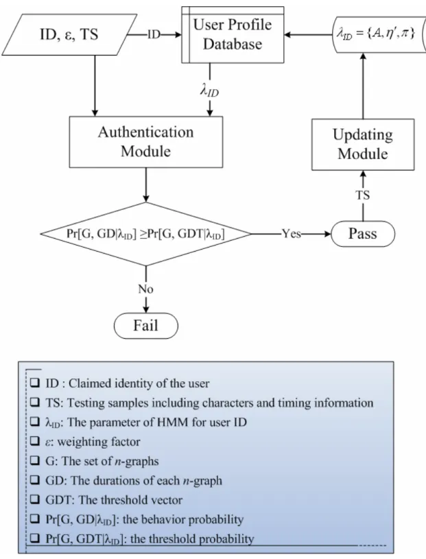
FIGURE 3.8: FLOW CHART OF RECOGNITION PHASE AND RETRAINING PHASE... 23

FIGURE 3.9: THE PROCEDURES OF AUTHENTICATION MODULE... 24

FIGURE 3.10: THE PROCEDURES OF UPDATING MODULE... 25

FIGURE 4.1: THE DISTRIBUTION OF NUMBER OF SAMPLE DATA... 27

FIGURE 4.2: THE FOUR CASES WITH DIFFERENT BEHAVIOR CHANGE... 29

FIGURE 4.3: EQUAL ERROR RATE (EER) OR AVERAGE FALSE RATE (AFR) FOR SEVERAL APPROACHES ( GREEN BAR: APPLY MACHINE LEARNING METHODS; BLUE BAR: APPLY STATISTICAL CLASSIFICATION METHODS)... 32

List of Tables

TABLE 4.1: THE EER COMPARATIVE RESULTS OF PREDICTIVE AND NON-PREDICTIVE MODEL

... 28

TABLE 4.2: ANALYSIS RESULTS OF FOUR CASES WITH DIFFERENT BEHAVIOR CHANGE... 29

TABLE 4.3: COMPARATIVE RESULTS OF EER IN EXPERIMENT... 30

TABLE 4.4: THE RATIOS OF USERS HAVING IMPROVED EER ... 30

TABLE 4.5: THE AVERAGE PROMOTION OF EER WITH DIFFERENT ORDER OF AR MODEL IN THE EXPERIMENT... 31

TABLE 4.6: THE MAXIMUM PROMOTION OF EER WITH DIFFERENT ORDER OF AR MODEL IN THE EXPERIMENT... 31

1. Introduction

With the rapid evolution of computer and internet technology, more and more users take the privacy of themselves seriously. User’s private information is often delivered through the internet for some web-based services or network applications, such as E-commerce, webmail, web storage, and Blog, etc. Before gaining access to these services or applications, authentication is needed to verify the user’s identity. The conventional authentication system usually employs the username-password pair to verify user’s identity, which only checks the correctness of character combinations. However, the password-based authentication system has the vulnerability of suffering form malicious attacks and intrusion. If the adversary steals the victim’s username-password pair, he can gain access to the services by masquerading as the victim. To deal with this problem, a biometric verification mechanism is needed to complement traditional authentication.

Biometric technologies measure and analyze human physiological or behavioral characteristics. Physiological biometrics requires a user provide some physical characteristic, such as fingerprint, facial recognition, hand geometry, iris scan, retinal scan, vascular patterns, and DNA. Unfortunately, most involve expensive hardware to support the dedicated function. As a result, additional cost is required to combine with the authentication mechanism. Behavioral biometrics, which includes keystroke dynamics, speech recognition, hand-writing, and mouse movement, usually requires a user to behave in a consistent manner.

Nevertheless, the biometrics may change over time, especially for behavioral biometric. Taking the typing behavior as the example, when a user chooses an unfamiliar string as the username or password, or the user is strange to type, he must type the string slowly and erratically. After a while, the user may become familiar to

type the string. Since he need not stop and think what character is next, the typing speed will be much faster. Even for physiological biometrics, the physiological characteristics still could change over a long time. For example, as the user gets older, his face will be different than before.

There are rarely works mentioning about this factor. If the authentication system did not consider this, the probability of false rejecting legal user will raise over time. The authentication system will become unusable. On the other side, if the user’s behavior can be predictable according to previous behavior, the abnormal behavior of imposter should be detected easily. The probability of legal user passing the authentication will be not affected or even better.

Keystroke dynamics, also referred to as keyboard typing characteristics or keyboard typing rhythms, is one of the behavioral biometric that has several key advantages over other biometric technologies:

- It is non-intrusive since the user already utilizes the keyboard for input.

- It is transparent because keystroke patterns can be captured silently without interrupting the user’s normal activity.

- It is low-cost since the keyboard is the only hardware needed, and the analysis can be implemented in software.

Although different keyboard may affect a user’s typing characteristics and the environment may influence the user’s behavior, keystroke dynamics is considered to be an economical and practical technique to enhance conventional authentication methods. We will apply the sequential data prediction method to keystroke behavior for identity verification.

Keystroke dynamics is based on the assumption that different people have unique habitual rhythm patterns in the way they type. It is seen as a good evidence of identity [7][18]. Depending upon the structures of the typing pattern, keystroke dynamics falls

into two categories: fixed-text keystroke analysis and free-text keystroke analysis. In the fixed-text keystroke analysis, the patterns are short, fixed and structured, such as username-password pair at the authentication phase. The methods [3][8][14][20][22] proposed for fixed-text keystroke analysis typically integrate with or replace the traditional web-based authentication method. In contrast, the free-text keystroke analysis patterns are diverse and long; they can be collections of keys a user types in a period of time. Free-text keystroke analysis [7][15][24] is suitable for continuous identity verification after the authentication phase.

The typing behavior is not always suitable for identifying user. If the user’s typing behavior is irregular and wayward, the user’s typing behavior is hard to distinguish. In our work, we assume that the users need to login or provide typing sample to the authentication system frequently, such as webmail, daily work applications, etc. And the user’s typing behavior change with some tendency, so the typing behavior can be predicted.

In this thesis, we present a formal statistical model for keystroke dynamics analysis using Gaussian Modeling, Autoregressive Model, and Hidden Markov Model. The keystroke sequence will first be divided as several parts. Each part will be model by Gaussian model and Autoregressive model. The Gaussian Model is used to calculate the possibility that some behavior belongs to some user, and the parameters of Gaussian Modeling are estimated by Autoregressive Model. Then, we apply the Hidden Markov Model to model the user’s sequential keystroke behavior. Based on proposed model, we develop scheme for fixed-text keystroke analysis, which can be applied to web-based services to enhance the security strength of conventional authentication mechanisms. Our proposed model can be also extended to free-text keystroke analysis for identification. Experimental results indicated that the EER could down to 2.19%. It is better than other works in literature to our knowledge (generally higher than 3%), and

even better than our previous work (2.54%) [27]. Especially as users type with some trend or regularly, their identified accuracy could be enhanced by predicting their keying behavior.

The remainder of this thesis is organized as follows. We discuss the related works of keystroke dynamics in Chapter 2, and propose a formal model along with the scheme for fixed-text keystroke analysis in Chapter 3. Chapter 4 presents our experimental results and discussions, while Chapter 5 gives the conclusion and direction for future work.

2. Related Work

There have been many works using the keystroke dynamics to verify the user’s identity. The features of keystroke dynamics include timing features (duration, hold time, latency, and so on), pressure, and position. Most works analyzed user’s keystroke by using the timing features. This idea was first appeared in 1975 [1]. Later, a number of researchers have begun to propose various analysis methods for keystroke dynamics, and a commercial product suite ware shown up [40]. In this chapter, the keystroke analysis methods which are proposed in related works will be first introduced in Section 2.1. Then Section 2.2 focuses on the behavior change and Section 2.3 gives a summary of related works.

2.1 Methods of Keystroke Analysis

The analysis methods of most works can be classified as two categories: statistical classification methods and machine learning methods. The former includes simple statistical methods and data mining methods, such as k-nearest neighbor decision rule, Bayes classifier, and decision tree. The latter includes Neural Network, Fuzzy Logic, Support Vector Machine, and Hidden Markov Model, etc.

2.1.1 Statistical Classification Method

Early works applied the statistical classification method form statistics or data mining area to analyze the typist’s keystroke characteristics. Gaines et al [2] made an experiment which 7 professional secretaries were asked typing some predetermined text, and used t-test method to examine the typing characteristics. Joyce and Gupta [3] introduced an intuitive method to analyze the user’s login name, first name, last name,

and password during the login process. They measured the difference between the reference strings and the test strings, and compared the difference with some threshold. Monrose and Rubin [7] [13] clustered users based on the typing speed with three classifier methods: Euclidean distance measure, non-weighted probability, and weighted probability measure. Their work focused on analyzing the most frequent appeared digraph. Magalhaes et al [22] introduced a lightweight algorithm to analyze keystroke characteristics and considered the concept of keyboard gridding based on Revett and Khan’s work [23]. Guven et al [38] introduced a vector based algorithm which is similar to minimum distance classifier. They calculated norms of the vector dimensions for a given two keystroke vectors to make a decision. Hocquet et al [21] combined three classification methods – classical method (the average and standard deviation), measurement of the disorder, and using a discretization of the time. Villani et al [24] analyzed the long-text input to verify user’s identity with the nearest neighbor classifier. They made experiments using two input modes – copy and free-text input, and two keyboard types – desktop and laptop keyboards.

In these works, the typing string length is usually longer than 14 for accuracy, but the error rate is still higher than 5%.

2.1.2 Machine Learning Method

Recently, most works utilize the machine learning methods to model the user’s typing behavior, and the verification accuracy is improved. The Neural Network [5][6][10] was applied in this area from 1997. Then Ru et al [8] and Araújo et al [20] utilized the Fuzzy Logic to distinguish users based on the keystroke latencies, the distance of the keys on the keyboard, and typing difficulty of the key combinations. Afterward the Support Vector Machine (SVM) [17][19] and Principle Component Analysis (PCA) [25] ware also introduced. Haidar et al [14] presented a suite of

techniques using Neural Networks, Fuzzy Logic, statistical methods, and several hybrid combinations of these approaches to learn the typing behavior of a user. Dowland et al [15] compared the classification accuracy between some data mining methods (k-NN, COG, C4.5, CN2, OC1, RBF). The results showed that the machine learning (OC1 and C4.5) and statistical (k-NN) based algorithms are suitable for free-text keystroke analysis.

These machine learning methods have some trade-off in the efficiency. In Neural Network, if some new members join to the network, it must retrain the network so that the network may become unsettled. As to SVM, it usually spends much time to training model and needs great resources. So, these classifiers are not appropriate to real time authentication system because of training requirement.

We choose the Hidden Markov Model (HMM) from statistical learning theory to model the user’s typing behavior [27]. There are many reasons revealing that the HMM is useful for keystroke analysis. First, each individual has his/her own HMM for the individual’s keystroke timing characteristics. Even if there is new user entering, the only thing to do is creating a HMM for that user. Second, HMM is easy to implement and does not need large resources. Finally, the operation of HMM is efficient. The complexity of density approximation during training is quadratic time, and the complexity of applying Forward algorithm during classification is linear time [37].

2.2 Behavior Change

In the literature of keystroke dynamics analysis, we observed that the most common methods rely on the sample mean and sample standard deviation of the keystroke latencies or durations which are provided at training phase. However, the keying behavior of the user may change over time. Consequently, some works applied

the adaptation mechanism to update the profiles of users. Bleha et al [4] used minimum distance classifier and Bayes classifier to determine the user’s identity. The reference data for each user was updated weekly using the latest 30 entries to compute the reference patterns. Monrose et al [11] proposed a novel approach to improving the security of passwords by combining the typing patterns and password to generate a secret and using it to encrypt data. They used the last h successful login data to update the history file of user. Araújo et al [20] performed an adaptation mechanism after a successful authentication. If the new sample ware not far away the original sample mean, the new one will be added to user template and the oldest one will be discarded. Hosseinzadeh et al [26] applied the Gaussian Mixture Models to keystroke identification since user’s model could be updated each time he or she is authenticated.

Above works all considered the idea which used the recent data to verify user’s behavior and dropped the old data. But it will be a problem about how many reference data should be included. If the number of data is large, the model could not image current behavior of user exactly. If the number of data is few, the model would react overly. Moreover, how do these reference data affect the model appropriately? Generally, the later behavior should affect the model the more, and the earlier behavior should affect the model the less.

2.3 Summary

The approaches appeared in the related works determined the valid attempts by checking whether the timing features providing by typist fall within the some threshold as follows [3][12]: p p p p _{wD D D wD} D_μ − _σ ≤ ≤ _μ + _σ ,

corresponding mean and standard deviation of the feature in the individual’s reference profile, and w is the weighting factor. Usually, the mean and standard deviation are estimated by sample mean and sample standard deviation. They are not always practical. If the mean and standard deviation can be estimated more realistically, the model will verify the identity correctly and detect the imposter easily. To achieve this goal, we consider the behavior change as the other feature, and a statistical prediction method is utilized to estimate the user’s probable behavior (mean and standard deviation) in this thesis.

3. Proposed Model

In this chapter, our proposed model will be presented which is inspired by Gaussian Model, Autoregressive Predictive Model [31], and Hidden Markov Model [39]. We will first define some terms, and then give the proposed model.

3.1 Definitions

Each single keystroke will trigger two events, the key press event and the key release event, along with the time that both events occur. Let P and _i R represent the _i time the i-th key was pressed and released, respectively. When the user types with the keyboard, there are several features considered for keystroke dynamics analysis. Generally, the features which are used for keystroke dynamics are as follows:

- Keystroke duration: The amount of time a key stay pressed, denoted as

i i P

R − .

- Keystroke latency: The time interval between two consecutive keystrokes, denoted as P_i+1−R_i.

- Keystroke frequency: The number of times the keystroke appears.

The first two features enjoy the most popularity since most schemes utilize the mean and standard deviation of the keystroke duration or latency as the basic feature and combine them with other techniques for timing characteristics analysis. In our scheme, we define the “duration” as the elapsed time between the first and the last consecutive pressed keys, that is P_i+n −P_i, where n is the number of consecutive keystrokes. We denote the n consecutive keystrokes as an “n-graph”. Therefore, unigraph is referred to single keystroke, digraph is referred to two consecutive keystrokes, trigraph is referred to three consecutive keystrokes, and so on.

Given a sequence of consecutive keystrokes, S=

{

s1,s2,K,s_m

}

, where m is the number of keystrokes in the sequence, the number of n-graphs is m− n+1, and the set of n-graphs is denoted as G={g1,g2,...gm−n+1}. The set of durations of n-graphs is defined as GD={d₁,d₂,_K,d_m−n+1}, where k k n k P P d = _{+ 1−} − .

Our model analyzes the durations of n-graphs as timing features.

In following sections, we will first characterize the behavior of each n-graph by Gaussian Model and Autoregressive Model. We then model the sequential keystroke behavior by Hidden Markov Model for identity verification.

3.2 Modeling n-graph by Gaussian Model

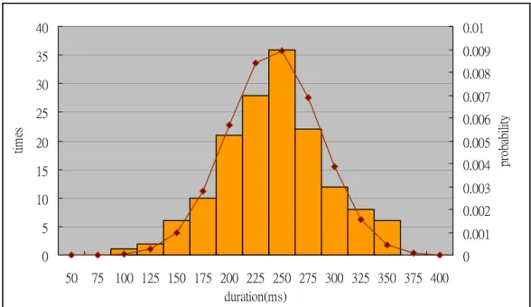
According to previous work [2][7][9][16], the duration distribution of each digraph forms an approximate Gaussian distribution. Therefore, we make the assumption that n-graph g with duration d, which forms a Gaussian distribution, such that 2 2 2 ) ( 2 1 ] , | Pr[ g g d g g g e d σ μ

σ

π

σ

μ

− − = , (3.1)

where μ_g is the mean value of the durations for n-graph g, and σ_g is the standard deviation. If we collect numbers of the keying behavior of user during a while and count the appeared times for each duration, we can draw a statistical chart like Figure 3.1.

0 5 10 15 20 25 30 35 40 50 75 100 125 150 175 200 225 250 275 300 325 350 375 400 duration(ms) tim es 0 0.001 0.002 0.003 0.004 0.005 0.006 0.007 0.008 0.009 0.01 pr oba bi lit y

Figure 3.1: The distribution of digraph duration

Hence we utilize the probability density function of Gaussian Model to calculate the behavior probability of user. Gaussian Model indicates that the n-graph durations of test samples closer to the mean of n-graph durations of reference samples occurs at higher probability. Likewise, the n-graph durations away from the mean occurs at lower probability.

In most work, the mean and standard deviation are usually decided by the reference samples collected during the training phase (or registration phase), and the change of keying behavior is considered rarely. As time goes on, the accuracy would decrease since the user’s behavior might change. Some works [4][11][20] updated the reference data using the latest successful authentication entries to keep up with the variations of user’s behavior over time. In our model, the tendency of behavior change is seen as the other feature of user. Therefore, we want to estimate the appropriate mean and standard deviation according to the behavior change. In next section, we will introduce the Autoregressive Model from statistical prediction model.

3.3 Estimating Probable Parameters by Autoregressive (AR) Model

Since the mean and standard deviation affect the Gaussian distribution, we want to estimate the most probable value as the parameters of Gaussian Model. The statistical prediction model is used to estimate the possible value. The autoregressive (AR) model [28][29][31] is one of popular prediction model. It predicts next value of a system according to previous value. The AR model is often used with “moving average” (MA) as the ARMA (autoregressive moving average) model. Because the solution equations for the parameters of AR model are simpler and more developed than those for either MA or ARMA models [28][29][30], we choose the AR model to estimate the next possible value. Following the principle of AR model will be presented.

3.3.1 Definition of AR Model

Let a series { X } is said to be an autoregressive process of order p _t (abbreviated AR(p)) if t p t p t t t X X X Z X =φ1 −1+φ2 −2 +...+φ − + , (3.2)

where φ_i, i = 1,2,…,p, are the autoregression or predictor coefficient, and Z is white _t noise with zero mean and variance σ_z2. It means that the value of X at time t can be determined by the previous p values. We apply the AR model to estimate the next possible value because of this property.

3.3.2 Estimation of Coefficients

The predictor coefficients φ_i refer to how the previous values affect the expectation (next) value. There are a number of techniques for calculating the coefficients. The most two familiar methods are “Yule-Walker equation” [31] and “Burg algorithm” [31][32][33]. The former applies the covariance function to previous data,

and finds p equations which can solve the all φ_i. The later does not estimate the coefficients φ_i directly. It calculates the reflection coefficients (or part autocorrelations) by minimizing the forward and backward prediction errors. Burg’s algorithm is seen as the most reliable AR coefficients estimation method. It generates accurate coefficient estimates and makes the AR model stable [34].

Since the coefficients are determined by previous data, we need not to decide how many reference data should be included. Also, the coefficients express how reference data affect the model.

3.3.3 Order Selection

Generally, the AR model with higher-order will produce small estimated white noise variance. But the mean squared error, which depends not only on the white noise variance but also on errors form estimation of the parameters of the model, will be larger [31]. So, some criteria are proposed to assist with selecting suitable order, such as FPE, AIC, AICc, BIC, etc. According to their equation definitions, these criteria calculate some value with different orders. Then the order resulting minimum value will be the suitable order. However, it is inefficient using these criteria to select order in our model, since the parameters of different orders must be estimated. We just observe the results of some orders and make some suggestions.

3.3.4 Estimation of Next Possible Behavior

In order to estimate the proper values as the parameters of Gaussian distribution, the AR model is applied. Let dg(k), k = 1…m-1, denotes the duration of n-graph g for

each typing (totally m-1 times). For each n-graph g, we calculate the expectant duration

g

compute the difference between each dg(k) and μˆ as g x , that is, k

∑

− = − = 1 1 ) ( 1 1 ˆ m k g g d k m

μ

, (3.3) g g k d k x = ( )−

μ

ˆ . (3.4)

So, a series x = {x1,x2,...xm−1} will be generated. Then we utilize the Yule-Walker

equations or Burg’s algorithm to find the AR coefficients {φ₁,φ₂,...,φ_p}. Finally, ED _g can be calculated as follows:

∑

= − + = = p i i m i g g g d m x ED 1 ˆ ) (

μ

φ

. (3.5)

So, ED is taken as the mean _g μ_g of Gaussian distribution. And we calculate the root mean square (rmsg) as follows:

∑

= − = ′ p i i j i j x x 1 φ , p < j < m, p m x x rms m p j j j g _{− −} − ′ =

∑

− + = 1 ) ( 1 1 2 . (3.6)

The rmsg will replace σ_g when rmsg is smaller than sample standard deviation σˆ . _g

Otherwise, the sample standard deviation will be used to replace σ_g. Therefore, the new probability density function will be rewritten as follows:

2 2 ~ 2 ) ( ~ 2 1 ] ~ , | Pr[ g g ED d g g g e ED d σ σ π σ − − = , (3.7) } ˆ , min{ ~ g g g rms

σ

σ

= . (3.8)

3.4 Hidden Markov Model for Sequential Keystroke Analysis

Hidden Markov Model (HMM) [35][36][37] can be used to model sequential behavior, such as the sequence of keystroke timing information we intend to analysis in this paper. Generally, the Markov model is used to model a process that goes through a series of states [36], and has the property of Markov process. The states in the Markov model are observed directly. But in the Hidden Markov Model, the states are hidden and some outputs form the states are observed.

The basic HMM is shown in Figure 3.2. The shaded circles xi represent unknown

(hidden) states and the unshaded circles yi represent observed states, where i is a

specific point in time. The state transition matrix A contains the probability of transition from state to state. The state emission matrix η holds the output probability. The initial state probability π_i is the probability of starting at xi. A compact notation

} , , { η π

λ= A is used to indicate the complete parameter set of HMM.

Figure 3.2: The Hidden Markov Mode

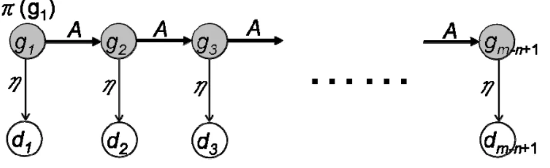
Now, we use the HMM to model the timing information of keystroke sequence. Given a keystroke sequence S, the set of n-graph G, and the set of [n+1]-graph G’, such that

{

}

} ,..., , , { ' } , , , , { , , , 3 2 1 1 3 2 1 2 1 n m n m N m m g g g g G g g g g G s s s S − + − ∈ ′ ′ ′ ′ = = = K K .

And we can illustrate the HMM for keystroke analysis of n-graph as Figure 3.3.

Figure 3.3: The HMMs for keystroke analysis

The n-graphs from the sequence are hidden state, while the durations of n-graphs represent the observed states. The state transition matrix A is compute as follows:

| | | | 1 i i g g g g A_{i i+} = ′ , (3.9)

where ||g′ and _i |g are the number of appearances in G’ and G respectively. The _i | state emission matrix η is defined as the Gaussian distribution probability, that is

2 2 ~ 2 ) ( ~ 2 1 ] ~ , | Pr[ ) ( gi i g i i i i i ED d g g g i i g d d ED e σ

σ

π

σ

η

− − = = , (3.10) where i g

ED is estimated by AR model and

i

g

σ~ is defined as (3.8). The initial

probability vector π is the probability of the frequency that the n-graph appeared in S, that is 1 | | ) ( + − = n m g g i i π . (3.11)

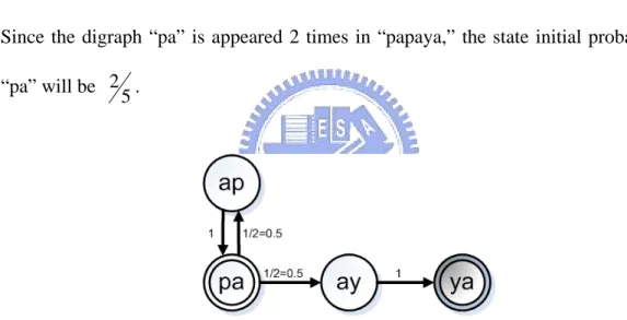
For instance in Figure 3.4, given a keystroke sequence “papaya” and digraph is interest.

Figure 3.4: Hidden Markov Model for keystroke sequence “papaya”

There are 5 (that is, 6-2+1) digraphs in “papaya.” For the digraph “pa,” there are two digraphs following the “pa” — “ap” and “ay.” (See Figure 3.5) As the result, the transition probability form “pa” to “ap” is 0.5

2

1 _{= , and so is that form “pa” to “ay.”}

Since the digraph “pa” is appeared 2 times in “papaya,” the state initial probability of “pa” will be

5 2 .

Figure 3.5: The graphical model for digraphs with sequence “papaya”

Each individual has his/her own HMM for the individual’s keystroke timing characteristics. Given a keystroke sequence and its timing information, the thing we should do is to calculate the behavior probability that the behavior belongs to someone’s. So, the modified Forward Algorithm is utilized to solve that problem.

Given a HMM with λ ={A,η,π}, keystroke sequence S with length m, the

{

}

} , , , , { } , , , , { , , , 1 3 2 1 1 3 2 1 2 1 + − + − ∈ = = = n m n m N m m d d d d GD g g g g G s s s S K K K .

Let α_t denotes the state probability of each state at time t. When t = 1, we can compute α₁ as follows: ) ( ) ( ) ( _{1 1 1} 1 g π g ηg1 d α = ⋅ . (3.12)

Then for each time step t=2,…,k, the stat probability is calculated recursively for each state. ) ( ) ( ) ( _{1 , 1} 1 + 1 1 + + t = t t ⋅ g g₊ ⋅ g₊ t t g α g A_{t t} η _t d α (3.13)

Finally, the behavior probability can be computed as follows:

[

]

( )

i g k i g g g k g g g k k k k d A d g d A g g GD G i i i k k k η η π η α α λ ⋅ ⋅ = ⋅ ⋅ = =

∏

= − − − − 2 1 1 , 1 1 1 1 1 ) ( ) ( ) ( ) ( ) ( | , Pr , (3.14) where k = m-n+1.

3.5 Authentication Scheme

There are three phases in our scheme for keystroke analysis: the training phase, the recognition phase, and the retraining phase. The training phase builds a database of user profiles during registration. The recognition phase compares test samples provided at login with the user profile in the database. If the user’s claimed identity is verified in recognition phase, the profile in the database will be updated in retraining phase.

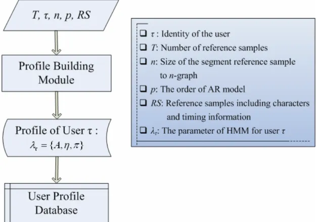
In the training phase, we will build the reference profile for each user. First, a number of reference samples of each target string are collected, and the size of n-graph to segment the target string as well as the order of AR model must be decided. After collecting a sufficient number of reference samples, we use the Autoregressive

Prediction Model to estimate the parameters of Gaussian Model for each n-graph. The transition probability matrix and initial probability vector with respect to Hidden Markov Model are also computed. The aforementioned data will be stored in the database as the reference profile of user. Figure 3.6 depicts the training phase process and the procedures of building profile are showed in Figure 3.7.

Profile Building Module :

Step 1: Transform the reference samples RS as n-graphs G and draw out the

durations of each n-graph as sample duration set SD.

} ,..., , {g₁ g₂ g_k G= )} ( ),..., 1 ( ),..., ( ),..., 1 ( ), ( ),..., 1 ( { 2 2 1 1 d T d d T d d T d SD k k g g g g g g =

Step 2: For each n-graph gi, apply the Autoregressive model with order p to

) ( ),..., 1

( d T

dg_i g_i and calculate the EDg_i and rmsg_i .

Let

σ

~g_i =min{rmsg_i,

σ

ˆg_i}.

Step 3: Compute parameters of HMM – the transition probability matrix A, initial

probability vector π, and emission probability matrix η.

)} ~ , ( ),..., ~ , ( ), ~ , {( 2 2 1 1 g g g gk gk g ED ED ED

σ

σ

σ

η

=

And let

λ

_τ ={A,

η

,

π

} denotes the HMM.

Figure 3.7: The procedures of Profile Building Module

In the recognition phase, the user claims an identity ID and provides a keystroke sequence TS as test sample. We wish to examine the possibility that the ID generated TS. First, we transform the keystroke sequence TS into n-graph combinations G and calculate the timing information of n-graph duration GD as usual. At this moment, we have

{

}

} , , , , { } , , , , { , , , 1 3 2 1 1 3 2 1 2 1 + − + − ∈ = = = n m n m N m m d d d d GD g g g g G s s s TS K K K .

Next, we retrieve the profile from the database based upon the claimed ID, including

ID

λ and parameters of each n-graph’s duration. Then the threshold vector GDT is

} ~ , , ~ , ~ { 1 1 2 2 1 1 − − −+ − −+ = n m n m g g g g g g ED ED ED GDT

ε

σ

ε

σ

_K

ε

σ

,

where ε is the weighting factor,

k

g

ED is ID’s expectation duration of n-graph g , _k

and

k

g

σ~ is the tolerated bias defined as (3.14). Then the Forward algorithm is applied

to GD, GDT, and λ , and two probability are obtained: behavior probability _ID ]

| ,

Pr[G GD λ and threshold probability _ID Pr[G,GDT |λ . _ID] Pr[G,GDT|λ is the _ID] possibility that all the n-graphs durations in G deviate ε times of duration σ~ from expectation duration ED , and used to decide that the acceptance of the keystroke sequence TS is confirmed if following expression is true.

] | , Pr[ ] | , Pr[G GD

λ

_ID ≥ G GDT

λ

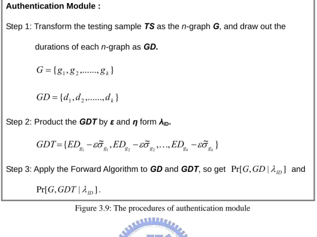
_ID (3.15)

The weighting factor ε can be specified with respect to different level of security strength. The recognition phase is showed in Figure 3.8 and the procedures of authentication module are showed in Figure 3.9.

Authentication Module :

Step 1: Transform the testing sample TS as the n-graph G, and draw out the

durations of each n-graph as GD.

} ,..., , {g₁ g₂ g_k G= } ,..., , {d₁ d₂ d_k GD=

Step 2: Product the GDT by ε and η form λID.

} ~ , , ~ , ~ { 2 2 1 1 g g g gk gk g ED ED ED GDT= −

ε

σ

−

ε

σ

_K −

ε

σ

Step 3: Apply the Forward Algorithm to GD and GDT, so get Pr[G,GD|λ_ID] and

] | ,

Pr[G GDT λ_ID .

Figure 3.9: The procedures of authentication module

If the testing sample passes the authentication, that is the expression (3.15) is true, that will enter to retraining phase. In the retraining phase, the passed testing sample is added to profile and recalculate the parameters. The procedures in this phase are like that in the training phase. Our model only used the latest numbers of sample data to estimate the expectation duration of each n-graph since the earlier sample data may be dissimilar to current behavior. Then the updating profile is saved back to database.

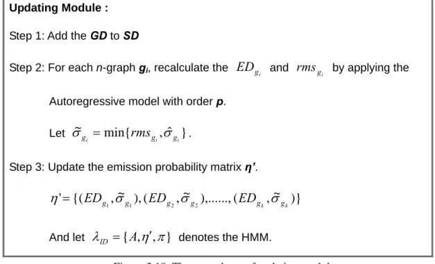
The retraining phase processes is showed in Figure 3.8 and the procedures of updating module are showed in Figure 3.10.

Updating Module :

Step 1: Add the GD to SD

Step 2: For each n-graph gi, recalculate the EDg_i and rmsg_i by applying the

Autoregressive model with order p.

Let ~ min{ , ˆ } i i i g g g rms

σ

σ

= .

Step 3: Update the emission probability matrix η’.

)} ~ , ( ),..., ~ , ( ), ~ , {( ' 2 2 1 1 g g g gk gk g ED ED ED

σ

σ

σ

η

=

And let

λ

_ID = A{ ,

η

′,

π

} denotes the HMM.

4. Experiments and Results

To evaluate our proposed model, we make an experiment to implement the described scheme in Section 3.5. In this chapter, the experiment will be presented. The settings of experiment and data collection are depicted in Section 4.1 and 4.2. Section 4.3 illustrates the ideal cases for the proposed model. Section 4.4 shows up the experimental results, and the discussion is in Section 4.5.

4.1 Experiment Settings

We conducted the experiment via web browser using a client-side JavaScript to gather the timing information of keystroke. Our sample population included volunteers from National Chiao Tung University as well as anonymous users form the Internet. Similar to a web-based application, the user inputted their username and password through as HTML form. In our experiment, we utilized a timing accuracy of one millisecond, and the segment size of keystroke sequence we analyzed includes the digraph and the trigraph.

We apply AR model with order 1~5 to calculate the parameters of Gaussian Model. The mean is estimated by AR model, and the mean square error (rms) is used to replace the sample standard deviation if the rms is smaller than sample standard deviation. The AR coefficients are estimated by Burg’s Algorithm. For comparison, we also analyze the user’s keying behavior without prediction. The non-predicting model uses the sample mean and sample standard deviation as the parameters of Gaussian Model. The EER1 (equal error rate) of authentication system will be obtained to compare.

1

Equal Error Rate (EER): the equal value of the error rate of false acceptance of imposter (False Accept Rate, FAR) and the error rate of false rejection of legal user (False Reject Rate, FAR).

4.2 Data Collection

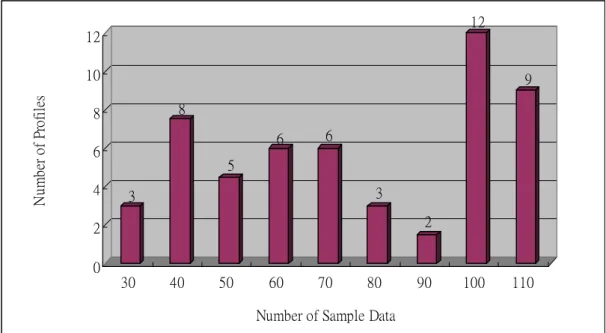
To generate reference samples, 53 volunteers supplied at least 35 samples of two strings (username and password) during 2 months. Figure 4.1 depicts the distribution of number of sample data. For each user, the first 20 sample data are used to train the model, and other sample data are used to authenticate their own account. The passed sample data are added to profile and the model will be retrained. Another 103 anonymous volunteers tried authenticate the accounts of legitimate users. Each account was attacked between 50 and 200 times for a total of 3126 imposter test samples.

3 8 5 6 6 3 2 12 9 0 2 4 6 8 10 12 N u m b er o f Pr of ile s 30 40 50 60 70 80 90 100 110 Number of Sample Data

Figure 4.1: The distribution of number of sample data

4.3 Ideal Cases

The assumption of our work is that the keying behavior of user trends to some regularity. So, we first analyze two ideal cases which confirm to the assumption. The first case is the keying behavior of user keeping consistent. In this case, most works usually have good accuracy. The second case is the keying behavior of user changing with some regularity, such as being slower or faster. Most works did not analyze this

case. But in our work, since the behavior change is predictable, the performance of our model is well. The comparative results of predictive and non-predictive model are showed in Table 4.1. As can be seen form the table, the prediction model can almost identify users exactly even if the user’s typing behavior changes.

Table 4.1: The EER comparative results of predictive and non-predictive model

EER

Case 1:

User keep the typing behavior steady (no variate)

Case 2:

User’s keying behavior change with some regularity

Without Prediction 2.57% 15.00% AR(1) 0.80% 0.88% AR(2) 0.80% 0.00% AR(3) 0.80% 0.00% AR(4) 0.80% 0.69% AR(5) 0.40% 1.27%

For comparison, there are four cases of behavior change in Figure 4.2, and the analysis results are depicted in Table 4.2. The first case is that the keying behavior of user keeps steady while the mean and standard deviation of digraph’s duration are 320ms and 8ms respectively. The other three cases are that the user keying behavior becomes faster while the average variations are 8ms, 16ms, and 32ms respectively. The FRR (false reject rate) is used to comparison. According to the results, without prediction, the FRR performs well only when user’s keying behavior keep steady, but drastically increases as the variate becomes obvious. If the trend of behavior change is regular, the results with prediction perform well whatever the variation is.

50 100 150 200 250 300 350 1 8 15 22 29 36 43 50 57 64 71 78 85 92 99 login times du ra ti o n( m s) steady variate = 8 variate = 16 variate = 32

Figure 4.2: The four cases with different behavior change

Table 4.2: Analysis results of four cases with different behavior change

Without Prediction AR FRR 21~60 61~100 21~100 steady 2.50% 2.50% 2.50% variate = 8 57.50% 100.00% 0.00% variate = 16 62.50% 100.00% 0.00% variate = 32 70.00% 100.00% 0.00%

4.4 Results

The comparative results of EER in experiment are showed in Table 4.3. As can be seen form the table, the EER of the system with AR(1) could down to 2.19%.

Table 4.3: Comparative results of EER in experiment

Analysis with Digraph Analysis with Trigraph

AR(1) 2.19% 2.93%

AR(2) 2.37% 2.81%

AR(3) 2.37% 2.68%

AR(4) 2.49% 3.08%

AR(5) 2.64% 3.08%

Since not all the keying behavior of users could be predicted, the ratios of users having improved accuracy are displayed in Table 4.5. There are half users whose identified accuracy is enhanced by predicting the behavioral trend.

Table 4.4: The ratios of users having improved EER

Analysis with Digraph Analysis with Trigraph

AR(1) 41.18% 50.00% AR(2) 50.00% 55.88% AR(3) 44.12% 44.12% AR(4) 55.88% 52.94% AR(5) 52.94% 55.88% Average 48.82% 51.76%

The average promotion of EER for each order of AR model depicts in Table 4.5. Table 4.6 represents the maximum promotion of EER for each order of AR model.

Table 4.5: The average promotion of EER with different order of AR model in the experiment

Analysis with Digraph Analysis with Trigraph

AR(1) 6.21% 5.79% AR(2) 5.17% 5.69% AR(3) 5.84% 5.49% AR(4) 5.73% 6.76% AR(5) 4.27% 6.64% Average 5.44% 6.07%

Table 4.6: The maximum promotion of EER with different order of AR model in the experiment

Analysis with Digraph Analysis with Trigraph

AR(1) 14.12% 16.06%

AR(2) 15.00% 16.06%

AR(3) 15.00% 16.26%

AR(4) 14.31% 27.47%

AR(5) 23.34% 27.47%

As can be seen form Tables 4.3 to 4.5, the order of AR model is the higher, the number of users having improved EER and the promotion of EER are both the more. But the large order of AR model is not appropriate because the calculation of coefficients will increase the load of system. The suggested order of AR model is 3 ~ 5.

4.5 Discussion

The EER of our proposed scheme ranges form 2.19% to 3.08%, which is better than other works in literature to our knowledge (generally higher than 3%). And the best

case 2.19% EER is even better than our previous work (2.54%). Figure 4.3 graphs the performance of several systems in EER or AFR2

. Since some works made experiments with small number of users, Figure 4.3 only lists the works which made experiments with enough number of users. However, most of them did not consider the behavior change of user typing.

ERR/AFR

2.19

0.00 2.00 4.00 6.00 8.00 10.00 12.00 14.00

Joyce and Gupta Bleha et al Magalhaes et al Ru and Eloff Anagun and Cin Yu and Cho Araújo et al Jiang et al Our Scheme

(%)

Figure 4.3: Equal Error Rate (EER) or Average False Rate (AFR) for several approaches ( Green Bar: apply machine learning methods; Blue Bar: apply statistical classification methods)

As can be seen form the experimental results, only half users have enhanced accuracy and the promotional range is not very large. It is because we only collect the keystroke data during two months. If the duration of collecting data is the longer, there will be the more users having enhanced accuracy, and the promotional range will be more obvious.

In the experiment, we analyze the keystroke sequence with digraph or trigraph.

2

According to the experimental results, the accuracy of digraph is better than trigraph in some case. But it is not clear to induce the gains and losses between digraph and trigraph.

5. Conclusion

The biometric verification mechanisms usually assume that the biometric must be physical or regular. But the biometrics may change over time, especially for behavior biometrics. Some works considered this factor by updating the user profile. In our work, the tendency of behavior change is regarded as a feature of user. So, we applied the Autoregressive Model to estimate the next possible behavior. According to the experimental results, the EER could down to 2.19%, which is better than other works in literature to our knowledge (generally higher than 3%), and even better than our previous work (2.54%). Especially as users type with some trend or regularly, their identified accuracy could be enhanced by predicting their keying behavior.

As to future work, we will discover other prediction methods to replace or combine the proposed scheme. And the proposed scheme can be extend to free-text analysis for continuous authentication.

6. References

[1] R. Spillane, “Keyboard Apparatus for Personal Identification,” IBM Technical

Disclosure Bulletin, Vol. 17, No. 3346, 1975

[2] R. Gaines, W. Lisowski, S. Press, and N. Z. Shapiro, “Authentication by

Keystroke Timing: Some Preliminary Results,” Technical report, Rand Report, 1980.

[3] R. Joyce and G. Gupta, “Identity Authentication Based on Keystroke

Latencies,” Communications of the ACM, Vol. 33, No. 2, pp.168-176, 1990.

[4] S. Bleha, C. Slivinsky, and B. Hussien, “Computer-Access Security Systems

Using Keystroke Dynamics,” IEEE Transactions on Pattern Analysis and

Machine Intelligence, Vol. 12, No. 12, pp.1217-1222, Dec. 1990.

[5] D. T. Lin, “Computer-Access Authentication with Neural Network Based

Keystroke Identity Verification,” International Conference on Neural Networks, Vol. 1, pp.174-178, 1997.

[6] M.S. Obaidat and B. Sadoun, “Verification of Computer Users Using Keystroke

Dynamics,” IEEE Transactions on Systems, Man and Cybernetics, Part B, Vol. 27, Issue 2, pp.261-269, Apr. 1997.

[7] F. Monrose and A. Rubin, “Authentication via Keystroke Dynamics,” 4th ACM

Conference on Computer and Communications Security, pp. 48-56, Apr. 1997.

[8] W. G. de Ru and J. H. P. Eloff, “Enhanced Password Authentication through

Fuzzy Logic,” IEEE Expert: Intelligent Systems and Their Applications, Vol.12, No. 6, pp.38-45, Nov. 1997.

[9] D. Song, P. Venable, and A. Perrig, “User Recognition by Keystroke Latency

Pattern Analysis”, Apr. 1997.

System for Multiple Users,” 23rd International Conference on Computers and

Industrial Engineering, Vol. 35, Oct. 1998

[11] F. Monrose, M. K. Reiter, and S. Wetzel, “Password Hardening Based on

Keystroke Dynamics,” Proceedings of the 6th ACM Conference on Computer and

Communications Security, pp.73-82, Singapore, 1999.

[12] O. Coltell, J.M. Badfa, and G. Torres, “Biometric Identification System Based on

Keyboard Filtering,” IEEE 33rd Annual International Carnahan Conference on

Security Technology, pp.203-209, 1999.

[13] F. Monrose and A. D. Rubin, “Keystroke Dynamics as a Biometric for

Authentication,” Future Generation Computer System, Vol. 16, Issue 4, pp.351-359, Feb. 2000.

[14] S. Haidar, A. Abbas, and A. K. Zaidi, “A Multi-Technique Approach for User

Identification through Keystroke Dynamics,” Proceedings of the IEEE

International Conference on Systems, Man, and Cybernetics, Vol. 2, pp.

1336–1341, 2000.

[15] P. S. Dowland, H. Singh H, and S. M. Furnell, “A Preliminary Investigation of

User Authentication Using Continuous Keystroke Analysis,” Proceedings of the

IFIP 8th Annual Working Conference on Information Security Management & Small Systems Security, Las Vegas, 27-28 Sep. 2001.

[16] D. X. Song, D. Wagner, and X. Tian, “Timing Analysis of Keystrokes and

Timing Attacks on SSH”, 10th USENIX Security Symposium, pp.337-352, Aug. 2001.

[17] Enzhe Yu and Sungzoon Cho, “Keystroke Dynamics Identity Verification - Its

Problems and Practical Solutions,” Computers & Security, vol. 23, pp.428-440, 2004.

Identification,” IEEE Security & Privacy, Vol. 2, No.5, pp.40-47, Sep. 2004. [19] Yingpeng Sang, Hong Shen, and Pingzhi Fan, “Novel Impostors Detection in

Keystroke Dynamics by Support Vector Machine,” Parallel and Distributed

Computing: Applications and Technologies, Springer, pp.666-669, 2004.

[20] Lívia C. F. Araújo, Luiz H. R. Sucupira, Miguel G.. Lizárraga, Lee L. Ling, and João B. T. Yabu-uti, “User Authentication Through Typing Biometrics

Features,” IEEE Transaction on Singal Processing, Vol. 53, No. 2, pp.851-855, Feb. 2005.

[21] S. Hocquet, JY Ramel, and H. Cardot, “Fusion of Methods for Keystroke

Dynamic Authentication,” Fourth IEEE Workshop on Automatic Identification

Advanced Technologies (AutoID'05), pp.224-229, 2005.

[22] S. T. de Magalhaes, K. Revett, and Henrique M. D. Santos, “Password Secured

Sites – Stepping Forward with Keystroke Dynamics,” Proceedings of the

International Conference on Next Generation Web Services Practices (NWeSP’05),

IEEE Computer Society, Washington, DC, pp.293, Aug. 2005.

[23] K. Revett and A. Khan, “Enhancing Login Security Using Keystroke Hardening

and Keyboard Gridding”, Proceedings of the IADIS Virtual Multi Conference on

Computer Science and Information Systems, 2005.

[24] M Villani, C. Tappert, G. Ngo, J. Simone, H. St. Fort, and SH Cha, “Keystroke

Biometric Recognition Studies on Long-Text Input under Ideal and Application-Oriented Conditions,” Proceedings of Conference on Computer

Vision and Pattern Recognition Workshop (CVPRW’06), IEEE Computer Society,

Washington, DC, pp.39, Jun. 2006.

[25] Y. Wang, GY Du, and FX Sun, “A Model for User Authentication Based on

Manner of Keystroke and Principal Component Analysis,” International

Aug. 2006.

[26] D. Hosseinzadeh, S. Krishnan, and A. Khademi, “Keystroke Identification Based

on Gaussian Mixture Models,” IEEE International Conference on Acoustics, Speech and Signal Processing (ICASSP 2006), Vol.3, pp.1144-1147, 2006.

[27] CH Jiang, SP Shieh, and JC Liu, “Keystroke Statistical Learning Model for Web

Authentication,” Proceedings of the 2nd ACM Symposium on information,

Computer and Communications Security (ASIACCS '07), Singapore, pp. 359-361,

20-22 Mar. 2007.

[28] Richard Shiavi, “Introduction to Applied Statistical Signal Analysis,” Aksen

Associates Incorporated Publishers, p.235-248, 341-387, 1991.

[29] R. Fante, Signal Analysis and Estimation – An Introduction, John Wiley and Sons, New York, 1988.

[30] W.E. Eltahir, M.J.E. Salami, A.F. Ismail, and W.K. Lai, “Dynamic Keystroke

Analysis Using AR Model,” IEEE International Conference on Industrial

Technology, Vol.3, pp. 1555-1560, 8-10 Dec. 2004.

[31] Peter J. Brockwell and Richard A. Davis. Introduction to Time Series and Forecasting, second edition. Springer, New York, 2002.

[32] J. P. Burg, “Maximum Entropy Spectral Analysis,” Proceeding of the 37th

Annual International Society of Exploration Geophysics Meeting, Oklahoma, Oct.

1967.

[33] R. Bos, S. de Waele, and P. M. T. Broersen, “Autoregressive Spectral Estimation

by Application of the Burg Algorithm to Irregularly Sample Data,” IEEE

Transaction on Instrumentation and Measurement, Vol. 51, No. 6, Dec. 2002.

[34] M.J.L. de Hoon, T.H.J.J. van der Hagen, H. Schoonewelle, and H. van Dam “Why

Yule-Walker Should Not Be Used for Autoregressive Modeling,” Annals of

[35] M. I. Jordan. A Introduction to Probabilistic Graphical Models. In Preparation. [36] S. Russell and P. Borvig. Artificial Intelligence, a Modern Approach. Prentice Hall,

1995.

[37] L. R. Rabiner, “A Tutorial on Hidden Markov Modes and Selected Applications

in Speech Recognitions,” Proceedings of the IEEE, Vol. 77, No. 2, Feb. 1989. [38] A. Guven and I. Sogukpinar, “Understanding Users' Keystroke Patterns for

Computer Access Security,” Computers and Security, Elsevier, Vol. 22, No. 8, pp. 695-706, Dec. 2003.

[39] L. R. Rabiner and B. H. Juang, “An Introduction to HMMs,” IEEE ASSP

Magazine, Vol.3, Issue 1, pp.4-16, Jan. 1986.